

Introduction
Accurate modelling of the dynamics of the ice sheets is a first step in determining their future behaviour under conditions of a changing climate. Thermomechanical models of ice-sheet dynamics are, however, necessarily highly non-linear and the appropriate description of the ice rheology over the complete range of stresses, strain history, crystal fabric and temperature found in the polar ice sheets raises substantial difficulties (e.g. Alley, 1992). Despite these and other problems, considerable success has been achieved in reproducing the general form of the present-day ice sheets using a fully coupled thermo-mechanical ice-sheet model (e.g. Huybrechts, 1990). One way to investigate the treatment of ice dynamics is to see how well the model is able to reproduce the present-day velocity field. Considering a fixed geometry, it is possible to calculate the diagnostic velocity field, also termed the dynamic velocity (e.g. Budd and Jenssen, 1989), from the surface slope, the ice thickness and an expression for the flow law. Employing a thermomechanical model requires running the model through a full glacial–interglarial cycle so that the thermodynamical part of the model can equilibrate. This is necessary to remove the effect of temperature on the flow parameters from the analysis. Unfortunately, direct in-situ measurements of surface velocity to compare the model with are very sparse.
It is also possible to calculate the mean ice velocity using the principle of conservation of mass. This is often termed the balance velocity. It is a function of the accumulation pattern (and ablation if relevant), the ice thickness and the surface topography of the ice. The latter is necessary to find the flow direction. The calculated balance velocities give an estimate of present-day dynamics if the ice sheet is in equilibrium. Although the balance velocity is a depth-averaged value, differences between it and the dynamic velocity may give information on a deviation from steady state but more likely point to shortcomings in the way the ice flow is described in the model. Of particular importance are deficiencies in the flow law and the occurrence of basal sliding, for which no general theories are available. Balance-velocity calculations are very sensitive to the geometric input and therefore need the best data sets available.
Until recently, the only data sets describing the geometry of the Antarctic ice sheet and bed were from a single source — the Scott Polar Research Institute (SPRI) folio maps (Drewry, 1983). Ice thickness and surface elevation were derived, primarily, from radio-echo-sounding flight lines, supplemented by small amounts of seismic data. The folio bed- and surface-elevation maps were digitized in 1984 to produce a 20 km grid data set of each. For the sake of brevity, these data sets will be referred to as the Budd grids (Budd and others, 1984). Substantial errors (in excess of 200 m) have been found in the Budd grid of the surface elevation (Bamber, 1994a) due to a combination of errors in the original map and in the digitization process. Despite these errors, the data sets have been used extensively in modelling the Antarctic ice sheet (Budd and others, 1984; Radok and others, 1986; Huybrechts, 1990), due to an absence of any suitable alternatives.
In this paper, a new surface-elevation data set has been derived from ERS-1 radar-altimeter measurements and combined with an improved ice-thickness grid to derive the best possible bed topography for areas of grounded ice. The purpose of these new data is to provide improved boundary conditions for both numerical ice-sheet modelling and the derivation of balance velocities. The Antarctic Peninsula has not been included in the study, due to the complexity of the ice cover in this region.
Data Sources
Surface elevations
For this study, eight 35d repeat cycles of ERS-1 radar-altimeter wave-form data were available European Space Agency, 1992), comprising over 20 million height estimates over Antarctica. The altimeter on board ERS-1 can operate in two modes known as “ocean” and “ice”. The latter mode has a lower-range resolution (by a factor 4) but can, as a consequence, maintain “look” over a larger proportion of the ice sheet and, in particular, over the steeper marginal areas. The coverage provided by one 35 d repeat of “ice-mode” data (after filtering, discussed later) is shown in Figure 1. Comparison with an earlier study using only “ocean-mode” data (Bamber, 1994a) indicates the improved coverage, especially around Fimbulheimen, the Lambert Glacier drainage basin, the Antarctic Peninsula and the margins of Wilkes Land. However, for surface slopes greater than about 0.65° (the half-power beam width of the altimeter’s antenna), the height estimates from the altimeter become unreliable. This affects 10% of the continent, predominantly near the margins. For these areas, and for the region south of the orbital coverage of ERS-1 (81.5°), data from the Antarctic Digital Database have been used (British Antarctic Survey and others, 1993). Near the margins, much of the elevation data from this source was derived from stereo-photogrammetry and is, therefore, of relatively high accuracy (± 10 m). For the region south of 81.5°, the data source was the SPRI folio map (based on over-snow and airborne pressure-barometer data) and, consequently, of poorer quality (Bamber, 1994a).
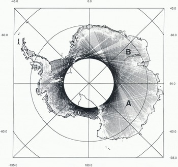
Fig. 1. The altimeter-data coverage after filtering, in ice mode, for a single 35 d repeat cycle of ERS-1. Also shown are the locations of the two ground-traverse data sets used. Set A is centred on Dome C and set B comprises two traverses running approximately along a contour line within the Lambert Glacier drainage basin.
Ice thicknesses
The most comprehensive compilation of radio-echo sounding (RES) data remains that which was used in the generation of the SPRI folio map series (Drewry, 1983). The coverage provided by this data set is shown in Figure 2. It is apparent that approximately half of the East Antarctic ice sheet contains no flight lines, In this area, there are only a handful of ground-traverse lines to provide ice thicknesses and the errors in values extrapolated from these lines are, inevitably, large. To provide the best possible data set for ice thicknesses, the RES data were used, where they were present. For the rest of the ice sheet, a redigilization of the SPRI folio ice-thickness contours was used. As a consequence, the accuracy in the gridded data set varies depending on the data source.

Fig. 2. Location of the radio-echo-sounding flight lines used in the compilation of the SPRI folio maps and the ice-thickness grid derived in this study.
The bed elevations were derived from the difference between ice thickness and surface elevation. This is only valid for grounded ice. At a later stage, to make the bed-elevation grid of more general use data for the sea floor beneath the ice shelves and on the continental shelf will be included. For the purposes of determining the velocity field, however, this was not required.
Altimetric Data Reduction
The processing of altimeter data over an ice sheet is complicated by the existence of topography with a significant surface slope. To improve the accuracy of elevation estimates over such surfaces, it is necessary to apply a range-estimate refinement procedure (known as wave-form retracking) and a slope correction to provide the correct range and location for the corresponding sub-satellite ground point. The former was carried out using the offset centre-of-gravity method of calculating the wave-form amplitude, with a power threshold of 25%. This threshold was chosen as it best represents the mean height over a topographic surface (Partington and others, 1989). Slope correction was applied using the relocation method with several modifications. These procedures have been described, in detail, elsewhere (Bamber, 1994b). As many repeat cycles as possible were used for a number of reasons: (i) it is possible to reduce some of the random errors by averaging the data, (ii) the cycles do not repeat exactly and there is about 1 km of across-track shift in the orbits, which helps provide the across-track slope required in the slope-correction procedure, and (iii) each cycle has a number of missing tracks, due to transmission or transcription problems with the raw data (as can be seen in Figure 1). By using several repeats, these missing tracks can be filled in, as they occur, in general, randomly (there are, however, a small number of tracks which are never obtained due to on-board recording limitations).
A number of problems have been associated with the wave-form data from ERS-1 which, in particular, affected the reliability of the internal range correction and the atmospheric corrections. We dealt with the former by applying a new correction based on a look-up table derived from the altimeter-engineering data. The latter we addressed from an analysis of 17 000 radiosonde profiles collected from 16 meteorological stations in Antarctica (Connolley and King, 1993). From these data, mean values for the wet and dry tropospheric corrections were derived. The resulting corrections obtained were

where △r d is the dry tropospheric correction and △r w is the wet.
Due to its relatively small size, the latter correction was ignored. The dry tropospheric correction was calculated using an adiabatic lapse rate of 9.7 × 10⁻³°Cm−1 to estimate the temperature change as a function of elevation. The total error in adopting these corrections is estimated to be ± 4 cm. The ionospheric correction was believed to be reliable and, like the wet tropospheric correction, is relatively small over Antarctica. The orbits used with the data were provided by the Technical University of Delft and have a global accuracy of ± 13 cm (Scharoo and others, 1994). The OSU91a geopotential model was used to convert from ellipsoidal heights to geoidal values (Rapp and others, 1991).
Considerable care was taken in the quality assessment of the data. The checks can broadly be separated into tests of wave-form shape, back-scatter coefficient and retracking-correction value. These tests were applied to remove data that were beginning to lose lock on the surface or had already done so before the instrument flags had declared loss of lock. Approximately 24% of the data were removed during this filtering procedure. A further step was required to remove the occasional spurious orbit. It was found that approximately one in 400 orbits was in error by several metres. This could only be detected by examining the eight repeats for each satellite track. Means and standard deviations (σ) were calculated for every point along the track and outliers were identified by the magnitude of the σ as a function of local surface slope. The σ threshold was determined from the pattern of crossing-point differences (described later).
Once the various corrections had been applied and filtering carried out, the data were interpolated on to a 10 km grid. A polar stereographic projection, with origin at the South Pole and standard parallel of 71°S was used to translate from polar to Cartesian coordinates. This is a standard projection used for Antarctica. However, it does not preserve area and, consequently, when calculating ice volumes and mean bed elevations, each grid-point value was corrected with the scale distortion for that point.
The spatial distribution of the altimeter data is highly anisotropic — height estimates are separated by 335 m along track and by 30 km across track at 60° S (Fig. 1). To prevent introducing biases on individual grid points (due to the spatial sampling pattern and grid spacing), a two-stage gridding procedure was employed. The first step involved splitting the data up into the boxes defined by the 10 km grid. Within each box, distance-weighted means of x, y and z were calculated, producing a quasi-regular array of average height estimates. A triangulation procedure was then used to interpolate to the exact grid-point locations (Renka and Cline, 1984). A similar methodology was employed for the gridding of the ice-thickness data. For the purposes of calculating total ice volume, thicknesses for the ice shelves were derived from the Digital Elevation Model (DEM) using equation (2) from Bamber and Bentley (1994).
South of the altimeter coverage, data from the Antarctic Digital Database were merged with the altimeter data by calculating the height offset at the boundary between the two data sets and using this to weight the Antarctic Digital Database data as a function of distance from the boundary. A distance-cubed weighting was found to provide a smooth transition and continuity of slope across the boundary.
The resultant 10 km DEM is displayed as a shaded planimetric relief map in Figure 3. The brightness is a function of both surface slope and elevation, decreasing with the former and increasing with the latter. This provides both the effect of perspective and contrast between features. Major ice divides appear bright, as do other flat, high-elevation areas such as the surface expression of the Vostok subglacial lake. The level of detail is also apparent; for example, the in-flow of Byrd Glacier into the Ross Ice Shelf and the Doake Ice Rumples on the Ronne Ice Shelf are both clearly resolved.

Fig. 3. A planimetric, shaded relief map of Antarctica derived from the 10 km digital elevation model.
Error Analysis
Random errors
The magnitude of the random errors in the altimeter data can be determined from an analysis of crossing points of descending and ascending tracks and from comparing repeat cycles for the same track. From such an analysis, the mean random error for a single data point was found to be ± 0.81 m (for a more comprehensive discussion of this topic see Bamber (1994a)). This value is an average over all the different surface types. The magnitude of the difference is correlated to surface slope due to the increased effects of topography on the accuracy of the retrack correction and nadir off-ranging effects (where the altimeter picks up returns from bright targets away from the nadir point). By averaging eight repeats, the random error is reduced to 0.29 m. However, not all the orbits were present for each repeat cycle and the mean number of repeats for a given track was nearer six.
The errors introduced by the non-uniform sampling and interpolation procedure were investigated using a simulated ice-sheet surface with sinusoidal undulations and similar track spacing to a 35 d repeat. The standard deviation of the difference between the grid point and the simulated surface was 5.05 m with a mean of zero. The relatively large error associated with the gridding procedure is due to the highly non-uniform distribution of data and the consequent undersampling of short wavelength topography in the across-track direction near the margins of the ice sheet. As with the cross-over distribution, the interpolation error is a function of location, decreasing inland due to the reduction in across-track spacing (Fig. 1) and “smoother” topography (McIntyre, 1986; Seko and others, 1993).
The standard deviation, for each grid point with sufficient data, was calculated dining the averaging procedure (the first step in the gridding process) and is displayed in Figure 4 as a shaded contour map. As with the cross-over distribution, the largest values lie near the margins and are closely related to the kilometre-scale surface roughness and ice thickness, which are, in turn, correlated with the surface slope. The plot, therefore, provides an indication of the height variability within each 10 km grid cell.
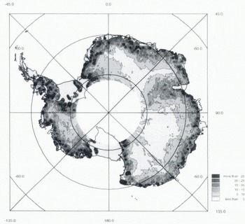
Fig. 4. Contour map of the standard deviation (in m) of the averaging procedure used in the first step in interpolating the radar-altimeter data on to a regular grid. The variance is closely related to the kilometre-scale surface roughness, which is, in turn, linked to the slope and ice thickness.
The total random-error budget on a single grid point, including the sampling error ranges from 10.7 m at 65° S and a slope of 0.65° to 1.4 m at 75° S and a slope of 0.1°. These errors are dominated by the height variability within each grid cell (Fig. 4) rather than errors in the individual altimetric elevation estimates.
Biases
Systematic errors in the altimeter data can be introduced from several sources including geographically correlated orbit errors (Scharoo and others, 1994), errors in the slope correction procedure and non-uniform spatial sampling.
To determine the absolute accuracy of the DEM, two ground-traverse data sets were used. The locations of these data sets are shown in Figure 1. Set A was obtained by GPS surveying techniques and has an estimated accuracy of ± 10 cm (Cefalo and others, 1994). The data are centred on Dome C, which is a relatively flat area where the altimeter would be expected to produce good results. Set B lies to the south and east of the Amery Ice Shelf and was collected during the austral summers of 1991–92 and 1992–93 (personal communication from M. Higham, 1993), These data come from a relatively sleep region with significant short-wavelength topography (as is evident from examination of the profiles–figure 5a (Bamber, 1994a)), where the data coverage is incomplete. The height estimates were obtained from GPS measurements every 30 km, with barometric elevations every 8–15 m in between. At control stations, the accuracy is 1 2 ms, rising to 5 m at the midpoint between controls (personal communication from M. Higham, 1993). DEM elevations at the traverse points were calculated using a bilinear interpolation procedure. Table 1 shows the mean difference (altimeter–ground traverse) and standard deviation for the two data sets.
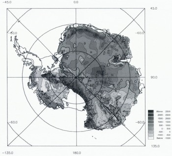
Fig. 5. Contour map of bed elevations derived from the new surface-elevation and ice-thickness grids obtained in this study. The contour interval used is 500 m. A coastline has been included in the diagram, to show the grounded-ice mask that was used. Note that the Antarctic Peninsula was not included in the present bed grid. The 0m contour is shown in bold.
Table 1. Statistics of the comparison between the two ground-traverse data sets and the altimeter digital elevation mode!

It is evident that the altimeter data over Dome C are accurate to well within the total error budget discussed in the last part of the section on random errors. For the Lambert Glacier data set, the high standard deviation is due, primarily, to short-wavelength (< 10 km) undulations that have been smoothed out in the altimetric DEM. Both data sets indicate that there is no significant bias in the altimeter data or the processing that has been applied to it.
Results
Surface elevations
The DEM derived from the combination of sources described earlier contains a number of improvements over the previously published data set obtained with ERS-1 (Bamber, 1994a). These include an improvement in the resolution of short-wavelength features, such as the ice streams draining into the Filchner–Ronne and Ross Ice Shelves. The use of the Antarctic Digital Database in the steepest 10% of the ice sheet has increased the reliability of the data in these regions. There is also, however, a general improvement in the altimetric coverage, and hence accuracy, in the marginal regions of the ice sheet below the angular cut-off of the radar antenna (approximately 0.65°). The precision of the height estimate has also improved with the use of the wave-form data due to (i) improved filtering, (ii) the capability to retrack the data and (iii) a greater number of repeat cycles and the improved coverage of the ice mode which, in turn, has improved the slope correction. The random error on a single point has been reduced from 4.8 to 0.81 m (based on a crossing-points analysis). Combined, these improvements have significantly reduced the error of the surface slopes derived from the DEM. Surface slope determines the magnitude of the gravitational driving force and provides the direction of flow. Estimation of balance velocity is highly sensitive to local errors in slope direction. The surface slope (over distances over which the driving stress is typically calculated) is now the best-known boundary condition available and the limiting variable on the accuracy of the balance-velocity calculation is currently the ice thickness and/or accumulation distribution, depending on the region.
Ice thickness
A visual comparison between the SPRI folio map and the gridded data set derived here shows no differences. This is reassuring, as the two maps were derived from the same original data source. However, a calculation of the total ice volume produces a value of 2.66 × 10⁷ km3 as opposed to the value of 3.01 × 10⁷ km3 estimated previously (Drewry and others, 1982) from the same data source and is closer to earlier estimates of ice volume (Thiel, 1962). The difference represents a discrepancy of 12% in the total volume of the ice sheet and ice shelves. This is significantly larger than the estimated error budget of 8% (Drewry and others, 1982). Similarly, the mean ice thickness calculated here is 2014 m compared, with 2160 m in Drewry and others (1982).
It is difficult to see how a bias could be introduced in the methodology adopted here for calculating ice thickness which involved summing the mean value for each complete cell (represented by the average of the four grid points of the cell) and correcting for the projection scale distortion. This is equivalent to one of the methods used previously (Drewry and others, 1982, equation (3)) but more rigorously applied and to a considerably finer grid. In particular, considerable attention was given to the interpolation procedure used. Several different methods were investigated which all gave the same result for ice volume and mean thickness and none of the methods used introduced a mean bias. The source for the substantial discrepancy between the present data and Drewry’s result therefore remains nuclear.
A crossing-points comparison of the RES tracks that we made produced a standard deviation of 198 m for 665 values. This is approximately 10% of the mean ice thickness, which is considerably worse than the 1.5% error estimate quoted by Drewry and others (1982). The discrepancy is most probably due to errors in digitization of the RES films and navigation errors. Where there are no RES flight lines, the errors in the ice-thickness grid will be significantly larger, although it is difficult to determine this precisely and no indication of this is given with the original data source. Visual examination of the data coverage in these areas and the magnitude of the ice-thickness gradients, where there were RES data, suggests that the errors could be in excess of 1000 m over distances of 200–300 km. Major deepenings such as the Bentley Subglacial Trench (in West Antarctica) or the Aurora Subglacial Basin could be completely undetected over a substantial part of the East Antarctic ice sheet.
Bed
The bed-elevation grid was derived from the difference between ice-thickness and surface elevation. Clearly, any errors in the ice-thickness grid will be reflected in the bed elevations. For this study, only the grounded ice is relevant and hence data below the ice shelves were not included. Furthermore, due to its complex terrain, the Antarctic Peninsula was not included in this study. The grounding line was estimated from the magnitude of the second derivative of the DEM (the rate of change of slope). Comparison of this estimate with data from other sources for the Ross Ice Shelf (Bamber and Bentley, 1994; Jacobel and others, 1994) suggests that this approach worked well, except for some of the ice streams in the eastern side of the Ross Ice Shelf. Here, a test for flotation was added, based on measurements derived elsewhere on the Ross Ice Shelf (Bamber and Bentley, 1994).
A shaded contour plot of the new bed topography is shown in Figure 5. With a contour interval of 500 m, differences between this data set and the SPRI folio map (Drewry, 1983) are not easily seen. However, it was possible to make a quantitative comparison between the bed elevations calculated here and the Budd grid. This is shown in Figure 6 as a difference plot (our grid minus Budd’s). It is apparent that there are substantial differences (> 600 m) between the two grids. Most of the differences are due to errors in the original (1984) digitization of the folio maps. These errors were also apparent in the surface-elevation data (Bamber, 1994a) and are folded into the Budd ice-thickness grid also as this was not digitized separately but derived from the surface-and bed-elevation grids.

Fig. 6. Map of the differences (in m) between the bed grid derived here and the one obtained in 1984 from the SPRI folio. A positive difference means that the bed in the Budd data set lies below ours. The 0m contour is shown in bold.
Ignoring the digitization errors in the Budd grid and comparing the SPRI folio with the new bed-elevations data set in detail indicates some subtle differences. In this case, differences are due entirely to errors in the folio surface-elevation map. The folio bed-elevation map has not been redigitized so it has not been possible to produce a quantitative estimate of the differences. However, a careful visual inspection indicates that there are significant differences in the region of Princess Elizabeth Land (70° S, 78° E), Dronning Maud Land–Coats Land (which is too high in the folio map), the Pole of Inaccessibility (81° S, 40° E) and in the vicinity of the Bentley Subglacial Trench.
A histogram of the distribution of bed elevations is shown in Figure 7. I is not possible to compare this directly with figure 4c from Drewry and others (1982) as it does not contain data from the ice shelves. It is, however, clear that the distribution of elevations is not Gaussian for this dataset: this result differs front that obtained by Drewry and others (1982). We found the mean bed elevation for the part of the ice sheet that is grounded to be + 142 m compared with − 160 m obtained by Drewry and others (1982) for the whole continent (including the continental shelf which is significantly below sea level). We also calculated statistics for the East Antarctic ice sheet only by including a mean bed elevation for the Amery Ice Shelf obtained from the folio map. We found a mean bed elevation of +251 m compared with + l5 m obtained by Drewry and others (1982). However, the precise region defined by Drewry and others as “East Antarctica” is not clear so even this comparison remains equivocal.
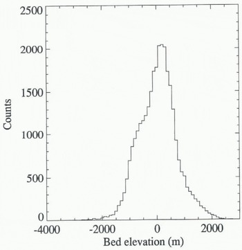
Fig. 7. Histogram of bed elevations for all areas included in the bed grid. Data were grouped into 100 m bins.
Discussion
The large differences between the Budd grid and the data derived here are likely to have a significant effect on the behaviour of the ice-sheet numerical model. Vertically averaged dynamic velocities depend on surface gradient to the third power and on ice thickness to the fourth power. A difference of ice thickness of 10% will thus lead to a difference in the modelled velocity of 46%. Additionally, ice thickness has a strong control on the basal temperature because of the insulating effect of the ice and this will in turn affect the flow-law parameter. The data derived here represent an improvement over the Budd grid in that they have been derived directly from the measurements and not as the difference of inaccurate digitizations of surface- and bed-elevations data. Nevertheless, the thickness error retains a strong regional variation depending on the density of the RES flight tracks.
In addition, there is a considerable gain in accuracy due to the new surface data. For surface slopes of 0.5°, which gives a height difference of 350 m over the 40 km typically required to calculate the driving stress, a total error of 1.5 m would imply a difference in velocity of only 1.3%. The error in velocity for a typical central Antarctic slope of 10−3 (using the new DEM) is about 4%. These errors are significantly better, by a factor 5–10, than those obtained using the Budd grids or the DEM in Bamber (1994a).
The magnitude of the differences in bed elevation are a substantial fraction of the ice thickness in parts of East Antarctica. In particular, there is an area more than 600 m too low in the Budd data set in Queen Mary Land (68–72° S, 110° E), where the ice thickness is in the range 1500–3000 m. The Lambert Glacier drainage basin is another area where the error in bed elevation is on the order of 25% of the ice thickness. Furthermore, the pattern of differences does not consist of regional tilts and biases but is random, leading to significant errors in bed slopes everywhere. These errors do not directly affect estimates of the dynamic or balance velocities but become important in model runs which involve the calculation of the free surface. For instance, the depth of subglacial channels controls the magnitude of the ice outflow and this will affect the surface morphology further upstream. The elevation of the subglacial terrain is also an important boundary condition for experiments concentrating on grounding-line migration or on the behaviour of the Antarctic ice sheet in much warmer climates (Huybrechts, 1994).
The non-Gaussian distribution of bed elevations (Fig. 7) is also of importance, as a number of studies have been based on the assumption that the bed elevations have a normal distribution (Drewry and others, 1982). Closer examination of the histogram indicates that elevations above approximately 150 m conform to a Gaussian distribution while those below do not. A plot of the location of the bed above and below this threshold reveals that about 70% of the area below 150 m is covered by RES flight tracks. This suggests that the Gaussian distribution (obtained for the areas devoid of RES flight lines) is an artefact introduced by the poor spatial sampling in these areas.
Conclusions
A new level of accuracy has been obtained in producing surface slopes and elevations over the Antarctic ice sheet. These data have been combined with an improved ice-thickness data set to provide bed elevations over grounded regions of the ice sheet. These data sets will be used as inputs into modelling dynamic and balance velocities. The major uncertainty in the calculation of balance velocity will now come from inaccuracies in the ice-thickness and/or accumulation data rather than the surface slope.
In the process of generating the data sets, the total volume of ice was calculated and found to be 12% smaller than the previous estimate by Drewry and others (1982). The difference is equivalent to 8 m in global mean sea level and is more than the entire volume of the Greenland ice sheet.
Comparison of the ice-thickness and bed-elevation grids that had been previously obtained from the SPRI folio maps indicates differences in excess of 600 m. In some areas the differences represents 25–30% of the total ice thickness. We attribute these large differences primarily to errors in the original digitization of the folio and, to a lesser extent, to errors in the folio surface-elevation map. These large errors will have had a substantial influence on both the dynamic and balance velocities derived from the original data sets.
Acknowledgements
We thank S. Tsiobbel for redigitizing the ice-thickness contours from the folio map, the Scott Polar Research Institute for allowing access to the RES data and the British Antarctic Survey for providing the RES data. We are also grateful to E. Tabacco for making available the GPS data from Dome C and to M. Higham for the Lambert Glacier traverse data. During this research, J. L. B. was funded by a U. K. NERC Earth Observation Lectureship, and P. H. was on leave with the Belgian National Fund for Scientific Research (NFWO).


