1. Introduction

Ice-surface roughness is a parameter of importance for many glaciological studies. Surface roughness, a derivative of microtopography, provides the high-resolution information necessary to characterize morphological types of ice surfaces and complements satellite data in investigations of surface features across scale. In turn, ice-surface roughness is a prerequisite for the analysis of satellite data because the surface properties influence backscattering and reflection of the satellite signal.

An open problem in the study of glaciers and ice sheets from satellites concerns the influence of morphological features of a resolution higher than that of the satellite instrumentation. For example, advanced very high resolution radiometer (AVHRR) data have a pixel size of 1km, altimeter data have an along-track repeat of signals of about 600 m and a much larger footprint and synthetic-aperture radar (SAR) data have a pixel size of 12–30 m depending on correction. Aerial video data resolve submeter to meter objects, depending on altitude."Subscale"geophysical information is the information that is lost in any one technology because it is only detectable at a higher resolution. For instance, SAR data yield subscale information for radar-altimeter data, and video data yield subscale information for SAR data. Radar-altimeter data do not show individual crevasses, but a signal lost due to lack of reflectance in a crevasse has a geophysical reason and is different from instrument noise. Surface roughness and scattering contribute to the values recorded by the SAR instrument as well as the altimeter. Surface roughness can be considered derivative or secondary information, as it is not the data intended to be recorded, but it influences the actual data.

Jakobshavn Isbræ was the object of this study because it is the world’s fastest-moving ice stream. In any scenario of break-up of an ice sheet, fast ice streams constitute the instability points in the ice sheet considered as a dynamic system. This work is part of an effort to construct a segmentation of fast-moving ice areas and their slower-moving surroundings, using analytical methods from structural geology, quantitative morphology, geostatistics, neural networks and videography (Reference Herzfeld, Mayer, Higginson and MatassaHerzfeld and others, 1996a, b; Reference Herzfeld and MayerHerzfeld and Mayer, 1997; Reference HerzfeldHerzfeld, 1999; Reference Mayer and HerzfeldMayer and Herzfeld, 2000). Satellite data are a good source for low-resolution studies and video data and photography for intermediate-resolution studies.

There was no instrument to measure surface roughness at a scale of decimeters to tens or hundreds of meters, with centimeter accuracy. The glacier-roughness sensor (GRS) was designed and built to fill this gap. The geostatistical analysis presented in this paper is based on such high-resolution GRS data from the Jakobshavn Isbræ drainage basin. Survey areas were chosen large enough such that the SAR images also lent themselves to geostatistical analysis, thus permitting a comparison of surface features (see Reference Herzfeld, Stauber and StahlHerzfeld and others, 2000).

Surface roughness is defined as a derivative of microtopography; as such it is related to micromorphology as opposed to investigations of material properties of ice such as dielectric properties, density, water content, etc. Scattering inside firn has been studied for passive-microwave data (e.g. Reference ZwallyZwally, 1977; Reference Rotman, Fisher and StaelinRotman and others, 1982; Reference Rott, Sturm and MillerRott and others, 1993).

In meteorology, roughness is usually described by a single parameter, the roughness length z0. Geostatistical surface analysis captures the complexity of surface roughness by using a feature vector of several components. Our approach is based on using the experimental variogram in a more exhaustive way than necessary for kriging, by extracting a number of parameters related to morphological features rather than to spatial continuity. Objectives are: (1) quantitative characterization of surface properties; (2) automated classification of ice-surface morphology; and finally (3) segmentation of glaciers, ice streams or ice-sheet areas into morphological provinces. Objective (1) is achieved in this paper.

GRS data, variograms and surface-roughness analysis are ideal matches for morphological characterization, because none of them require or provide absolute elevation values. Morphology is described not by the absolute elevation values but by the change of elevation in space, which is the derivative of elevation (as a spatial function) and is the mathematical definition of surface roughness. The GRS does not measure surface elevation (microtopography), but registers local changes, relative elevation (surface-roughness values). The variogram is calculated from incremental values according to the intrinsic hypothesis of geostatistics (Reference Journel and HuijbregtsJournel and Huijbregts, 1978).

2. Instrumentation: The Glacier-Roughness Sensor

The GRS is designed to survey roughness or microtopography of snow and ice surfaces with decimeter spatial resolution and centimeter accuracy. It works mechanically with electronic registration. The instrument consists of a 2 m × 2 m sled frame supporting eight survey arms that are hinged on a main crossbar and touch the ground. As the sled is pulled over the ice, the survey arms move freely over the surface, their ends following the ups and downs of microtopography. Angular motion of each arm is registered digitally by a small processor at the hinge, then sent to the central processor and logged by a computer in the survey box atop the sled, with a frequency of 10 Hz. If the sled is pulled at 1 m s–1, this translates into 0.1 m along-track spacing of observations. Across-track spacing of observations is 0.2 m for four arms on each side of the sled, with a 0.42 m gap in the middle to accommodate the ski tracks (caused by pulling the sled). Pitch and roll of the sled itself, caused by larger-scale undulations of the terrain, are registered by two clinometers. In the current version, the sled is hauled by a skier. Pulling by a snowshoer is also possible, but with skis it is easier to maintain a constant speed and smooth pull, and the track is narrower. In the Greenland experiment, we were always able to maintain a velocity close to 1ms⁻¹.

The instrument is of modular construction such that no component exceeds 2 m in length, and all pieces, except for the survey box, fit in ski bags. It is easily assembled in the field. This facilitates transportation by helicopter and planes at moderate cost. The GRS was designed by U. G. Herzfeld and H. Mayer and engineered and built in 1997 by engineers and mechanics of the Technische Abteilung, University of Trier, Germany, under the direction of W. Feller.

3. Jakobshavn Isbræ Geography and Scale-Dependent Coverage by Roughness Data

Jakobshavn Isbræ was selected for several reasons. As the world’s fastest moving ice stream, it plays a key role in investigations of the Greenland ice sheet (Reference Pelto, Hughes and BrecherPelto and others, 1989; Reference Echelmeyer and HarrisonEchelmeyer and Harrison, 1990; Reference Echelmeyer, Clarke and HarrisonEchelmeyer and others, 1991,Reference Echelmeyer, Harrison, Clarke and Benson1992; Reference Iken, Echelmeyer, Harrison and FunkIken and others, 1993; Reference Funk, Echelmeyer and IkenFunk and others, 1994). It is an advantage to test a new instrument where observations using traditional geophysical methods have already been made. A further advantage, and likely a reason for the amount of scientific attention the glacier has received to date, is its accessibility (by Greenlandic standards). Ilulissat, Greenland’s third largest town, is located at the mouth of Jakobshavn Isfjord and is served by the official Greenlandic airline one to several times a day.

Jakobshavn Isbræ flows from the inland ice and accelerates to 7 km a⁻¹ (19 md⁻¹; Reference Echelmeyer, Clarke and HarrisonEchelmeyer and others, 1991) or 20.6 m d⁻¹ (7.519 km a–1 Reference Pelto, Hughes and BrecherPelto and others, 1989) at the calving front. Faster-moving ice can be traced for 80 km up the ice sheet along the longer, wavy southern branch ("South Ice Stream"), which joins the shorter "North Ice Stream" along a feature called "the zipper" because of the pattern of merging crevasses (Reference Echelmeyer, Clarke and HarrisonEchelmeyer and others, 1991). Surface velocity is about 1000 ma"¹ 50 km upstream of the calving front (Reference Iken, Echelmeyer, Harrison and FunkIken and others, 1993). Ice thickness at the calving front is about 800 m, judging by floating icebergs that have turned on their side. The ice stream follows a geological trough that continues into the Isfjord. The center-line depth of the bedrock trough is up to 2520 m, which places the bed about 1500 m below sea level (Reference Clarke and EchelmeyerClarke and Echelmeyer, 1996). A shoal located at the fjord’s mouth blocks passage of the large icebergs into Disko Bugt. Occasionally the pressure of icebergs exceeds a threshold and an outburst into the bay occurs, when the large icebergs have melted sufficiently to cross the shoal. Calving volume is approximately 25–28 km³ a⁻¹.

The fast-moving ice stream is distinguished by its heavily crevassed surface. A segmentation into a succession of provinces of characteristic crevasse patterns can be achieved based on video data and aerial photography (Reference Mayer and HerzfeldMayer and Herzfeld, 2000). Investigation of high-resolution surface structures in areas without heavy crevassing is facilitated by surveys with the GRS. In such areas, wind, snowfall, surficial melting and influence of the underlying regional strain field are the dominant morphogenetic features. With the goal of a complete coverage in data collection and classification of surface structures in mind, it should be noted that it is either possible to discern surface patterns in video data or to operate the GRS safely on the ground; there is actually an overlap in scale of surface features that may be investigated.

During expedition MIGROTOP 97 (May-June 1997) GRS surveys were carried out in the ablation area of Jakobshavn Isbræ drainage basin, south of South Ice Stream. Survey areas area 3, area 4, and area 5 are located in the vicinity of the ice camp (68°58.712’N, 49°30.280’W; 864 ma.s.L). The camp was set up just outside the heavily crevassed area, south of the marginal area of the South Ice Stream, as determined by reconnaissance and video-survey flights in 1996. A shallow crevassed ridge in the ice separates the camp from the heavily crevassed areas to the north, but thin crevasse lines continue under the ice in survey areas area 4 and area 5. The camp lies in a shallow depression between a ridge in the north and higher areas in the south.

At the low-resolution end of the scale range, European Remote-sensing Satellite (ERS-2) SAR data received contemporaneous to our ground surveys and obtained from the European Space Agency (ESA) are analyzed using geostatistical surface characterization (Reference Herzfeld, Stauber and StahlHerzfeld and others, 2000). The large-scale surface features mentioned in the geographical paragraph are discernable on SAR images. There is an overlap in scale between analyses based on video data and analyses based on SAR data. Surface-roughness data collected with the GRS are important for SAR data analysis.

4. Morphological Characteristics of GRS Survey Areas

The objective of this study was to survey prototypes of high-resolution ice-surface morphology (ice-surface classes) and to characterize them quantitatively In the ablation area of Jakobshavn Isbræ drainage basin, the following morphological types were encountered and investigated (Fig. 1):

1. (a) Area 3 (ABOVE ICE CAMP) is characterized by a morphology of shallow ridges and valleys with the following individual feature types: (1) ridges, spaced 5–10 m apart, height about 0.3–0.5 m, the ridge tops are icy and almost bare of new snow; (2) small sastrugi exist in the valleys between the ridges; (3) small sastrugi exist in flat areas; the direction of the sastrugi is different from the direction of the ridges; the sastrugi are about 0.2 m high in stripe I and 0.4 m high in stripe G. The ridges are formed by meltwater (valleys are meltwater channels) and the sastrugi are formed by wind; (4) blue-ice patches. Area 3 is 175 m × 100 m, the along-track direction is 67°45’, the across-track direction is 157°45’.

2. (b) Area 4 (RIDGES) has a morphology similar to area 3, but the ridges are more pronounced, higher and more regularly spaced. The entire area 4 consists of elongated near-parallel ridges, partly gently wavy, with lows in between. These are clearly generated by melting (melting channels - valleys, ridges in between), not by wind. The height of the ridges increases in the uphill direction from area 3 to area 4 and throughout area 4 to more than lm in height in the upper part of area 4; their flanks steepened to more than 45° in area4n and area 4m. In area 4 ridge height falls into three classes: area4r; areas 4q, 4p, 4n; and area 4m. Area 4 is 175 m × 125 m and parallel to area 3.

3. (c) Area 5 (BLUE-ICE AREA) is 150 m × 50 m, parallel to area 3, and located at the southern foot of the shallow ridge mentioned above, in a blue-ice area. Water following a ridge-and-valley pattern down from the shallow ridge induces a pattern in the blue-ice area, creating an alternation of mostly frozen and daily melting/refreezing patches. The melting/refreezing ponds are about 5 m wide and 25 m long (20–50 m long) and trend 157°45’; shorter ponds are deeper than longer ones. The direction of these drainage features is oblique, at a small angle to the direction of the crevasses on the shallow ridge.

Fig. 1. Location and survey grids of area 3, area 4 and area 5. The grid is labelled using letters across-track and numbers along-track (K1…K8; J1…J8) (see Fig 4). Letters name 25 m stripes (e.g. area 3k); area 3k is between marker lines K1…K8 and Jl…J8; etc. Area3 is marked K, J, I, H, G, and 1…8, with stripes area 3k to area 3h. Area 4 is marked R,Q,P,N,M,L,andl..8, with stripes area 4r to area 4m. Repeat surveys of area 4p are named area 4pl, area 4P2, and area 4P3 Rl is about 100 m from Gl. Area 5 is marked V, U, T and 1…7, with stripes area 5v and area 5u. Inside each stripe tracks are labelled 1…10(or 1…11 or 1…9).

A survey to test the new instrument and collect reference data from a flat surface was undertaken on 20 May 1997 on lake Vandsø No. 4, located south of Mt. Akinaq and a few kilometers from Ilulissat airport (69° 13.56’N, 51°02.40’W; camp location). Data from areal, a snow-filled valley, are not reported here. Area 2, on frozen Vandsø No. 4, is 175 m × 75 m, the tracks run 52° E (long 175 m side). This dataset from the frozen lake surface with little old snow in places and little surficial melting locally towards the end of the survey provides a reference dataset, because the records show few structures, thus ensuring that records from flat areas do not contain any artefacts (see section 5).

5. GRS Survey and Data Processing

GRS surveys were carried out in survey grids which were established prior to the surveys (Fig. 1). Each survey area had to be: (a) large enough to contain sufficiently many repetitions of its characteristic morphological features; (b) small enough to be morphologically homogeneous; (c) large enough to encompass several SAR data pixels which might show some variability; and (d) small enough to be covered by a man-hauled instrument in a reasonable time. Areas 175 m long (along-track direction) and 75 m wide (across-track direction) were deemed optimal with respect to these four criteria.

Grids of 25 m were staked out using classical surveying methods and 12.5 m intermediate points marked along-track. The network was then surveyed using global positioning system (GPS) receivers. The main part of the survey is the GRS data collection. Surveying approximately normal to the general strike of the dominant morphological structures reduced the width of the area and thus saved on total survey time. Correlation lengths and spatial frequencies can then be determined easily from variograms of track data. Spatial covariation is higher in all other directions, highest in the across-track direction. A 25 m × 175 m stripe typically requiring 10 tracks takes about 45 min to cover with the GRS.

The time of instrument pass at each 12.5 m marker was recorded manually. When combined with GPS network positions and GRS time data, these pass times allow for referencing the GRS data to location. Between pass points GRS data were interpolated linearly to correct for variations in towing speed. Offsets between stopwatch, computer clock and GPS clock were corrected. GRS data were checked for gaps in data logging, then merged with the time data to extract data recorded inside the survey area, separate tracks and relate data to position. Raw GRS values were converted to elevation, requiring calibration of the GRS instrument prior to the survey. Elevation profiles could then be plotted relative to time to check for continuity of the operation. Finally, locations of the individual along-track measurements were adjusted using the along-track location corrections, and elevation profiles vs along-track distance obtained (e.g. Fig. 2a). The morphological analysis using variography is based on the elevation data related to along-track distance (see section 7).

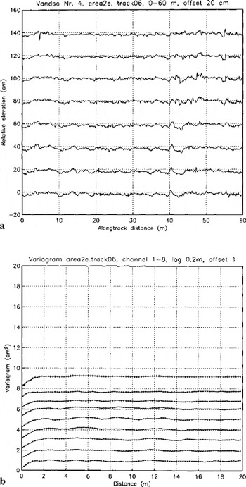
Fig. 2. Typical section of ice-surface roughness profile from GRS data and variogramsfor area 2, Vandsø Mo. 4, frozen-lake surface with little old snow frozen to lake ice. (a) Area 2e. track06, 0–60 m. Relative elevation corrected for along-track position. Data are offset by 0.2 per channel for easier display and only a 60 m section of each track is shown, (b) Variograms of roughness profiles of area 2 e.track06; offset by 1 cm2 for easier display (channel 1 at bottom, channel 8 at top). In this and the following two figures, variograms are calculated for entire tracks and plotted with the same scale on the vertical axis except for variograms of area4 xx indicates the variogram of an individual channel, channel 1 at bottom, channel 8 at top. +++ is the joint variogram of eight channels calculated in along-track direction with 90° tolerance.

6. Principles of Geostatistical Surface Characterization

The tool used to achieve a morphological characterization of ice-surface types is the variogram. The variogram is the spatial-structure function most commonly used in geostatistics. Originally applied as an aid in kriging (interpolation/ extrapolation of irregularly spaced data), the variogram is used here akin to the spectrum, but unlike the spectrum it is not as easily perturbated by errors over small distances, making it a more robust tool for the analysis of geophysical data than the spectrum. An advantage of the variogram over the (auto-) covariance function as well as over the spectrum is that existence of the covariance function and the spectrum require second-order stationary of the data, but the variogram exists under the weaker condition called "intrinsic hypothesis", which is second-order stationary of the increments calculated for fixed lags (with the increments considered a stochastic process):

Elevation is considered a regionalized variable z(x), defined throughout a two-dimensional region D and characterized by a structural aspect and a random variation (Reference MatheronMatheron, 1963). Then z(x) satisfies the intrinsic hypothesis if [z(x) - z(x+h)] is second-order stationary.

Herein lies the crucial point that makes variograms, GRS data, and surface-roughness analysis ideal matches for morphological characterization: Morphology is described not by the absolute elevation values but by the change of elevation in space, which is the derivative of elevation (as a spatial function) and that is the mathematical definition of surface roughness. The GRS does not measure surface elevation (microtopography), but registers focal changes and relative elevation (surface-roughness values). The variogram is calculated from incremental values, so the absolute elevation reference is not used nor needed. The task is now to use variograms to characterize, and classify, morphological types and we demonstrate how this is done in section 7. Under the intrinsic hypothesis, the variogram is calculated as

(1)

where z(xi), z(xi+h) are samples taken at locations xi, xi + h∊ D, respectively, and n is the number of pairs separated by ft. In our application, variograms with a lag of 0.2 m are calculated for each track (for the entire track, notjust for the sections shown in Figs 2a, 3a and 4a) in two ways, (1) for each channel separately, as a global variogram, and (2) for all 8 channels of one track together, as a directional variogram in the along-track direction with a tolerance angle of 90° (see Figs 2b, 3b, and 4b). The variogram for 8 channels combined is smoother, because more data are averaged, but generally has overall higher values because of larger differences to other channels.

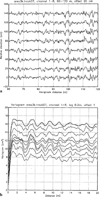
Fig. 3. Typical section of ice-surface roughness profile from GRS data and variograms for area 3 (ABOVE ICE CAMP), melting/refreezing ridges and channels with small sastrug in in flat areas, (a) Area 3 k.track07,60–120 m. Relative elevation corrected for along-track position. Data have been offset by 0.2 m per channel for easier display and only a 60 m section of each track is shown, (b) Variograms of roughness profiles of area 3k. track07; offset by 1 cm2 for easier display.

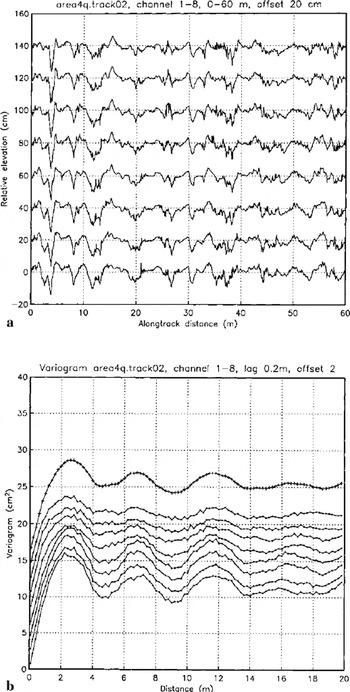
Fig. 4. Typical section of ice-surface roughness profile from GRS data and variogramsfor area 4 (RIDGES) larger melt-water ridges and valleys system with sastrugi superimposed. Dominance of ridges, (a) Area 4q. track02, 0–60 m. Relative elevation corrected for along-track position. Data have been offset by 0.2 m per channel for easier display and only a 60 m section of each track is shown, (b) Variograms of roughness profiles of area 4q. q.track02; offset by 2 cm2 for easier display.

If the variogram is used in kriging, a variogram model is fitted to match the transitive behaviour typical of a regionalized variable (low variogram values for short lags monotonously increasing to high variogram values for long lags). For lags exceeding a certain distance, the variogram "fluctuates" around a sill value, indicative of the total variance. These fluctuations are the source of information in geostatistical characterization and classification (Reference HerzfeldHerzfeld, 1999) which is applied here to study and describe ice-surface roughness. Roughness characteristics are captured in parameters that are extracted from the experimental variogram, these parameters constitute a feature vector. For characterization, feature vectors need to be selected that describe an ice-morphological type or ice-surface class uniquely. For classification, feature vectors also need to be selected such that each object encountered in a given area may be uniquely assigned to an ice-surface class from a given set of classes. Obviously it is necessary to first master the characterization problem before the surface-classification problem can be approached.

The following parameters are useful in characterizing the high-resolution surface structures from Jakobshavn Isbræ drainage basin (see Fig. 5): Maximum variogram value {fond parameter) is only the simplest parameter, it is used to distinguish flat areas from areas with morphological relief. The observation that the variogram of a wavy function is itself a wavy function leads to the mindist parameter, defined as the lag of the first minimum after the first maximum in the variogram. mindist gives the spacing of parallel ridges. The avgsPac parameter, defined as the average of lags to all minima in a variogram, also measures the spacing of dominant ridge structures.

Fig. 5. Schematic definition of geostatistical classification parameters: (a) pond parameter; (b) parameters p ₁ p₂ and mindist; (candd) in situations with subordinate structures superimposed on primary structures, parameter Vh is used instead of p2 and p₈ instead of Pl to obtain characteristic parameters of primary structures.

To distinguish pure hill-valley sequences from overprinted ones and to characterize more complex morphological structures, significance parameters are introduced:

(2)

(3)

p1 is the slope parameter and p2 the relative significance of the first minimum, mini, after the first maximum, max1, and h_× and γx denote lag and variogram value of x, respectively (Reference Herzfeld and HigginsonHerzfeld and Higginson, 1996). Parameters p3, p4, and p5 are used in addition to p2 to describe complex morphology.

(4)

(5)

(6)

Parameter p3 is the significance of the second minimum, mini, relative to the first maximum, p4 is the significance of the second minimum, mini, relative to the second maximum, max2, p5 is the significance of the second minimum, mini, relative to the highest previous maximum, maxs, where γmaxs is the maximum of γ max1 and 7max2. So if the first maximum is higher than the second, p5 = p3, otherwise it equals p4. Using p5 rather than p3 or p4 serves to better characterize morphologies with smaller features superimposed on larger ridge structures, as in area 3 ABOVE ICE CAMP. Similarly, slope parameters p6, pi, and p8 are defined; for instance p8 is the slope parameter analogous to p5:

(7)

Slope parameters involve the spacing. Relative significance parameters are independent of dimensions and thus facilitate comparison between different data sources, for example, surface roughness from SAR data maybe compared directly to surface roughness from GRS data using pi… p5.

7. Characterization of Ice-Surface Morphological Types Using Variography of Grs Data

In order to demonstrate and exemplify the principles of geostatistical surface characterization and classification theoretically introduced in the last section, profiles of GRS data from three morphological prototypes are presented and analyzed: (1) lake surface (area 2, Fig. 2); (2) complex surface with large ridges, ridge segments and small superimposed ridges (area 3, Fig. 3); and (3) simple morphology dominated by large ridges as observed in area 4 (Fig. 4). For reasons of brevity, data from area 5 are not presented. To indicate the range of variability in the geostatistical classification parameters of the GRS ice-surface data, parameters have been calculated for a number of profiles (Table 1).

Table 1. Geostatistical surface characterization parameters for selected profiles of GRS data from Greenland ice surfaces

Summary and Conclusions

The objective of geostatistical ice-surface characterization is to describe a morphological province or ice-surface class uniquely. Given appropriate data, this may be achieved using feature vectors of quantitative parameters extracted from experimental variograms, which are calculated from surface-roughness data.

The glacier-roughness sensor (GRS) is the first instrument designed and built to measure surface roughness or microtopography of snow and ice surfaces with decimeter spatial resolution and 10 mm accuracy in a continuous operation mode, while the instrument is pulled across the survey area. During the MICROTOP 97 expedition, the GRS was used to collect data from several 75 m × 175 m areas on the Greenland ice sheet. Location was established by GPS network data. Analysis of GRS data from areas representing different morphological types on Vandsø No. 4 (near Ilulissat) and on the inland ice south of Jakobshavn Isbræ South Ice Stream provided characteristic parameters to discriminate ridge-and- valley systems, lake surfaces, wind structures, melting structures and blue-ice areas. Variography, GRS data and surface-roughness investigation are ideal matches for morphological characterization of ice surfaces, because the variogram only requires existence and second-order stationarity of the increment process, the GRS collects relative rather than absolute microtopographic data, and surface roughness is the spatial derivative of the elevation function.

The parameters obtained in the characterization may be used further in a classification of the ice surfaces into high-resolution morphological types and, complementing a segmentation of the ice stream based on video data (Reference Mayer and HerzfeldMayer and Herzfeld, 2000), into a segmentation of the entire Jakobshavn Isbræ drainage basin. In a geostatistical analysis of ice-surface roughness across scales, SAR data and video data may be compared to GRS data and transfer functions established, such that it may be possible to classify larger areas using mostly remote-sensing data and GRS data only locally.

In addition to providing high-resolution morphological characteristics not otherwise attainable, GRS data may also yield ground truth for satellite-data analysis, where surface-roughness information is needed to understand the backscattering and reflection of the remote-sensing signal.