

Introduction
Fast-sliding ice streams and outlet glaciers have surface slopes related to the driving stress, and irregular topography with undulations reflecting the underlying bed topography. The undulations suggest the presence of localized “sticking points” on the bed, which may exert significant influence on the flow (Reference Whillans, Chen, van der Veen and HughesWhillans and others, 1989). In a recent inversion of high-resolution satellite-derived velocity measurements on a West Antarctic ice stream (Reference Bindschadler and ScambosBindschadler and Scambos, 1991), Reference MacAyealMacAyeal (1992) found that the distribution of basal friction derived from control theory is sensitive to the surface slopes. We therefore investigate the extent to which satellite radar altimetry can be utilized for high-resolution mapping of the topography of large ice streams and outlet glaciers, using Geosat ERM data from Lambert Glacier and upper Amery Ice Shelf (Fig. 1), which discharges an inland catchment area estimated at 870 000 km2 (Reference Giovinetto and BentleyGiovinetto and Bentley, 1985). This is about 9% of the area of the entire grounded East Antarctic ice sheet.
Lower Lambert Glacier, its grounding zone, and upper Amery Ice Shelf (Fig. 1) are within the Geosat coverage, and orbit convergence at 72.1°S resulted in a dense data set for this area, particularly for Lambert Glacier. The Geosat altimeter, although similar to the earlier Seasat (1978) version, incorporated design improvements that enabled it to maintain track more effectively over the Antarctic and Greenland ice sheets.
A contour map of ice elevations is constructed from Geosat ERM data by computing a digital terrain model (DTM), defined by a grid over the map area and an algorithm assigning a value to each grid node. The algorithm employed is kriging, an optimum estimation method based on the theory of regionalized variables (e.g. Journel and Huijbregts, 1978). (For an application to glaciology see Reference Herzfeld and HolmlundHerzfeld and Homlund, 1990.) Kriging is suitable for use with large data sets consisting of measurements arbitrarily distributed in two spatial dimensions, or distributed in a regular pattern such as along the repeat satellite ground tracks shown in Figure 2 (Reference Herzfeld, Hanley and MerriamHerzfeld, 1990). The noise levels in the data are estimated as a function of position throughout the map area using variogram methods (Reference Lingle, Brenner and ZwallyLingle and others, 1990). The standard error of the kriged map is estimated from the inferred noise levels in the data. A 3 km grid interval is chosen because that is roughly three times the ice thickness in the vicinity of the grounding line of Lambert Glacer. The horizontal resolution of the DTM should thus be sufficient for numerical models that take into account longitudinal stress gradients, while being coarse enough to warrant neglecting the “T term” (a double integral over a coordinate perpendicular to the glacier surface of the second derivative of the shear stress, in the longitudinal direction) in the longitudinal stress equilibrium equation (Reference Kamb and EchelmeyerKamb and Echelmeyer, 1986). An interpretation of the results is given.
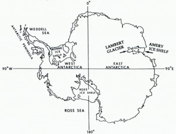
Fig. 1. Antarctica, with Lambert Glacier and Amery Ice Shelf indicated. The study area (box) is 70.5° –72.1° S, 67° – 73° E, or in UTM coordinates, 171 km north–south by 204 km east–west.
Data Processing and Spatial Distribution
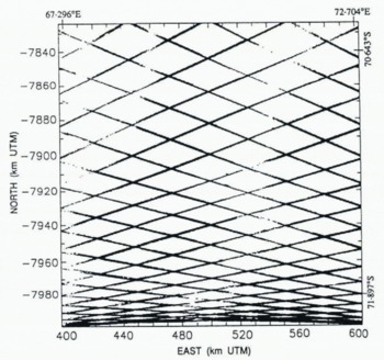
Fig. 2. Geosat ERM ground tracks in the Lambert Glacier study area.
Geosat ERM altimeter data from the Antarctic ice sheet have been reduced using Goddard Earth Model (GEM) T2 orbits (Reference MarshMarsh and others, 1989), and corrected for (i) tracking errors, using the method of Reference Martin, Zwally, Brenner and BindschadlerMartin and others (1983),(ii) atmospheric effects and solid Earth tides as described by Reference Zwally, Bindschadler, Brenner, Martin and ThomasZwally and others (1983), and (iii) slope-induced errors as described by Reference Brenner, Bindschadler, Thomas and ZwallyBrenner and others (1983), by the ice-sheet altimetry group at NASA Goddard Space Flight Center. The retracked Geosat ERM altimetry employed in this study extend from 9 November 1986 throughI 9 January 1989. This 792 d (2.17 year) period included 46 17 d orbit repeat cycles, and yielded 116 204 measurements of surface height throughout the map area. The GEM T2 orbits used in this preliminary study, which have a radial precision of about 0.35 m r.m.s. (Reference Haines, Born, Rosborough, Marsh and WilliamsonHaines and others, 1990), have not been adjusted into a common ocean surface. The altimeter-derived surface heights are with respect to the WGS 1984 ellipsoid.
The distribution of the along-track data is shown in Figure 2, which is a plot of all the individual measurement locations along the Geosat ERM ground tracks. The measurements are spaced at 662 m along the satellite tracks, for the 10 s−1 data used in ice-sheet altimetry. The ground tracks, which form a regular pattern because of the 17 d repeat cycle, are “fuzzy” because of the transverse orbit repeat variability of about 1 km. The diamond-shaped gaps are approximately 40 km east-west by 20 km north–south in the northern map area. The gaps become smaller in the southern map area due to convergence of the orbits at 72.1°S, at the southern map boundary. The continuity of coverage is very high relative to Seasat altimetry (compare to figure 2 of Reference Brooks, Williams, Ferrigno, Krabill, Oliver, James and JagoBrooks and others (1983), and to figure 4 of Reference Zwally, Stephenson, Bindschadler and ThomasZwally and others (1987)).
Map Projection
The map area, which extends from 70.5° to 72.1°S, 67° to 73°E, is 171 km north–south by 204 km east–west, when transformed to a rectangular area on a Universal Transverse Mercator (UTM) projection (Reference SnyderSnyder, 1987). Use of this projection results in (i) very low distortion, (ii) an orthogonal coordinate system, and (iii) distances that are defined in meters. Orthogonal coordinates are needed in kriging because the methodology includes a number of distance-dependent selection and interpolation algorithms. The datums are 0 m at the Equator for the north–south coordinate (northing with north positive), and 500 000 m at the central medidian, 70°E, for the east–west coordinate (easting with east positive).
Variography
The variogram is the spatial structure function — or spatial continuity function — used in geostatistics. Here, we empTloy variography in the estimation of a map showing altimetry noise levels and as a step in kriging. The ice elevation is considered a regionalized variable z(x), defined throughout a two-dimensional region D and characterized by a structural aspect and a random variation (Journel and Huijbregts, 1978). The variogram is calculated in bins according to:
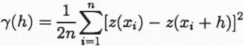
where z(xi), z(xi + h) are samples taken at locations xi, xi + hϵD respectively, and n is the number of pairs separated by the vector h. The spatial correlation among the elevations depends only on the vector h between the sample locations, a principle which the variogram shares with the structure function and the covariance function. The drift component m corresponding to elevation pairs separated by h is
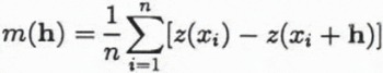
and the residual variogram is
Note that, if the regionalized variable z is stationary, then m(h) = 0 and γ(h) = res(h) for all h.
The experimental variograms calculated from the data are fitted by analytical variogram models to describe the transition from the strong covariation typical of closely neighboring samples to the weaker covariation typical of samples that are farther apart. The variogram model is characterized by its function type — which has to meet certain mathematical requirements so the inverse problem in the kriging step has a unique solution — and by parameters, which are the nugget effect C0, the sill C (where C0 and C are non-negative real numbers), and the range a (where a is a positive real number). The nugget effect or zero-lag intercept is the residual variance of resampling at the same location (see section on noise levels, below). The sill represents the a priori variance of the measurements. Elevation measurements separated by lags less than the range are spatially correlated. The range thus defines the maximum distance over which interpolation is meaningful. A linear variogram model with total sill C0 + C and range a is given by
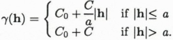
A Gaussian variogram, which is defined by
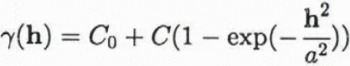
has a practical or quasi range of a′ = √3a with γ(a′) ≈ C0 + 0.95C (for a Gaussian distribution). The differentiability of the variogram at h = 0 is related to the smoothness of the regionalized variable. A linear variogram is associated with a regionalized variable that is continuous in a mean-square sense. A regionalized variable with a Gaussian variogram is mean-square differentiable. Use of a smoother variogram in the kriging estimation results in a smoother map.
Altimetry Noise Levels From Variograms
The noise levels in the data are estimated as a function of position throughout the map area using a method analogous to that described by Reference Lingle, Brenner and ZwallyLingle and others (1990). Briefly, the nearest 1000 height measurements (roughly the minimum needed to obtain “well-behaved” variograms) are identified within the circular neighborhood surrounding each node of a square grid with node spacing 10 km. These data are then used to compute an experimental residual variogram for the local neighborhood of each grid point, using Equation (3) (this differs from the method used by Reference Lingle, Brenner and ZwallyLingle and others (1990) for computation of residual variograms). The variogram for each grid point is extrapolated to zero lag (h = 0) using a polynomial least-squares fitting procedure, and the noise level is obtained as the square root of the zero-lag intercept, which is the standard error of the measurements in the local neighborhood of the grid point. Fourth-degree polynomials are employed, and are used only for extrapolating the variograms to zero lag. The polynomials thus need not (and do not) satisfy the mathematical constraints that analytical variogram models are subject to. The data noise estimates obtained in this way do not require a priori knowledge of instrument calibration, and represent the effects of all factors contributing to scatter in the data, including r.m.s. orbit error, systematic bias between ascending and descending orbits, noise caused by back-scatter from off-nadir undulations, and seasonal variations in penetration depth. Small-scale geophysical variations in the data cannot be discriminated from noise, however, and are thus incorporated in the “noise levels”. Crevasses are examples of such features.
The data noise levels throughout the map area, in meters, are shown in Figure 3, which indicates that the noise levels reflect the ice topography. The maximum noise levels (up to 150 + m) occur along the northwest boundary, where the American Geographical Society Map of Antarctica shows that the terrain is mountainous. The relatively low noise levels (3–10 m) in the north-central map area are characteristic of data back-scattered from the smooth surface of Amery Ice Shelf. The higher noise levels (10 m to about 50 m) in the south-central to southwest map area reflect the rougher and more undulating surface of grounded Lambert Glacier. The lower noise levels (10–20 m) along the eastern (right) map boundary reflect the relatively smooth surface of the high inland ice sheet. A “ridge” of higher noise levels coincides with the break-in-slope along the eastern margin of the glacier and ice shelf (see Figs 5 and 6).
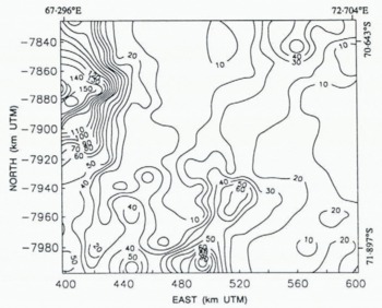
Fig. 3. Altimetry noise levels throughout the map area, computed using the variogram method (see text).
Geostatistical Computation of Digital Terrain Models (DTM)
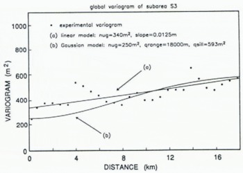
Fig. 4. Experimental variogram from sub-area S3 (marked on Figure 5) (discrete points), showing linear model (Equation (7)) used to krige DTM shown in Figure 5, and Gaussian model (Equation (5)) used to krige the DTM shown in Figures 6 and 7.
Kriging methods comprise a family of le ast-squares based on spatial estimation methods (Journel and Huijbregts, 1978). In this study, ordinary kriging, i.e. universal kriging of order 0, is employed for computation of the DTMs. The value Z0 = z(x0) at a node x0 is estimated using
where the Zi are altimeter-derived elevations Zi(x) at locations xi, i = 1,…, n, in the neighborhood of x0. The coefficients αi are determined such that the estimation error has minimum variance and the estimation is unbiased. The unbiasedness condition for ordinary kriging is α1 + α2 + … + αn = 1.
A solution is obtained using the variogram model derived from the experimental variograms. (For a derivation of the ordinary kriging system see Reference HerzfeldHerzfeld, 1992). The software used is specifically designed to evaluate data from geophysical line surveys (Reference Herzfeld, Hanley and MerriamHerzfeld, 1990).
Elevation data from a sub-area S3 on the surface of Lambert Glacier are selected for computation of directional variograms and residual variograms (Fig. 4), in order to use a spatial structure in the estimation that is appropriate for the area of main interest. To locate the grounding line it is necessary to detect a small change-in-slope on lower Lambert Glacier, so the spatial characteristics of the data from this sub-area are deemed most important. A consequence of using a single variogram for the entire DTM is that the rough areas along both sides of Lambert Glacier are somewhat smoothed. These areas, however, are not of primary interest in this study.
Variograms and residual variograms are similar for most lags, and can be fitted with the same model. The experimental directional variograms show effects that can be ascribed to the ground track pattern (i.e. jumps or wave-like patterns with approximately constant wavelength, superimposed on increasing variogram values). These patterns are disregarded in the model fitting. The linear model best describing the spatial structure in sub-area S3 is
(Fig. 4). The zero-lag intercept of 340 m2 (Equation (7)) implies a mean noise level of 18 m in the vicinity of the Lambert Glacier grounding line, which is roughly consistent with the independently computed data noise map shown in Figure 3.
The DTM is computed from the along-track data using variogram values from Equation (7). Each node of the 3 km grid is kriged using the nearest 16 altimeter-derived elevation measurements, selected with a quadrant seach algorithm (to avoid selecting only data distributed along a single ground track) controlled by a suite of parameters. The DTM has 68 grid nodes east–west by 57 grid nodes north–south. The corresponding map, with elevations in meters above the WGS 1984 ellipsoid, is shown in Figure 5.
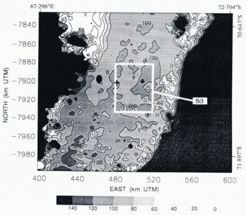
Fig. 5. Topography of lower Lambert Glacier and upper Amery Ice Shelf with DTM kriged using the linear variogram model (Fig. 4). The apparent grounding line of Lambert Glacier (100 m contour ) is accentuated in this gray-scale map. Elevations are in meters above the WGS 1984 ellipsoid. Location of sub-area S3 used for variogram calculation is indicated by the white box. The cross shows the location of the grounding line identified by Reference Budd, Corry and JackaBudd and others (1982) from optical leveling data.
To suppress somewhat further the effects of high noise levels in the data, a Gaussian variogram (see Figure 4 and Equation (5)) is used in a second run of the kriging procedure. The effect of a Gaussian variogram is that similar weights are assigned to the data closest to the grid nodes. The topographic effect is that the fine-scale roughness is smoothed. (Roughness on the scale of individual crevasses or “small” crevasse fields should not be resolvable in a DTM with 3 km grid interval, although Reference Partington, Cudlip, McIntyre and King–Hele.Partington and others (1987) showed that crevasse fields are detectable in the along-track, i.e. ungridded Seasat altimetry from Amery Ice Shelf). The Gaussian variogram model has a nugget effect of 250 m2 — corresponding to a mean noise level in the vicinity of the grounding line of 16 m, which is also roughly consistent with the data noise map in Figure 3 — a quasi sill of 593 m2 and a quasi range of 18 km. The variogram parameters are set such that at the quasi range, the quasi sill of the Gaussian model is equal to the 593 m2 sill of the linear model. The result is shown in Figure 6 as a map and in Figure 7 as a block diagram. The maps in Figures 5 and 6 are very similar. Areas of the same elevation on the glacier are somewhat more connected on the map based on the Gaussian variogram model (Fig. 6), however, than on the map based on the linear variogram model (Fig. 5). The major topographic features are the same, and in the same locations.
Error Analysis
The kriging estimation standard deviation (Reference Journel and HuijbregtsJournel and Huijbregts, 1989, p. 318) reflects simply the survey pattern. We therefore attempt to estimate the standard error of the kriged maps from the location-dependent data noise levels, using standard methods applicable to random error propagation through the kriging calculations. Taking this approach, it can be shown that
for the kriged elevation at node x0, where σ0 is the mean noise level for the data in the local neighborhood, and the αi are the optimum weights for the node (see Equation (6)). In this study, the αi were not saved along with the kriging output, but an approximate estimate of s0 can be made by assuming the weights are all identical, which is equivalent to supposing that each node is calculated as an unweighted average of the surrounding n height measurements. Using this approximation, s0 is simply σ0/√n, where n = 16 as noted above. (This simplification may yield a somewhat optimistic estimate of the map error, because the implication is that the error can be decreased substantially by increasing the number of points used to krige each grid node. In kriging, however, one reaches a point of diminishing returns, because points that are at greater distance have lesser weights.)
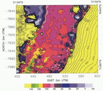
Fig. 6. Topography of lower Lambert Glacier and upper Amery Ice Shelf with DTM kriged using the Gaussian variogram model (Fig. 4). The apparent location of the grounding line of Lambert Glacier is the boundary between red (higher ) and purple (lower) meandering across the glacier approximately transverse to the flow direction. Elevations are in meters above the WGS 1984 ellipsoid.
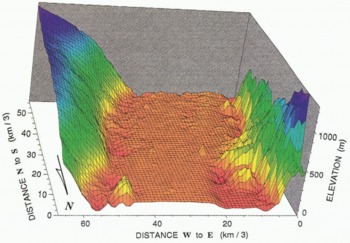
Fig. 7. Block diagram of upper Amery Ice Shelf (foreground) and lower Lambert Glacier ( background), kriged with the Gaussian variogram model. The vertical axis is meters above the WGS 1984 ellipsoid. The horizontal axes give numbers of grid nodes (grid shown on block diagram), 3 km per grid interval.
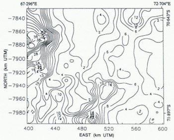
Fig. 8. Approximate Standard error of kriged elevation maps, in meters (see text section on error analysis).
Figure 8 shows the approximate standard error of the DTMs shown in Figures 5, 6 and 7; it is roughly one-fourth the data noise map shown in Figure 3, or 1–4 m on the flat Amery Ice Shelf, 4 m to about 14 m on the rougher Lambert Glacier, 2–4 m on the high East Antarctic ice sheet along the eastern map boundary, and up to 40 m in the region of mountainous nunataks along the northwest map boundary. There is also a “ridge” of higher map error — about 6–20 m — corresponding to the break-in-slope along the eastern margin of Lambert Glacier and Amery Ice Shelf.
It should be noted that Equation (8) does not include systematic errors caused by the inability of the altimeter to “see into” the dips between undulations. The back-scattered signals tend to be returned from the crests of undulations that are closest to the satellite, not from the nadir points, and the altimeter tends to “skip” from one high point to the next (Reference Gundestrup, Bindschadler and ZwallyGundestrup and others, 1986). The slope corrections partially account for this.
Interpretation
Glacier topography and location of grounding line
Most of the Amery Ice Shelf area mapped in this study is within the range 80–130 m above the WGS 1984 ellipsoid. It can be seen that the contours are more closely spaced and complex south of northing coordinates −7920 to −7930 km, suggesting grounded ice where basal undulations are transmitted to the surface through the fast-sliding ice stream. There are a number of spikes (perhaps 6) on the surface of the ice shelf and glacier in Figures 5–7, and these are caused by noise in the data. Beyond that, the irregular nature of the Lambert Glacier surface can be taken as a reflection of the more undulating and rougher surface characteristic of grounded ice.
The 100 m contour defines a break-in-slope suggestive of the grounding line. This break-in-slope can be seen in Figure 6, where it appears as the boundary between purple and red. This apparent grounding line meanders across Lambert Glacier in an irregular fashion. The patchy areas of red above the 100 m contour farther north suggest the presence of a number of sea-floor shoals intersecting the bottom surface of the ice shelf immediately downstream. The entire area, from northing coordinates −7870 to −7920 (on the western side of the glacier), or to −7950 (on the eastern side of the glacier), can probably be considered the grounding zone. The gray-scale map of Figure 5 shows the apparent grounding line (100 m contour) and sea-floor shoals more clearly. The grounding line identified by Reference Budd, Corry and JackaBudd and others (1982) from optical leveling data, shown by the cross in Figure 5, is within this grounding zone.
Reference Partington, Cudlip, McIntyre and King–Hele.Partington and others (1987) point out that the altimeter “sees” the grounding line before crossing it, when the direction of motion is up-glacier — or, conversely, after crossing it, when the direction of motion is down-glacier. An error of about 2–4 km is introduced, depending on the angle at which the ground track crosses the grounding line, if that effect is neglected. The data slope-correction procedure should counteract this effect, at least in part, but the “actual” grounding line may be displaced up-glacier on the order of 1 km to several kilometers from the apparent grounding line identified in Figures 5 and 6.
Ice-shelf and glacier margins
The block diagram in Figure 7 shows that Lambert Glacier and Amery Ice Shelf have lowered surface elevations corresponding to reduced ice thickness along the margins. These lowered surface elevations may be a consequence, at least in part, of enhanced vertical strain rates within the marginal shear zones. To show this, we adopt the conventional notation of ice mechanics. The stress tensor is σij, subscripts i, j represent directions x, y, z, where x is positive down-glacier, y is transverse, z is vertical (positive up), and x, y, z form a righthanded system, τij are shear stress components, τ is the effective stress, ⋵ij is the strain-rate tensor, B is the ice-hardness parameter, and n ≈ 3. The generalized flow law of ice is (Reference NyeNye, 1957):
where
is the second invarient of the stress-deviator tensor,
is the stress deviator tensor, and δij = 1 if i = j, δij = 0 if i ≠ j.
Consider a point “far” from the sides of Amery Ice Shelf. Vertical shear is negligible (Reference Sanderson and DoakeSanderson and Doake, 1979), and τxy is small because the transverse velocity gradient is small (Reference AllisonAllison, 1979; Reference Budd, Corry and JackaBudd and others, 1982), so
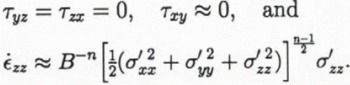
Within the zone of intense shear near the margins τxy ≠ 0, and is likely to be substantially larger than σ′xx, σ′yy and σ′zz so
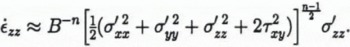
Thus, if the longitudinal stress deviator components are comparable in both places, the vertical strain rate ⋵zz (within the ice-shelf marginal shear zones) > ⋵zz (far from the marginal shear zones). If the grounded Lambert Glacier is moving mostly by basal sliding, the same argument would also apply, approximately, within its marginal shear zones. To account for anisotropy, Reference Jacka and BuddJacka and Budd (1989) found that the r.h.s. of Equation (9) should be multiplied by an “enhancement factor” E where for ice deforming in steady-state creep in compression with a preferred fabric, Eσ can be as large as ~3 (i.e. Eσ would multiply the r.h.s. of Equation (12)), while for ice undergoing steady-state shear deformation with a preferred fabric, Eτ can be as large as ~8 (i.e. Eτ would multiply the r.h.s. of Equation (13)). This suggests that the additional large shear-stress component τxy within the effective stress, combined with the effects of anisotropy, may be sufficient to account, at least in part, for the surface lowering along the sides of Lambert Glacier and Amery Ice Shelf. However, the optically levelled transverse elevation profile from upper Amery Ice Shelf in Reference Budd, Corry and JackaBudd and others (1982) shows that the elevations within the shear margins at the sides of the shelf are lower than the general surface by about 10–30 m. On the altimetry-derived maps in Figures 5–7, the elevations within the side shear margins are (apparently) lower than the general surface by about 50 m. Thus, “snagging”, an effect caused by the tendency of the altimeter to “lock on” to a reflector while crossing a break-in-slope before regaining track, may also account for a significant fraction of the surface lowering within the shear margins shown by the altimetry maps.
Summary
A geostatistical evaluation of the potential of satellite radar altimetry for high resolution mapping of Antarctic ice streams, carried out using Geosat ERM altimetry from lower Lambert Glacier and upper Amery Ice Shelf, East Antarctica, has shown that kriging can be used to obtain digital terrain models on a 3 km grid with an approximate standard error of about 4–14 m over the somewhat rugged surface of the grounded glacier and about 1–4 m over the flatter surface of the floating ice shelf (Fig. 8). The approximate standard errors of the DTMs are higher over the relatively steep slopes of the inland ice sheet immediately east of Amery Ice Shelf, and considerably higher (up to about 40+ m) over a mountainous region characterized by nunataks projecting through the ice sheet immediately west of Lambert Glacier and Amery Ice Shelf. These estimates of map error are based on the spatially varying noise levels in the data determined using variogram methods, and do not take into account systematic errors caused by not adjusting the orbits into a common ocean surface, or by the inability of the altimeter to “see into” dips between undulations occurring over short spatial scales.
The DTMs reveal undulations on the surface of the grounded Lambert Glacier that appear to be expressions of bed topography transmitted through the fast-sliding ice stream to the surface. The surface elevations are apparently lower within the shear margins along the sides of the glacier and ice shelf. This may, in part, be a consequence of enhanced vertical strain rates caused by the additional large shear stress component within the effective stress in the flow law of ice within the shear margins. This effect may also be, in part, an artifact of altimeter “snagging” (see “Interpretation” above).
A break-in-slope at about the 100 m elevation contour (above the WGS 1984 ellipsoid) is interpreted as the probable location of the grounding line. This break in slope, which meanders across Lambert Glacier in an irregular fashion, separates the higher and more rugged surface of the glacier from the lower, smoother surface of the ice shelf. Local areas of higher elevation on the ice shelf downstream from the apparent grounding line suggest the presence of sea-floor shoals projecting into the bottom surface of the ice shelf. The grounding line identified by Reference Budd, Corry and JackaBudd and others (1982) from optical leveling data along the central flow line is within the area generally identified as the grounding zone in this study. The “actual” grounding line may be displaced on the order of 1 km to several kilometers up-glacier (south) from the apparent grounding line in Figures 5 and 6, because of the effect of the slope change.
Acknowledgements
This work was supported by NASA grant NAGW-2614 and NASA/GSFC grant NAG 5-1748 to C. S. Lingle, and NASA grant NAGW-2746 to U.C. Herzfeld. U.C. Herzfeld wishes to thank the Alexander von Humboldt-Foundation, Bonn, Germany, for a Feodor-Lynen-Fellowship. We thank H.J. Zwally, A. C. Brenner, J. P. Dimarzio and S. Fletcher for furnishing the retracked and slope-corrected altimetry used in this study and for assistance with reading the tapes, R. Guritz for technical assistance with the Alaska SAR Facility IIAS computing system, O. Skulason and D. Covey for programming assistance, D. Sandwell for use of a color plotter, C. Rata for help with plotting and J. Griffith for production of the final figures. We also thank two anonymous reviewers and N. W. Young for comments that improved the manuscript.


