


1. Introduction
Sea ice is an important component of the Arctic climate system and its volume, areal extent and albedo are primary indicators of the state of climate in the central Arctic (Riihelä and others, Reference Riihelä, Manninen and Laine2013; Döscher and others, Reference Döscher, Vihma and Maksimovich2014; Landy and others, Reference Landy, Ehn and Barber2015). The Annual Mean Arctic sea-ice extent has experienced a pronounced decline with the rate in the range of 3.5–4.1% per decade (Pachauri and others, Reference Pachauri2014) along with significant reductions in annual mean sea-ice thickness from 3.59 m in 1975 to 1.25 m in 2012 (i.e. 65%) (Lindsay and Schweiger, Reference Lindsay and Schweiger2015), and ice age (Maslanik and others, Reference Maslanik, Stroeve, Fowler and Emery2011). These changes are accompanied by an overall increase in the sea-ice drift speeds (Kwok and others, Reference Kwok, Spreen and Pang2013; Kaur and others, Reference Kaur, Ehn and Barber2019). The ongoing Arctic sea-ice decline is not yet fully attributed to the underlying physical forcing mechanisms, but they include a temporally and spatially varying combination of dynamical processes, associated with changes in wind and ocean currents, and thermodynamic processes involving changes in air temperature, radiative and turbulent energy fluxes, and ocean heat storage (Francis and Hunter, Reference Francis and Hunter2007; Serreze and others, Reference Serreze, Holland and Stroeve2007; Deser and Teng, Reference Deser and Teng2008). Sea-ice drift speeds and patterns play important roles in the Arctic climate system and how the sea-ice drift patterns (Beaufort Gyre (BG), Transpolar Drift (TPD) and motion system in Kara Sea shown in Fig. 1a) have changed determines the advective part of the ice mass balance, i.e. the regional exchange of sea ice and export to lower-latitude oceans (Kwok and others, Reference Kwok, Spreen and Pang2013).

Fig. 1. Mean, std dev., skewness, kurtosis and per cent occupancy for sea-ice drift speeds from winter means of October 2006 to April 2018.
Gaussianity of geophysical data over time is the most common assumption in the earth sciences (Perron and Sura, Reference Perron and Sura2013). To determine whether a Probability Density Function (PDF) is Gaussian, higher-order statistical moments, such as skewness and kurtosis, are in particular used for the detection of outliers and of departures from normally distributed data (D'Agostino and Stephens, Reference D'Agostino, Stephens, D'Agostino and Stephens1986). These two moments (skewness and kurtosis) are explained quantitatively in the next section. The aim of this study is to provide a measure of whether higher-order statistical moments can be used to analyse the sea-ice drift patterns and how the non-gaussianity in the ice motion fields can be described in a concise and consistent way. This prompts the question of whether higher-order moments of variability contain further information about patterns in the sea-ice drift field, and how those moments might be interpreted. Our objectives are to (1) build diagnostics in order to understand the patterns of higher-order moments, (2) identify the spatial patterns of sea-ice drift using a new statistical approach, and (3) define an index for the BG and the TPD with higher-order moments. This paper is organized as follows: section 2 describes the data product and the processing of the data along with the techniques used for the analysis; section 3 describes the results and discussion; and is followed by the summary in section 4.
2. Data and methods
2.1 Data description
Previous studies demonstrated systematic error or bias in the NSIDC sea-ice drift product (Sumata and others, Reference Sumata2014), and more recent studies (Szanyi and others, Reference Szanyi, Lukovich, Barber and Haller2016) have demonstrated the existence of persistent artefacts associated with version 3 of NSIDC dataset and how those artefacts significantly impact the calculation of sea-ice motion gradients. Similar errors were also observed while performing the statistics of higher-order moments on the NSIDC dataset. In this study, we have therefore opted to use the low-resolution sea-ice drift product OSI-405-c from the European organization for the Exploitation of Meteorological Satellites (EUMETSAT) Ocean and Sea Ice Satellite Application Facility (OSISAF) (Lavergne and others, Reference Lavergne, Eastwood, Teffah, Schyberg and Breivik2010), despite its shorter duration of availability of the OSISAF OSI-405-c (2006 to the present) compared to the NSIDC ice drift product. However, the quality of the OSISAF ice drift product has been found to be superior to the NSIDC product based on comparison with the high random error (std dev.) and systematic error (bias) found in the NSIDC sea-ice drift product (Szanyi and others, Reference Szanyi, Lukovich, Barber and Haller2016). Low-resolution OSISAF ice drift datasets are computed on a daily basis from aggregated maps of passive microwave (e.g. SSMIS, AMSR2) or scatterometer (e.g. ASCAT) signals. They are all at the same spatial resolution, on the same grid and with a 48 h time span. Wide swaths, high repetition rates and independence with respect to the atmospheric perturbations permit daily coverage of most of the polar sea ice for fall, winter and spring. Ice drift vectors obtained from OSISAF have a spatial resolution of 62.5 km on a Polar Stereographic Grid. A distinctive feature of the product is that a sequence of remotely sensed images is processed by the Continuous Maximum Cross Correlation method, which builds on Maximum Cross Correlation method but relies on a continuous optimization step for computing the drift vector (Lavergne and others, Reference Lavergne, Eastwood, Teffah, Schyberg and Breivik2010). Only the data values in flag 30 (nominal quality) have been used for this work.
As the first step, we compiled all available drift speeds into a time series for winter defined as October through April. Sea-ice drift speed (magnitude of ice drift) is computed using the zonal and meridional components of ice drift, i.e.

where |U| denotes the speed, and u and v represent the zonal and meridional components, respectively, of the sea-ice drift computed from zonal and meridional displacements over a 48 h time span and frequency of OSISAF data.
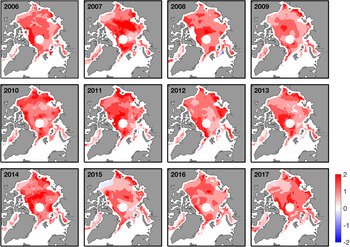
The results presented in Figure 1 were obtained by calculating yearly means (October to April) for the 2006–2018 period, and then determining the std dev., skewness and kurtosis for each pixel based on the 12 annual mean ice drift matrices with the size 119 × 177 pixels. Supplementary Figure S2 shows annual mean drift speeds and vectors for each year from 2006 to 2018. We further looked at each year individually by calculating the skewness and kurtosis based on daily ice drift datasets (Figs 2 and 3); that is, we used 212 matrices, of the size 119 × 177, where 212 (213 for leap year) represents the number of days in each winter from October to April. In all the figures in this manuscript, we have only plotted the values that are statistically significant as determined by the Bootstrap method. The bootstrap algorithm was used in order to obtain the standard error and margin of error for each pixel. The thresholds used were set according to the confidence interval of skewness and kurtosis obtained from the confidence interval using the difference/sum between the sample mean and the margin of error.

Fig. 2. Skewness for daily sea-ice drift speeds for 2006–2018.

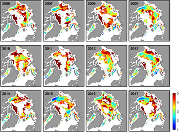
Fig. 3. Kurtosis for daily sea-ice drift speeds for 2006–2018.
2.2 Higher-order moments
Skewness and kurtosis, the third and fourth central statistical moments, were computed at each spatial gridpoint of the 119 × 177 ice drift matrices for the entire time domain in order to examine the spatial variability in the sea-ice drift field.
Skewness is defined as:

where μ is the mean of the relevant parameter x (i.e. either |U|, u or v), σ is the std dev. of x and N indicates the number of values (in this case daily (212/213) or annual (12) values for the October 2006 to April 2018 timeframe). The reference standard for skewness is zero, which represents the Gaussian distribution of the data. Skewness values less than zero (or alternatively greater than zero) are hereafter referred as negative skewness (or positive skewness) values. Skewness addresses the question of whether or not the ice drift speed is symmetrically distributed around its mean. Regional differences in skewness therefore show regional differences in sea-ice drift associated with rare large events that are reflected in the sign of the skewness.
Kurtosis describes the tails (peakedness) of the ice drift PDF. It is defined as:

The reference standard associated with Gaussian behaviour is 3 for kurtosis. In the context of an ice drift time series, a low kurtosis (i.e. K < 3) means that periods with either unusually low or high ice drift speeds are more rare compared to what would be expected from a Gaussian distribution, and the associated PDF tends to be flat near its peak and drops to small values faster than a Gaussian. However, when kurtosis is high (i.e. K > 3), extreme ice drift events occur more frequently and are more extreme compared to a Gaussian PDF. Hence kurtosis values less than 3 are referred as low kurtosis and kurtosis values higher than 3 are referred as high Kurtosis. Kurtosis provides a measure of intermittency and the frequency of extreme events. This moment can thus be useful to describe changes in the pattern of the sea-ice drift over long-term periods and in particular extreme events.
Luxford and Woollings (Reference Luxford and Woollings2012) used higher-order moments, namely skewness and kurtosis, to study atmospheric flow, and suggested that the patterns of skewness can arise as a kinematic consequence of the presence of jet streams. Hughes and others (Reference Hughes, Thompson and Wilson2010) suggest that kurtosis can provide a method of mapping mixing barriers in the ocean. We consider a similar approach here to identify patterns that distinguish circulation in the BG from transport associated with the TPD and changes in each as a function of space and time. In addition to drift speed |U|, zonal and meridional components (i.e., u, v) of ice drift are also evaluated to determine the relative contributions of each to spatiotemporal variability in the BG and TPD.
To account for seasonal variations associated with the presence and absence of sea ice, we compute per cent occupancy, defined as the ratio in the number of days during which the gridcell is ice-covered to the total number of days, for the timeframes considered (2006–2018, and annual). The percentage occupancy for each year on the basis of the daily dataset is shown in Supplementary Figure S1 and the mean percentage occupancy for 2008–2018 is shown in Figure 1e. The skewness and kurtosis patterns including those grid cells that fall within the 100% percentage occupancy contour indicate spatial structure depicted by the skewness and kurtosis associated with the winter ice cover, while patterns including those grid cells within the 80 and 60% occupancy contours indicate coherent structure associated with the sub-seasonal and marginal ice zone associated with the 2006–2018 and annual timeframes.
3. Results and discussion
Following the mean and std dev., skewness and kurtosis are the next two in series of moments, which characterize the shape of the PDF. The mean sea-ice drift field, based on 2006–2018 October–April (winter) average, indicates sea-ice circulation associated with the mean BG, TPD and Kara Sea ice circulation (Fig. 1a). The std dev. of the 12 winter mean ice drift speeds (Fig. 1b) indicates enhanced variability in the southern Beaufort Sea, and generally around the ice cover margins, associated with the poleward retreat in the sea-ice edge in these regions over the past decade. The spatiotemporal patterns for skewness and kurtosis (Figs 1c and d) indicate an underlying structure resulting in significant inter-annual variations in the mean drift speeds associated with extreme events and the frequency of these events in the sea-ice drift field. As previously noted, skewness is a measure of the asymmetry of the PDF. A PDF with a positive skewness has an enhanced right tail and the mass of the distribution is concentrated on the right of the figure and vice versa for negative skewness. Positive skewness values at a pixel indicate that a few years with the 2006–2018 period exhibited high yearly average ice drift speeds with large variation from the normal.
To evaluate the role of skewness in characterizing spatiotemporal variations in sea-ice drift features, consider the BG, where the gyre corresponds to the low drift speeds in the centre surrounded by higher drift speeds (Figs 1a and S2). When the centre of the gyre shifts its location, the occasional low drift speeds shift to the areas where usually high speeds are experienced and vice versa. Thus, this shift in the BG results in the positively skewed values in the centre of the gyre and the negatively skewed values in the surrounding areas. For BG, positive skewness indicates enhanced anticyclonic circulation, while negative skewness indicates cyclonic circulation (cf. Thompson and Demirov, Reference Thompson and Demirov2006). Thus, at a fixed point near the BG periphery, a shift to cyclonic circulation will reduce speeds in the direction of the flow, resulting in lower-than-normal ice drift speeds. By contrast, a shift to enhanced anticyclonic circulation will enhance speeds in the direction of motion leading to positive skewness. This will be further demonstrated in the evaluation of the zonal and meridional ice drift components.
From winters 2006–2007 to 2017–2018, statistically significant positive skewness values are found for the winter mean ice drift speeds along the periphery of the Beaufort Sea and in Kara Sea (Fig. 1c). In the Beaufort Sea, this pattern likely indicates occasional departures from low ice drift speeds associated with the centre of the BG (i.e. a shift or displacement in the BG from its mean). In Kara Sea, positive skewness indicates spatiotemporal variability/shifts in this sea-ice circulation regime. Negative skewness is observed in the TPD, in a manner consistent with negative skewness found at the core of jets in atmospheric flow fields (Luxford and others, Reference Luxford and Woollings2012), indicating the core of the TPD.
Kurtosis indicates persistent departures from Gaussian behaviour as well as persistent patterns in the mean winter sea-ice drift field from 2006 to 2018, and provides a signature of the frequency in extreme events. Kurtosis also indicates intermittency. High kurtosis values indicate that rare, large variation events occur more frequently than would be expected for a Gaussian distribution, thereby resulting in a more sharply peaked PDF with a broader tail than a Gaussian. By contrast low kurtosis values indicate that large or extreme events are rare.
From October 2006 to April 2018, statistically significant high kurtosis values in the Beaufort Sea periphery indicate extreme events evident in the tails of the sea-ice drift speed distribution, over space and time (Fig. 1), and characterize the spatiotemporal evolution in extreme events associated with the BG during the 2006–2018 timeframe. Specifically, statistically significant high kurtosis values are found in the periphery of the Beaufort Sea surrounded by comparatively low values, indicating frequent shifts in the centre and reversals of the BG (Fig. 1). Statistically significant high kurtosis is also observed in the vicinity of the TPD, indicating frequent high sea-ice drift speed features/events associated with the TPD during this timeframe. Percentage occupancy captures seasonal variations from 2006 to 2018 (Fig. 1e); 100% occupancy indicates the winter ice zone, while lower occupancy indicates the sub-seasonal ice zone. The central Arctic, Chukchi Sea and Barents Sea are characterized by 80–100, 60–80 and 0–40% occupancy ranges, respectively.
In Figure 1, we have shown that there is statistically significant interannual variability in the mean ice drift speeds across the Arctic Ocean. Here we will analyse in more detail how the higher-order moments vary within each 12 years of the OSISAF ice drift record from 2006 to 2018 (Fig. 2). The statistics for extreme events and the frequency of these extremes over each year is obtained by calculating the skewness over the daily ice drift speeds. The statistically significant positive skewness found throughout the Arctic Ocean for each year highlights temporal variability in large amplitude events (high drift speeds) between years. Slightly negative skewness of ~−0.2 in the Beaufort Sea is only found for winters 2015–2016 and 2017–2018 (Fig. 2). The negative skewness in the winter of 2015–2016 can be linked to the shift of the gyre towards the Chukchi Sea during December 2015, which resulted in the low drift speeds in the Beaufort Sea. Negative skewness is also observed in the Beaufort Sea region in 2017–2018, which may be attributed to an unusually thin ice cover and reversals in the BG ice drift in winter 2017 (i.e. February 2018) as ice drift speeds are reduced by flow opposite to the typical flow direction, as described in Moore and others (Reference Moore, Schweiger, Zhang and Steele2018).
Coherent and contiguous regions of high Kurtosis are observed in the central Arctic in the winters of 2006, 2008, 2010 (to a lesser extent) and 2016 in the winter ice zone (Fig. 3). These provide a signature of frequent large amplitude events characteristic of ice ridging, rafting, and/or opening and closing of leads and cracks in the ice cover. Low kurtosis is found in the sub-seasonal zone of the Beaufort Sea and Kara Sea, respectively, from 2006–2007, 2009 and 2015–2017. This provides a signature of rare large amplitude events and in 2017 in particular of BG reversals.
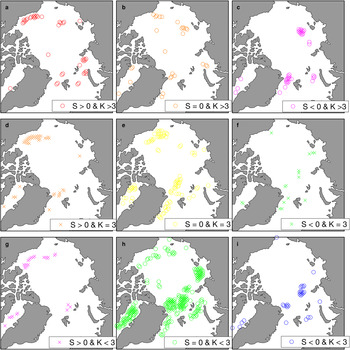
In order to characterize the BG and TPD and their spatiotemporal variability, an index is defined for combinations of high/low skewness and kurtosis regimes (Table 1 and Fig. 4). Statistically significant skewness and kurtosis in Figure 4 are computed using annual mean drift data and the bootstrapping algorithm, analogous to Figure 1. The skewness/kurtosis index further characterizes spatiotemporal variability in these patterns. Figure 4 highlights that a combination of skewness and kurtosis depicts spatiotemporal changes in the BG and TPD, with Gaussian values (S = 0, K = 3) capturing the core of the BG and TPD (Fig. 4e). Positive skewness characterizes extreme events associated with the BG, whereas negative skewness characterizes extreme events associated with the TPD. Kurtosis depicts the frequency of these events.

Fig. 4. Skewness and kurtosis combinations as shown in Table 1.
Table 1. Skewness/kurtosis index to characterize circulation patterns

Specifically, results show high skewness and kurtosis values in the southwestern periphery of the BG (Fig. 4a), indicating frequent large-amplitude (high drift speed) events associated with more mobile ice in a retreating and thinning ice cover in the Beaufort Sea region. Low skewness and high kurtosis values in the vicinity of the TPD indicate frequent low-amplitude (low drift speed) events north of the Siberian Islands and in Fram Strait (Fig. 4c), consistent with a recent study showing interruptions and reduced long-range transport in the TPD in a warming Arctic (Krumpen and others, Reference Krumpen2019). In summary, the Gaussian regime characterizes the BG and TPD, while negative skewness associated with low amplitude events (S < 0; K > 3, K < 3 – Figs 1c and d and 4c and i) indicates high-and low-frequency variations in the TPD, and positive skewness associated with high-amplitude events (S > 0; K > 3, K < 3 – Figs 4a and g) indicates high- and low-frequency variations in the BG.
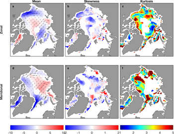
An evaluation of skewness and kurtosis in the zonal and meridional sea-ice drift components enables the identification of reversals (Fig. 5). The positive (negative) zonal component in Figure 5 shows the drift from west to east (east to west) and the positive (negative) meridional component shows the drift from the south to north (north to south), respectively. In Figure 5e, regions of positive/negative skewness in the TPD near Fram Strait and in the passage through the Franz Joseph Land and Novaya Zemlya can also be associated with the change in the course of the ice drift from Kara Sea. In some years, sea-ice drifting from the Kara Sea joins the TPD, whereas in others, sea-ice drifts via the Franz Joseph Land and Novaya Zemlya (Kaur and others, Reference Kaur, Ehn and Barber2019). In addition, positive skewness north of Fram Strait depicts meridional displacement in the TPD; when strong southward (negative) drift associated with the TPD is displaced eastward or westward into weaker (more positive) meridional drift regions, the TPD core experiences less negative meridional drift values, giving rise to positive skewness.

Fig. 5. Winter mean (a, d), skewness (b, e) and kurtosis (c, f) for the zonal and meridional component for 2006–2018.
Our analysis reveals negative skewness in the zonal ice drift component in the Beaufort Sea, and indicates the acceleration of the gyre. Drift in the meridional component also shows the negative skewness in BG, which further indicates acceleration in the gyre. Reversals are captured in less negative skewness values in zonal and meridional drift components in the western Beaufort Sea. In Figure 5f, K > 3 depicts more frequent normal meridional drift speeds in the BG gyre centre. Zonal sea-ice drift skewness is seen to range between −2 and 2 with negatively skewed values seen in the zonal component for BG and along the east Greenland coast. Negative skewness in the BG is the result of the enhanced westward advection in certain years, which result in values lower than the mean for that particular region. High meridional kurtosis also indicates zonal shifts in the centre of the BG. Positive skewness indicates that during some years, values higher than the mean for the respective areas are observed. Such variations in the BG can also occur due to the shift in the centre and reversals of the gyre.
Conclusions
In this study, we have examined patterns and spatiotemporal variability in sea-ice drift using higher-order moments to identify underlying structure in the sea-ice drift field, and spatiotemporal changes in the BG and TPD in particular. Departures from Gaussian behaviour in higher-order statistical moments provide a signature of spatiotemporal evolution in the BG and TPD and structure in the sea-ice drift field; an index is further derived based on the superposition of high/low skewness and kurtosis values that highlight regions where frequent and infrequent large-amplitude events occur. In this paper, the higher-order moments of skewness and kurtosis are used to characterize these non-Gaussian features. Our results suggest that the patterns of skewness arise due to the spatio-temporal shift in the drift patterns. Skewness is expected to accompany the shift in the centre of the gyre, while patterns of skewness and kurtosis can be used to identify changes in the circulation regimes within the Arctic. Our results show that skewness fields/patterns provide a signature of the BG and TPD over the 2006–2018 timeframe, and capture the spatial variability in the BG and TPD for this timeframe. High skewness (>3) indicates displacements in the BG periphery, while negative skewness captures variations in the TPD. Kurtosis provides a signature of frequency in extreme events. A skewness/kurtosis index derived through the combination of skewness and kurtosis regimes shows that the combination of positive skewness with high/low kurtosis provides a signature of central axis and the periphery of the BG, whereas negative skewness is found to characterize the TPD. Specifically, negative skewness associated with low amplitude events in the ice drift speed (S < 0; K > 3, K < 3) indicates high- and low-frequency variations in the TPD; positive skewness associated with high-amplitude events (S > 0; K > 3, K < 3) indicates high- and low-frequency variations in the BG.
The results obtained through this technique can further be used for model-data comparison, characterizing changes in dynamic flow field structure in a changing climate, as well as forecasting and prediction. In addition, the results obtained can also be compared to ice-ocean models to determine whether the model captures underlying structure in the sea-ice drift field, extreme events and the frequency of extreme events, which is of increased importance in an increasingly unpredictable Arctic (Lappäranta, Reference Lappäranta2011). Higher-order moments also enable a comparison with atmospheric and oceanic results to facilitate and improve our understanding of ice-ocean-atmosphere interactions from the perspective of dynamics. The significance of this study exists in the development of diagnostics and tools based on higher-order moments to determine whether models accurately capture increasingly unpredictable sea-ice conditions and more specifically sea-ice dynamics in the Arctic. The index map can in addition be used to identify regions with high/low frequency of high/low amplitude events, also relevant from the perspective of hazard and risk assessments, forecasting and prediction.
Supplementary material
The supplementary material for this article can be found at https://doi.org/10.1017/aog.2021.6
Acknowledgements
We thank the OSISAF for proving the sea-ice drift data. OSISAF data are available for academic purposes through the OSI SAF portal (ftp://osisaf.met.no/archive/). Thanks to the University of Manitoba Graduate Fellowship (UMGF) and Graduate Enhancement of Tri-Council Stipends (GETS). This is a contribution to the Arctic Science Partnership (ASP) and the ArcticNet Network of Centre's of Excellence. Thanks to the Scientific Editor Hester Jiskoot and three anonymous reviewers for their valuable time and constructive feedback.
Financial support
The funding for this work is provided through Canada Research Chairs funds to D.G.B. (grant number 301913).


 Open access