

Introduction
At the base of a polythermal glacier with a frozen margin, the transition from temperate-based ice to cold-based ice, herein called the basal thermal transition (BTT), is generally viewed as a slip/no-slip transition (Fig. 1). Although some glaciologists have documented basal motion at cold-based glaciers (e.g. Reference Echelmeyer and WangEchelmeyer and Wang, 1987; Reference Cuffey, Conway, Hallet, Gades and RaymondCuffey and others, 1999), it occurs at rates that are often more than an order of magnitude smaller than those of temperate glaciers. Therefore, rates of basal motion are expected to abruptly decline where fully sliding temperate-based ice transitions to fully coupled cold-based ice.

Fig. 1. Geometry and flow of a polythermal glacier terminus. Down-glacier from where the freezing isotherm dips into the bed, basal sliding is not permitted. This basal thermal transition (BTT) therefore represents a slip/no-slip transition.
Many authors have ascribed important processes to the BTT related to its role as a slip/no-slip transition. Among the most commonly cited of these processes is thrust faulting resulting from longitudinal compression (herein, a distinction is made between faulting, where there is slip along a discontinuity, and continuum flow where motion is accommodated by distributed strain without a discontinuity). This hypothesis seems to have arisen by analogy with crustal tectonics, and it finds support in some theoretical treatments of the problem. In models that represent flow of linear-viscous ice over a bottom boundary that has a discrete transition from free slip to no slip, a singularity in stresses and strain rates develops at the transition point. Beneath idealized glaciers this singularity, or the analogous case of a transition from no slip to free slip, has been the focus of several modeling efforts (Reference Hutter and OlunloyoHutter and Olunloyo, 1980, Reference Hutter and Olunloyo1981; Reference Barcilon and MacAyealBarcilon and MacAyeal, 1993; Reference LliboutryLliboutry, 2002), most of which employed analytical methods for obtaining asymptotic approximations around the singular point. Although each study attempted to extract a rigorous description of the ice dynamics in the area, each also acknowledged that the singularity was an unphysical result. Nevertheless, Reference Hutter and OlunloyoHutter and Olunloyo (1980) and Reference LliboutryLliboutry (2002) suggested that the high stress concentration at the BTT should cause erosion of the substrate or faulting within the ice.
Here we describe numerical experiments conducted to see how ice dynamics is influenced by a frozen margin with more realistic boundary conditions and ice rheology. For generality, we use two geometrically simple domains and treat the ice as a homogeneous medium. The intent is to relax some constraints, which have been motivated in part by mathematical convenience, to generate predictions of ice motion that can be more readily applied to glacier termini. Of particular interest is the treatment of conditions at the upper boundary of the glacier and resultant flow patterns as ice passes over the BTT. This modeling is also potentially relevant to transitions in basal coupling arising from factors other than temperature variations (e.g. soft-bed/hard-bed transition).
Background
Many modern polythermal glaciers are composed of a core of temperate ice capped with a cold surface layer in the ablation zone that usually meets the bed near the front and lateral margins (Fig. 1) (e.g. Reference Blatter and HutterBlatter and Hutter, 1991; Reference Clarke and BlakeClarke and Blake, 1991). As with all grounded glaciers, these polythermal termini are characterized by a decrease in surface velocity toward the margins, which in some cases may occur abruptly over the BTT (e.g. Reference Jansson, Näslund, Pettersson, Richardson-Näslund and HolmlundJansson and others, 2000). This down-glacier velocity decrease is attended by upward ice flow which, in steady state, is balanced by ablation. Glaciers whose margins are frozen to the bed are noteworthy for their debris content near the terminus. This debris, usually melting out from arcuate, up-glacier-dipping bands and lenses, commonly appears to have a subglacial origin based on the presence of rounded, striated clasts (e.g. Reference Hambrey, Bennett, Dowdeswell, Glasser and HuddartHambrey and others, 1999). A popular interpretation of these debris bands is that they represent sediment that has been entrained at the bed in the temperate-based portion of the glacier and subsequently uplifted by thrust faulting to the glacier surface (e.g. Reference Hambrey, Bennett, Dowdeswell, Glasser and HuddartHambrey and others, 1999). Although surge-type glaciers contain some of the best-documented examples of thrust-like features in polythermal termini, many other non-surge-type polythermal (e.g. Reference Glasser, Hambrey, Etienne, Jansson and PetterssonGlasser and others, 2003) and temperate (e.g. Reference Herbst, Neubauer and SchöpferHerbst and others, 2006) glaciers have structures that are interpreted as resulting from thrusting.
The most rational starting point for modeling ice flow in the vicinity of a frozen margin is to consider the BTT to represent an abrupt change in boundary conditions. Reference Hutter and OlunloyoHutter and Olunloyo (1980, Reference Hutter and Olunloyo1981) used the Weiner–Hopf method to solve for velocity and stress in the neighborhood of a basal slip/no-slip transition (SNST). Their solutions represent the first detailed discussions of the effects of a SNST on the local velocity field and basal shear stress. Their model predicts that the transition from plug flow over the drag-free portion of the bed to fully developed parabolic flow downstream occurs over just a few ice thicknesses surrounding the SNST and that the basal velocity gradient and stresses in the ice approach infinity near the SNST. Reference Barcilon and MacAyealBarcilon and MacAyeal (1993) built upon Hutter and Olunloyo’s original analysis, yielding similar asymptotic solutions for stresses and velocities in the vicinity of the SNST. Reference LliboutryLliboutry (2002) later analyzed flow in the neighborhood of the singularity for a non-linear ice rheology. These solutions all prohibit mass loss across the top of the domain. The result is that when basal ice decelerates approaching the no-slip base, ice higher up must accelerate to satisfy conservation of mass.
Moreover, the infinite stresses predicted by analytical models of the SNST are impossible. Thus, there must be a physically meaningful way to place bounds on SNST singularities. A strategy for doing this has been used for several decades in the field of fracture mechanics, where classical linear elastic models of cracked materials predict infinite stresses at crack tips (e.g. Reference ScholzScholz, 2002). It was recognized that at elevated stresses in the vicinity of a crack tip, inelastic deformation must become important, thereby limiting stresses over a finite region surrounding the tip and invalidating the assumption of a continuum (e.g. Reference RudnickiRudnicki, 1980; Reference Gross and SeeligGross and Seelig, 2006). If we imagine the ice–bed interface at the SNST as the tip of a sliding shear crack (as Reference McMeeking and JohnsonMcMeeking and Johnson (1986) did for a related problem), we would expect to find a zone in the ice around the SNST where stress is limited by enhanced plastic yield, perhaps associated with strain heating (cf. Reference Renshaw and SchulsonRenshaw and Schulson, 2004) Outside of this zone, normal power-law viscous flow would dominate. Addressing the related issue of crevasse penetration in ice, Reference Van der VeenVan der Veen (1998) computed a range of values for the size of the plastic zone in ice, with a reasonable average value on the order of 1 m (Van der Veen suggested 0.16–2.55m based on various estimates of the fracture toughness of ice). Clearly, continuum solutions for stresses on a finer scale around the SNST will overestimate stresses that can physically arise even if the thermal transition is indeed sharp.
There are several glaciological reasons to further question the notion of an abrupt SNST. In a transition from water-rich temperate ice to completely cold ice with little unfrozen intergranular water, there must be a zone where the unfrozen water content decreases due to net freezing as heat is removed (Reference Fowler and LarsonFowler and Larson, 1978). This should occur where ice is still at the pressure-melting temperature but could result in a progressive increase in coupling strength between the ice and a soft bed (e.g. Reference Fowler, Murray and NgFowler and others, 2001). Additionally, if geological or hydrological heterogeneity in the substrate causes the freezing isotherm to dip into the bed along a boundary that is wavy or patchy in plan view, the effects of the BTT on ice flow may be further muted. Among the few studies to investigate this transition in situ, Reference MurrayMurray and others (2000) and Reference Smith, Murray, Davison, Clough, Woodward and JiskootSmith and others (2002) found that the surge front at Bakaninbreen, Svalbard, where basal velocity declines to near zero, represented the patchy start of a marginal zone of subglacial permafrost rather than a sharp boundary.
In summary, although idealized analytical models have provided a starting point for understanding the influence of frozen margins on ice flow, the relevance of these models to the problem at hand is limited by their simplified boundary conditions. Moreover, most such models are restricted to linear ice rheology. Numerical approaches such as the finite-element method can more readily handle the combined difficulties of mixed boundary conditions and non-linear rheology while retaining the full-stress Stokes equations.
Methods
We consider the slip/no-slip transition at the BTT using the finite-element method implemented with ELMER, a multiphysics modeling software freely available from the Finnish Center for Scientific Computing (http://www.csc.fi/elmer). ELMER solves the equations governing momentum and mass conservation for glacier flow, the Stokes equations, expressed here in non-dimensional form for an inertia-free power-law fluid:
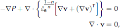
where P is a pressure deviation from hydrostatic (Reference BatchelorBatchelor, 1967, p. 176)for ![]() , is effective strain rate, v is the velocity vector with vertical component v and horizontal component u, and n is the power-law exponent. All variables (here and below, unless otherwise specified) are dimensionless. Gradients of the output velocities were used to determine the components of the dimensionless strain-rate tensor D, and corresponding components of the deviatoric stress tensor were computed with the constitutive relation:
, is effective strain rate, v is the velocity vector with vertical component v and horizontal component u, and n is the power-law exponent. All variables (here and below, unless otherwise specified) are dimensionless. Gradients of the output velocities were used to determine the components of the dimensionless strain-rate tensor D, and corresponding components of the deviatoric stress tensor were computed with the constitutive relation:
where B is the pre-factor in Glen’s flow law (Reference HookeHooke, 2005).
Since we are interested primarily in the sensitivity of ice flow to material properties and boundary conditions, the ice is assumed to be homogeneous and B is set everywhere to 1.
To generalize results and permit comparison with past modeling efforts, a simple two-dimensional rectangular domain scaled in units of ice thickness was used in initial model experiments (Fig. 2). The ice slab had no surface slope, and all flow was driven by an influx of ice into the domain from up-glacier. A second type of domain had an upper surface described by a parabola. Even for this domain, however, contributions to the stress field from local driving stresses were neglected, despite the sloping surface. This strategy allowed isolation of the impacts of longitudinal coupling on ice flow.
Fig. 2. Model domains and boundary conditions used in the finite-element simulations: (a) rectangular domain; (b) domain with parabolic upper surface; and (c) abrupt change in basal slip condition.
As illustrated in Figure 2, horizontal ice flow with depth-independent dimensionless velocity of 1 was prescribed along the left side of each domain. Ice was permitted to slip parallel to the bed for a portion of the bottom boundary up-glacier, but a transition to no slip was imposed down-glacier. An initial group of simulations was run with the same boundary conditions imposed by Reference Hutter and OlunloyoHutter and Olunloyo (1980), where ice was permitted to exit the domain only on the right-hand boundary. In these simulations, the upper boundary was shear-free, with zero normal velocity. In all other simulations, the upper boundary was prescribed to be stress-free. A consequence of the stress-free condition is that ice was free to exit the domain at the top where ablation was assumed to remove mass. For simplicity, a steady-state geometry was assumed, which required that ablation exactly match upward flow. This is not always a safe assumption, and its implications are addressed separately below.
The transition from slip to no-slip at the bed was enforced as an abrupt transition between no-shear stress and no-slip conditions at x = 0, much like the treatments of previous authors. Basal velocity at x = 0 was required to be zero, while the magnitude of the horizontal velocity at the neighboring node up-glacier was left free. Linear basis functions ensured that velocity gradients (and therefore stresses) were constant between nodes. With this in mind, discretization was guided by the notion that elements smaller than or roughly equal to the dimensions of the near-field plastic yielding zone (as defined above) would provide an upper bound for stresses. Realizing that most modern polythermal glacier termini are <200m thick at the BTT, using 1/200 as the minimum characteristic element size around the SNST ensured that stresses were bounded within the ~1m zone of enhanced plastic yielding. Stress fields obtained in this manner are viewed as more physically meaningful than those resulting from idealizations that assume step-change transitions, with associated stresses approaching infinity.
Domain geometries and meshes were created using the freely available mesh-generation software GMSH. Meshes ranged from a minimum of 5486 to a maximum of 27 156 linear, triangular elements. Pressure-velocity solutions were obtained first by solving the weak form of Equations (1) with three degrees of freedom at each node, u, v and P. The deviatoric stresses τxx, τyy and τxy were then computed directly from nodal velocity gradients. Note that there is no prescribed functional relationship between slip velocity and basal stresses. Solutions were obtained iteratively in each domain for ice with a power-law exponent n equal to 1, 2, 3 and 4.
Results
Each of the changes that were made to the geometry and conditions of the analytical SNST problem had a discernible effect on simulation results. The results are therefore presented as a series of changes to constraints, beginning with a reference simulation using the Reference Hutter and OlunloyoHutter and Olunloyo (1980) formulation. We then describe effects of relaxing constraints on boundary conditions, as well as domain geometry. While simulations were performed for a range of n values, our focus is mostly on results for n = 3. Changes in n were found to have minimal effects on kinematics and to mostly affect the magnitudes of stresses.
Results from a simulation of the SNST problem as originally formulated by Reference Hutter and OlunloyoHutter and Olunloyo (1980) are shown in Figure 3, including the analytical solution with n = 1 (equations 5.7 and 7.7 in Reference Hutter and OlunloyoHutter and Olunloyo, 1980) and finite-element solutions for n = 1 and n = 3. There is very good agreement between the Newtonian numerical and analytical solutions for velocities and stresses (Fig. 3c and d) both in the far field and near the SNST, indicating that the numerical approach gives accurate results. In the Newtonian case, ice does not begin to respond to the SNST until it is about two ice thicknesses away from the transition (Fig. 3c), at which point the basal velocity declines steeply, causing a concentration in basal shear stress at the SNST (Fig. 3d). While the analytical solution indicates stresses approaching infinity as x approaches 0, the corresponding numerical solution for n = 1 gives a finite peak shear stress at x = 0 (stresses are non-dimensionalized using the scheme of Reference CohenCohen, 2000). Due to confinement at the top of the domain, surface velocity increases over this region to conserve mass, reaching a steady surface speed within one ice thickness down-glacier of the SNST that is 33% larger than the up-glacier surface velocity (Fig. 3c). Numerical results for n = 3 show similar behavior, albeit with an even more subdued stress concentration (Fig. 3d) and a smaller increase in surface velocity beyond the SNST (Fig. 3c).
Fig. 3. Finite-element results of a reference simulation under boundary conditions employed by Reference Hutter and OlunloyoHutter and Olunloyo (1980) compared with their analytical results: (a) velocity vector field for n = 1; (b) velocity vector field for n = 3; (c) bed velocities from Hutter and Olunloyo’s n = 1 result (solid curve) and finite-element solutions for n = 1 (open circles show bed velocity; dash-dot line shows surface velocity) and n = 3 (dotted line shows bed velocity; dashed line shows surface velocity); and (d) bed shear stress from Hutter and Olunloyo (solid curve) and finite-element results for n = 1 (open circles) and n = 3 (dashed curve). The analytical results have been rescaled by a factor of 3 so that inflow velocity is 1 to facilitate direct comparison with later simulations.
We consider further only a power-law rheology (n = 3) and explore effects of allowing flow across the upper boundary and using a tapered (parabolic) domain geometry. These changes are introduced additively, with the final simulation including both effects and the power-law rheology.
Figure 4 summarizes representative finite-element results for flow over an abrupt transition in a rectangular domain, with a stress-free upper boundary and n = 3. At the extreme left-hand side of the domain, the ice feels the no-slip boundary far down-glacier (Fig. 4a and b). As a result, near-surface ice is deflected upward and across the top of the domain. The resulting loss of mass allows the remaining ice to proceed through the domain more slowly, accounting for the steady, nearly linear decline in basal velocity over most of the slipping portion of the bed (Fig. 4c). Because the bed in that region cannot support a shear stress (as required by the boundary condition), the horizontal surface velocity decreases almost identically. Only within about one-half of an ice thickness of the SNST is there a departure from this pattern. Here the basal velocity gradient steepens much like the near-field solution in analytical models. The result is a pronounced deviatoric stress gradient, for which we use bed shear and normal stresses as proxies (Fig. 4d). However, the reduced ice flux across the line x = 0 due to upward ice flow decreases the magnitude of the stress concentrations at the SNST by nearly 50% compared to the n = 3 case in Figure 3d. Horizontal and vertical surface velocities continue to decline gradually as ice passes over the SNST, eventually becoming nearly zero about two ice thicknesses beyond the SNST. In this zone of velocity decline, the horizontal and vertical surface velocity components are nearly equal, indicating that the ice-flow vector there is inclined approximately 458 from the bed (Fig. 4a). Down-glacier from there, ice is effectively stagnant because most of the inflow has already been lost to ablation.
Fig. 4. Results using a rectangular domain with an abrupt slip transition, n = 3, and an open (flow-through) upper boundary: (a) velocity vector field; (b) streamlines; (c) basal slip velocity (dotted curve), horizontal surface velocity (solid curve) and vertical velocity (dashed curve) (inset shows enlargement of the region around x = 0); and (d) basal shear stress (solid curve) and normal stress (dashed curve). Vertical scales in (a) and (b) are exaggerated.
Results for a simulation with an abrupt SNST and flow-through upper boundary are shown in Figure 5 for a domain with a parabolic upper boundary. Although qualitatively very similar to the results for the rectangular domain, there are subtle differences. A kinematic difference is that velocity components no longer establish linear trends in the sliding portion of the domain (Fig. 5c), owing to the down-glacier-changing surface slope. Nevertheless, as the ice approaches the SNST it is still deflected upward, as in the rectangular domain, producing a broad peak in upward velocity there, and again leaving a wedge of effectively stagnant ice at the terminus. Ice-flow vectors over the SNST are inclined somewhat less steeply than for the rectangular domain, and stress magnitudes exhibit peaks at x = 0 but remain small compared to the reference case (Fig. 3d).
Fig. 5. Results for a domain with a parabolic upper surface and abrupt slip transition, with n = 3: (a) velocity vector field; (b) streamlines; (c) basal slip velocity (dotted curve), horizontal surface velocity (solid curve) and emergence velocity (dashed curve), where emergence velocity is defined as v e =v+utan α, where α is the ice surface slope (inset shows enlargement of the region around x = 0); and (d) basal shear stress (solid curve) and normal stress (dashed curve). Vertical scales in (a) and (b) are exaggerated.
Simulations were also attempted using a prescribed function describing a continuous decline in basal velocity as a basal boundary condition. The smoothed sliding function further subdues stress concentrations but predicts untenable negative shear stresses in the sliding portion of the bed. Introducing gravity would likely eliminate these negative shear stresses but is beyond the scope of the present paper. Nevertheless, even with the prescribed smooth decline in basal velocity, ice flow is deflected toward the surface, leaving nearly stagnant ice at the terminus.
Discussion
The close correspondence between the numerical and analytical results for the test case shown in Figure 3 indicates that the finite-element method can reliably represent the macroscopic velocity and stress fields of interest. Additionally, in close proximity to the abrupt SNST, the numerical approximation limits stresses in a way that is consistent with the requirement that ice only supports finite deviatoric stresses. For example, the results presented in Figure 3d give a peak dimensionless shear stress at the SNST for n = 3 of approximately 3.58. When scaled to an arbitrary terminus thickness h 0 = 50 m, the characteristic element length used is 0.25 m, close to the lower end of Reference Van der VeenVan der Veen’s (1998) plastic-zone range. Further dimensionalizing (using the scheme of Reference CohenCohen, 2000) with reasonable values for B (30MPa s1/3) and inflow velocity u 0 (10ma–1), the peak dimensional shear stress is 0.099 MPa at the SNST, a good match with the commonly cited 0.1 MPa yield strength of ice (e.g. Reference PatersonPaterson, 1994, p. 188). Therefore, in this particular scaling example, the numerical solution represents near-field behavior around an abrupt SNST better than the analytical solutions. Further mesh refinement around the SNST is not only unnecessary but would give unphysical results. For significantly different values of scaling parameters, the mesh could readily be refined or coarsened around the SNST to bound the solution appropriately.
Each of the steps taken to relax constraints of analytical solutions has significant impacts on the velocity field. The most profound effect that can be seen by comparing either of Figures 4 and 5 with Figure 3 (n = 3) stems from allowing ice discharge out of the top of the domain. In each simulation described in Figures 4 and 5, ice-flow vectors acquire an upward component immediately upon entering the domain. This impact can be clearly attributed to the effect of discharge out of the domain on mass conservation. Ice entering the domain from up-glacier is deflected upward and out of the domain by slower-moving ice down-glacier. As a result, less ice needs to be conveyed further through the domain and down-glacier velocities decline. A change in the orientation of the upper surface across which mass is lost (i.e. use of a parabolic upper boundary) both lengthens that surface and reduces the vertical velocity component necessary to direct ice out of the domain. This changes the linearity of the longitudinal gradient in surface velocity as indicated by comparison of Figures 4c and 5c. The value of n has very little effect on the velocity field except in the local neighborhood (within three elements) of the SNST. Comparison of the velocity field for otherwise identical simulations indicates that outside of this zone a change from n = 1 to n = 4 produces changes in the velocity field of <5% of the inflow velocity. The lack of a significant influence of the value of n on the macroscopic velocity fields, combined with the conspicuous effects of changing upper and lower boundary conditions, indicates that conservation of mass subject to boundary constraints determines the velocity field much more than viscous deformation resistance. Had we allowed for a transient free surface and permitted ablation to inexactly compensate upward velocity, time-dependent evolution of the terminus geometry could have been calculated, but that calculation is beyond the scope of the present analysis.
The primary features of interest in the simulated stress fields are the magnitude and distribution of deviatoric stresses induced by the SNST. Each of the steps taken in relaxing model constraints (Figs 3–5) reduces the magnitude of the basal shear stress peak. In particular, allowing ice flow across the upper boundary causes significant stress reduction. Upward ice flow, balanced by ablation, decreases velocity gradients by reducing total horizontal ice flux. The magnitude and distribution of deviatoric stresses on the bed would also be affected by the smoothing of basal velocity. While the peak in basal deviatoric normal stress (which is the opposite of longitudinal stress in plane strain and therefore an indication of longitudinal stress transfer) occurs sharply at an abrupt SNST, it would be broadened for a smoother transition and focused not where slip velocity nears zero but where the slip velocity gradient is greatest.
Allowing for non-zero basal shear stresses and a consequent departure from plug flow in the freely sliding portion of the model glacier would further improve realism. For example, if we were to allow slip velocity in the model to adjust to basal stresses through an effective-stress dependent slip law (e.g. equation 21 of Reference PatersonPaterson, 1994, p. 151), the enhanced normal stress on the bed up-glacier of the BTT (Figs 4d and 5d) would contribute to smoothing of the basal velocity transition. Also, inclusion of local driving stresses (gravity) could potentially influence results with the parabolic upper surface. Small but discernible effects of gravity are likely (e.g. the volume of nearly stagnant ice at the margin might be reduced by superposition of simple shear driven by the downslope component of the glacier weight). However, a major influence of gravity on our results would not be likely, given the generally large deviatoric stresses associated with longitudinal stress transfer at the BTT, relative to those associated with the local glacier weight.
Implications
These results suggest that reliance on existing analytical models of SNSTs may lead, among other things, to overestimation of the importance of thrusting in glacier margins. Longitudinal compression across the BTT of a frozen margin deflects ice away from the bed, enhancing upward ice flow and, upon ablation, removes it from the system. In three dimensions, a transition from temperate-based ice to cold-based ice is almost certainly irregular or patchy. Even where local velocity gradients are steep, strain heating would extend the zone of soft temperate ice. If stresses did manage to reach a threshold level, plastic yield would accommodate strain. Each of these processes would tend to broaden the transition from sliding to non-sliding ice, thereby reducing the magnitude of stress concentrations. Without an extraordinary stress concentration, ice in typical glaciological environments will not behave in a brittle manner under compression (Reference SchulsonSchulson, 2002).
Inspection of velocity vectors and streamlines in Figures 4 and 5 indicates that objects initially near the bed in the sliding portion of a glacier would eventually emerge at the surface within a few ice thicknesses of the BTT. Planar englacial features initially oriented parallel to streamlines would be rotated along with the streamlines as they were passively transported down-glacier, attaining dips as large as 458. Because boundary conditions prevent basal drag in the sliding segments, the dominant component of the strain field up-glacier of the BTT is horizontal shortening and vertical extension (pure shear). Under this regime, pre-existing features oriented at an angle to streamlines would steepen as they move toward the BTT and the surface, as indicated in Figure 6. An initially slightly inclined structure deep in the ice (e.g. a basally accreted sediment lens) would become rotated to steeper angles by the time it outcropped at the glacier surface (cf. Reference Hooke and HudlestonHooke and Hudleston, 1978). The addition of a bed-parallel simple shear component arising from inclusion of gravity could counteract this rotation to some degree if it were large compared to the longitudinal compressive stresses. Nevertheless, upward deflection and substantial rotation of structural features formed at depth within the glacier (such as debris bands in basal ice) may be explained by continuum flow in the vicinity of a SNST. This provides a mechanism for generating thrust-like structures in ice margins without appealing to uplift along a structural discontinuity.
Fig. 6. Progressive deformation of a passive marker in the simulation shown in Figure 5, assuming a steady state. A slightly convex-up, sub-horizontal structure that is initially 0.04 ice thicknesses above the bed is rotated up-glacier, longitudinally shortened, and vertically extended as it approaches the SNST and is deflected toward the surface. Vertical exaggeration is 2 and the dimensionless time-step is 2h 0 /u 0.
Finally, in most of our simulations, ice more than two ice thicknesses down-glacier from the SNST is largely stagnant, a result that contrasts greatly with the down-glacier speedup predicted in earlier models that prevent ice flow out the top of the domain. Assuming that ablation rates are roughly constant along a flowline or vary linearly with surface elevation, a geometry such as the parabolic profile of Figure 5 would not be sustainable. The nearly stagnant ice at the terminus would melt away, unless insulation there provided by surface debris or snow inhibited ablation sufficiently. Alternatively, if ablation was sufficient to balance upward ice flux in the slow-moving terminus but was unable to keep pace with faster upward flow immediately up-glacier, a bulge would form in the ice surface in the vicinity of the BTT. A number of polythermal surge-type glaciers do develop such bulges near their surge fronts, which in some cases appear to be coincident with their basal thermal transitions (e.g. Reference Clarke and BlakeClarke and Blake, 1991; Reference Fowler, Murray and NgFowler and others, 2001).
Conclusions
Our numerical model builds on previous analytical models of SNSTs by using a power-law rheology, realistic terminus geometry, allowing ice loss (ablation) from the top of the model domain, and eliminating singularities in basal stresses. Under these more realistic constraints, model results indicate that longitudinal compression at the BTT is accommodated by vertical extension, resulting in uplift of ice from depth and a down-glacier decline in surface velocity. Upwardly deflected flow can account for the appearance at the glacier surface of up-glacier-dipping structures containing basal sediment even in the absence of thrusting along discontinuities. Thrusting is further disfavored when account is taken of the numerous processes that likely contribute to limiting stress magnitudes. Results also suggest that an imbalance between the spatial patterns of upward ice velocity and ablation rate can lead to very different terminus geometries. Further development of this model will include introducing gravity, allowing rheological heterogeneity in the ice, and tracking the evolution of the free surface under various imposed ablation patterns. Work is underway to apply this strategy to the terminus of a polythermal glacier (Storglaciaären, Sweden) to help understand the effects of its frozen margin on terminus structure and behavior.
Acknowledgements
We thank R. Hindmarsh for an insightful review of an earlier draft of this paper. O. Gagliardini, J. Ruokolainen and T. Zwinger assisted with model implementation. This work was supported by a grant from the US National Science Foundation (EAR-0541918).

