

Introduction
Topographic maps contain a lot of information about the different phenomena that can affect an ice sheet. At large scale (>1000km), ice-sheet size and shape are controlled by climatic and dynamic processes and by boundary conditions. Several processes also act on the medium (100 to >1000 km) and small scale (1 to > 100 km): anisotropy, longitudinal stress, bedrock geometry, basal sliding, etc. Each of these processes has its own effect on the surface of the ice sheet. Due to the precision of satellite altimetry, we are better able to determine the effects of these processes on the surface topography. The problem lies in separating and explaining their different signatures.
Some authors already use the surface topography to estimate rheological parameters (Reference Young, Goodwin, Hazelton and ThwaitesYoung and others, 1989; Reference Remy, Ritz and BrissetRemy and others, 1996), but these data alone are not sufficient. One of the major limitations when topography is used to test or constrain flow models is the lack of precise bedrock topography. Recently, during an Italian expedition inTerre Adelie, ice-thickness measurements were performed along a 1200 km traverse between Terra Nova Bay and Dome Concordia (Dome C) (Fig. 1). The aim of this paper is to develop a classical ice-sheet model and to use precise geometrical boundary data to better understand the ice-flow processes.

Fig. 1. East Antarctica from 90°–180° E. Contours begin at 82° S. Contour interval is 130 m. The thick line corresponds to the flight traverse carried out in January 1997 from the Terra Nova Bay Italian base (164.1° E, 74.69° S) to Dome C (75.1° E, 123.38° S). The limits of each leg are indicated by black points.
Data
Ice-thickness data were obtained by radio-echo sounding from an airborne radar of 60 MHz frequency. These data were then combined with an interpolated profile from European Remote-sensing Satellite (ERS-1) altimetry. After smoothing and digitization, a file of bedrock elevation for every 1km along the 1160 km profile was produced, with a mean vertical precision of about 10 m. Comparison of this bedrock profile with the interpolated bedrock from the Scott Polar Research Institute (SPRI) glaciological and geophysical folio (Reference Drewry, Jordan and DrewryDrewry and Jordan, 1983) shows large differences at the small scale: in some places the two profiles differ by more than 400 m (Fig. 2).
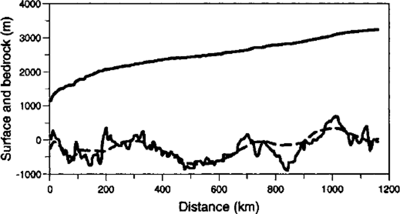
Fig. 2. Surface and bedrock geometry from Terra Nova Bay (km 0) to Dome C (km 1160). Surface is from ERS-1 altimetry. Solid bedrock from traverse radio-echo soundings. The dashed line correspond to the bedrock interpolated from Reference Drewry, Jordan and DrewryDrewry and Jordan (1983).
The very dense sampling of the geodesic cycle of the ERS-1 altimetric mission allows us to recover the surface topography with a very high spatial resolution. Reference Remy and TabaccoRemy and others (in pres) analysed 30 million waveforms of altimetric data over Antarctica to compute maps on a 1/30° grid. The estimated elevation precision of this high-resolution topography is around 30 cm rms at crossover points.
We calculate the angle between our profile and the flow direction represented by the local slope (averaged over 10 km). The mean value of this angle for the total flight is 20°. The greatest values (>45°) are localized between km 190 and 350, along the profile this occurs some 200 km upstream of the 90° turning of the flight (see Fig. 1). Except for this section, the profile mainly follows the steepest slope direction and the plateau does not exhibit strong convergence or divergence zones.
Theoretical Basis
Equations
We assume the "shallow-ice approximation" and a power-creep law for the behaviour of the ice which gives the depth-averaged deformation velocity, Ud, as a function of thickness, H, and basal shear stress, τ, to the power n. We will use here the analytical expression of Reference LliboutryLliboutry (1981):

B(T) is the function of how the ice deformation depends on ice temperature via an Arrhenius-type relation with ![]() and p = n - 1 + kGH. Here G is the bottom temperature gradient taken as 0.022°C m−1 corresponding to a 50 mW m−2 geothermic flux, Tb is the mean bottom temperature, Tm is the melting temperature at the bottom of the ice sheet (Tm = 273 - H/1503 expressed in R Q is the activation energy for creep taken as 60 kJ mol−1, R is the universal gas constant (8.31 J mol−1 K−1), p is the density of ice, g is the gravitational constant and B0 the flow-law coefficient which seems to depends on crystal structure, orientation of the c axes and impurity concentration.
and p = n - 1 + kGH. Here G is the bottom temperature gradient taken as 0.022°C m−1 corresponding to a 50 mW m−2 geothermic flux, Tb is the mean bottom temperature, Tm is the melting temperature at the bottom of the ice sheet (Tm = 273 - H/1503 expressed in R Q is the activation energy for creep taken as 60 kJ mol−1, R is the universal gas constant (8.31 J mol−1 K−1), p is the density of ice, g is the gravitational constant and B0 the flow-law coefficient which seems to depends on crystal structure, orientation of the c axes and impurity concentration.
Lliboutry obtained Equation (3) from an analytical integration of du/dz based on a relation between temperature and depth. The error due to this analytical integration with respect to a numerical integration is less than 1 %. The only major assumptions are that the rheological parameters B0, n and Q are constant through the ice thickness.
For steady-state flow with neither convergence nor divergence, the balance velocity Ub is given by
where b is the accumulation rate.
Assuming equality of these two velocities we have, from previous equations, a relation between the thickness and the shear stress:
where f is the accumulation integral divided by B(T).
Most models are based on some form of these relations. Although the flow law is well supported by mechanical experiments, its use in models poses a few problems (Reference AlleyAlley, 1992). The different parameters n, B0 and Q have a large set of empirical values which can vary with the state of the ice (temperature, viscosity, strain rate, types of creep, etc.). The scale of calculation of the shear stress is also a "parameter" which can have an influence on the validity of the law. In this paper we endeavour to use the precision of our data to estimate these different parameters.
Input values
Spatial scale for calculating the slope
The surface slope and its direction play a role in estimating the magnitude and direction of ice flow. Due to the presence of undulations at the 10 km scale, the length of smoothing of the topography is critical. Many authors (Reference PatersonPaterson, 1981; Reference Cooper, Mclntyre and RobinCooper and others 1982; Reference Young, Goodwin, Hazelton and ThwaitesYoung and others, 1989) suggest using a 50 km scale when calculating the shear stress to smooth the effects of the longitudinal stresses. Investigations on the influence of spatial smoothing with our data led to the same result. In this study we will use the surface slope calculated from the ERS-1 altimetric surface by linear regression at each point at a scale of 20 times the thickness. Using this smoothing, Figure 3b shows the variation of basal shear stress along the Terra Nova Bay-Dome C profile.

Fig. 3. Quantities involved in the theory from Terra Nova Bay (km 0) to Dome C (km 1160): (a) Basal temperature estimated from the thermodynamic equation (solid line) and the basal melting temperature correction (dashed line); ( b) shear stress calculated at a 20 times thickness scale from the ERS-1 geodetic topography; and (c) strain rate calculated from balance velocity and thickness.
Accumulation rate, basal temperature and shear strain rate
Accumulation rates are interpolated along the profile using maps from Reference Radok, Jenssen and MclnnesRadok and others (1987). The bottom temperature (Fig. 3a) is estimated from the thermodynamic equation under a steady-state assumption and considering dissipation, vertical diffusion, vertical and horizontal advection. More details can be found in Reference RitzRitz (1987), Reference Remy, Ritz and BrissetRemy and others (1996) or Reference Remy and MinsterRemy and Minster (1993). The quantity U/ H derived from balance velocities and the thickness is supposed to be proportional to the mean shear strain rate ε through the ice thickness (Fig. 3a). We will use a "temperature-dependent shear strain-rate" ε′ = (p + 2)U b/H exp[k(T b – T m)] in this paper. With this notation the Glen flow law can be written:
Estimation of the Parameters
For a flow law invariable along the profile
Assuming that the parameters involved in the flow law (n, B0, Q, spatial scale of shear-stress calculation, etc.) are constant along the profile, linear regression between r and ε’ for the whole profile provides a statistical estimation of the parameters n and B0, with n = 1.5 and B 0 = 0.3 ba−1.5 a"1 and a correlation coefficient of r = 0.42. The influence of the n in the p parameter (see Equation (3)) is negligible for the regression. These n and B0 values are consistent with those found in the literature.
We now compare the along-profile variations of the two terms of Equation (5) to examine the validity of our hypothesis and of the flow law with all the parameters (calculated or estimated). Comparison of these two quantities (Fig. 4) shows strong discrepancies. If we focus on the part of the profile which corresponds to the plateau (i.e. after km 200), we see that the righthand term decreases slowly up-flow, representing the decreasing value of the accumulation-rate integral. On the contrary, the lefthand term, H2Tn shows an up-flow trend of either increasing magnitude (n = 1) or constant trend (n = 3). Any feasible estimation of the accumulation rate, or of the bottom temperature, cannot explain this difference. To explain such discrepancies both a positive bottom temperature from 200 to >500km and a temperature decreasing from –10°C to –60°C from 700–1160 km would be needed. For the accumulation-rate integral similarly unrealistic values are needed, diminishing by a factor 10 from km 900 (near Dome C) to km 200 (edge of the plateau).

Fig. 4. Comparison of the left and right term of Equation (5) in 10 6 m2 bar". Solid line corresponds to the righthand term and is equal to the integral of accumulation rate divided by B(T). The three others curves correspond to H2Tn for n=l,2 and 3, respectively.
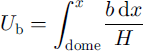
This difference may be explained if the flow-law coefficient B0 has a variation of a factor of 100 and the same global trend as the sum of accumulation rate (see Equation (5) and Fig. 4). It is difficult to asses the evolution of B0 along the profile since its behaviour depends on various factors or complex processes (fabric, grain-size, impurities, anisotropy, orientation of the c axes, strain, etc.). However, the large-scale trend of B0 is qualitatively in agreement with Reference Pimienta and DuvalPimienta and Duval (1987) who note that as the flow increases, a strongly oriented fabric develops, which in turn enhances the flow. Figure 5 shows the magnitude of B0 required to satisfy Equation (5) (with n = 1.5).
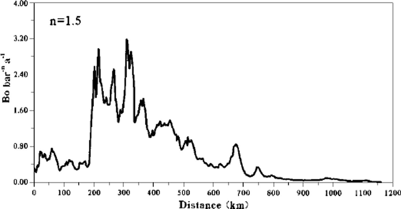
Fig. 5. Magnitude ofB0 ( bar-n a–1) needed to satisfy Equation (5).
For a flow law which varies with the location
Figure 6a shows the shear stress, τ, versus the temperature-dependent shear strain rate ε’. Values of n and B0 can be calculated from the slope of the points in this plot. Using a linear regression with a 100 km wide window, the parameters B0 and n were calculated each kilometre from km 50 to km 1110 (Fig. 7). From these two figures we can see that the observed behaviour of the ice along the 1160 km long profile is more complicated than can be explained by a constant flow law. In spite of the apparent confusion of points in Figure 6a, some significant features can be observed. Most important is that the flow law seems to be valid over distinct segments. Five separate areas show a consistent value of n (Fig. 7), each of them corresponding to a maximum of correlation. The mean values of n and B0 for each of these intervals with their associated correlation, r, are given below.

Fig. 6. (a) logT(bar) vs log ε’ (a−1), (b) Bedrock geometry (solid line) and surface slop ε (dashed line). (c) Path of the profile on contour elevation map. Below 2300 m (bold contour) the contours are each 15 m, above 2300 m contour interval is 5 m.
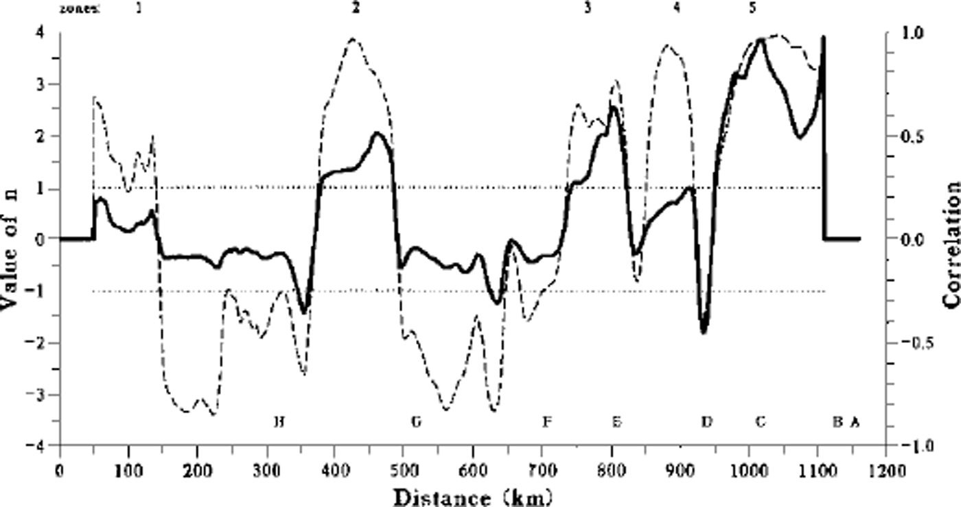
Fig. 7. Linear regression between log τ and loge’ each km along the profile with a 100 km window. The solid line corresponds to the Glen flow exponent (i.e. regression coefficient) and the dashed line to the correlation coefficient, r, of the regression (right scale). Dotted lines indicate significant correlation at the 99% confidence level.
We consider that the first 350 km does not fit our hypothesis, because zone 1 is a convergence zone and at the beginning of the plateau the profile from 190 to 350 km is not aligned in the flow direction.
With the exception of zone 4 (discussed below), the n value seems to increase from the coast to Dome G. Reference Remy, Ritz and BrissetRemy and others (1996) found a value of n around 1 for temperatures less than –10°C and increasing n values for warmer temperatures. One can see from Figures 3a and 7 that the large-scale behaviour of n and Tb is similar from km 200 to Dome G.
Discussion
It is obvious from Figure 6 that, even if a classic law can be applied regionally, it is not able to explain all the topographic features observed. However, some of the observed discrepancies can be isolated and explained by local physical phenomena.
Sliding
Reference Siegert and RidleySiegert and Ridley (1998), using an analysis of radio-echo sounding, show that the flat-surface region (133° E, 73–74° S) lying over the Adventure Subglacial Trench had a relatively bright return from the ice substrate, but no mirror-like reflection. They conclude that water is not trapped within a subglacial hollow and infer that the transport of water probably occurs through an unknown basal hydrological system. This is probably the channel that is crossed by our profile at km 850. This region corresponds to a maximum in thickness (>3700 m) and should have a positive basal temperature (Fig. 3a). A careful examination of the surface topography of this region (between D and E in Fig. 6c) shows a flatter zone. There is also a 10–20 km wide channel in the topography at the eastern border of the flatter zone which reaches the Adventure Subglacial Trench and could mark the position of the subglacial hydrological system. The occurrence of sliding produces a flatter surface and could explain the strong diminution of τ (between D and E in Fig. 6a) and the low value of n in zone 4.
Local sliding could also partly explain the anomalies observed between points C and D and between points Fand G where negative values of n are found (Fig. 7). In particular, these anomalies occur when there is a decrease of τ at constant ε’ which seems to correspond to basal sliding (see above between D and E). The presence of relatively high radar-echo reflectivity in both cases (in spite of negative temperature, Fig. 3a) suggests the presence of water at the bottom of the ice. Local phenomena such as enhanced geothermal flux or strain dissipation could generate the right conditions for the existence of water in the ice. This also applies for local anomalies from the flow law in the Dome C region (for instance in Figure 6a between km 1123 and 1135 where τ decreases between points A and B). This behaviour could be a consequence of the subglacial channels which occur beneath Dome C (Reference Remy, Shaeffer and LegresyRemy and Tabacco, 1999).
Anisotropy
Anisotropy is suggested by Figure 6a between points G →H and E → F (or between zones 2 and 3). At large scale, zones 2 and 3 have the same behaviour with a mean slope around 1.5 but we observe a clear shift between them. Although the ice is subject to shear stress of the same order of magnitude and the temperature is taken into account in ε’, these two zones show strong differences in the intensity of the shear strain rate. Changes in the ice-crystal-orientation fabric between these two regions can lead to such behaviour, and correspond to a change of B0.
In our case, B0 is enhanced by a factor of 4.4. Reference Jacka and BuddJacka and Budd (1989) found that in isotropic ice the development of anisotropy leads to an enhancement factor of 3 when isotropic ice is subject to compression and a factor 8 in shear. Reference Remy, Ritz and BrissetRemy and others (1996) found an enhancement factor of 3.
Longitudinal stress
A loop is observed between km 650 and km 800 which perturbs the estimation of n in zone 3 and explains the low value of r. This is due to the fact that in this region τ and ε’ vary in a similar way, but with a shift of 20 km. A look at this region on the surface map shows that the profile crosses a flat zone, but the estimation of basal temperature in this region is about –5°C, and the depression in the bedrock does not give a strong radar echo. A small trough followed by a bump of 2 m amplitude is observed at km 740 in the topography. This kind of signature is also observed in the transition zone between strong friction and weak friction in the Lake Vostok area and was quantitatively attributed to the effect of longitudinal stress (Reference Remy, Shaeffer and LegresyRemy and others, 1999). Therefore, this loop could be a residual effect of longitudinal-stress gradients which have not been entirely smoothed.
Conclusion
The use of a simple model based on the Glen flow law coupled with precise boundary datasets along a 1160 km profile allowed us: to test the validity of the law; to estimate the variation of the ice-flow parameters; and to link some of the anomalies with physical processes.
The major result is in determining the non-unique nature of the flow law and/or the non-constancy of its rheological parameters along the profile. Assuming a unique law with constant parameters leads to discrepancies which cannot be explained with reasonable assumptions. On the contrary, if the rheological parameters n and B0 averaged over a 100 km scale are assumed to vary freely, n is found to vary discontinuously, but on average increases from the coast to Dome C, probably linked to the increase in basal temperature. Moreover, the different physical processes (sliding, anisotropy, longitudinal stress) involved in some of these discrepancies might be isolated by their expected effect on n and B0.
A precise knowledge of the geometric flow boundary can contribute significantly to ice-flow modelling via a better constraint of the bottom and surface topography, an estimation of the model parameters, and a better description of the signature of anisotropy, sliding or longitudinal stress. The modelling of these mechanical processes could thus be improved or tested.
Acknowledgements
We thank B. Legresy for his help and numerous discussion and the two referees for their comments. This paper is the result of a Franco-Italian collaboration, supported by an European Science Foundation (ESF) grant, within the European Ice Sheet Modelling Initiative and it is a contribution to the "European Project for Ice Coring in Antarctica", ajoint ESF (European Science Foundation)/European Commission (EC) scientific programme, funded by the EC under the Environment and Climate (1995–98) contract ENV4-CT95-0074 and by national contributions from Belgium, Denmark, France, Germany, Italy, The Netherlands, Norway, Switzerland and the United Kingdom.


