Introduction

The Soil Moisture and Ocean Salinity (SMOS) satellite is the European Space Agency’s (ESA) second Earth Explorer Opportunity mission (see http://www.esa.int/livingplanet/smos). SMOS will carry an L-band (1.4 GHz, or 23 cm wavelength) microwave radiometer into space, with the primary objective of making measurements of terrestrial near-surface soil moisture and ocean surface salinity. Since SMOS will be launched on a polar orbiting platform, it also has a secondary objective to perform cryospheric measurements over land and sea ice. SMOS launch is planned for 2007.

L-band radiometric measurements of the properties described above require a very high level of radiometric fidelity and accuracy to be able to sense subtle brightness-temperature variations. As a result, to be of any practical value, external geophysical control targets must undergo either smaller or predictable changes in their emissivity and thermal forcing.

The size, structure, spatial homogeneity and temporal thermal stability of the high-elevation Antarctic plateaux, such as at Dome C (75˚06’06’’ S, 123˚23’42’’ E), make such locations prospective candidates for the external calibration or validation of satellite-borne microwave radiometer brightness-temperature products. However, few, if any, experimental measurements of ice-sheet surfaces are available. Thus, the purpose of this paper is to assemble information with which to assess the suitability of the target as an external calibration target. Of particular interest are the temporal stability of the L-band emission and the uniformity of the target. To date, the Skylab S193 measurements (Reference Lerner and HollingerLerner and Hollinger, 1977) are the only space-borne L-band radiometer data, but they are limited by the 50˚ orbit inclination of the space station. Thus, as far as the authors are aware, experimental L-band observations of ice sheets are not available, so historical microwave measurement data at other frequencies are used in the following section to characterize the expected variability in this frequency range. We attempt to reproduce these satellite data using physically based electromagnetic modelling tools, and to extrapolate results to the L-band SMOS measurement waveband. Finally we briefly treat the ionosphere, which can have a perturbing effect on the satellite-borne radiometer measurements.

Satellite Observations

Satellite microwave radiometer data from NASA’s Scanning Multichannel Microwave Radiometer (SMMR) and the US Department of Defense’s Special Sensor Microwave/Imager (SSM/I) provide a unique 20 year dual-polarized, spectral record of Antarctic brightness temperatures that prove invaluable for seasonal to interannual investigations of ice-sheet surface properties (Reference RottRott, 1990; Reference SurdykSurdyk and Fily, 1993; Reference Bingham and DrinkwaterBingham and Drinkwater, 2000). In Figure 1, calibrated, multi-channel brightness temperature (T _b) data are plotted from SMMR and SSM/I for the period 1978–2001 (Reference Jezek, Merry and CavalieriJezek and others, 1993). V-polarized T _b values are selected here for illustrative purposes, although H-polarization is noted to have greater sensitivity to seasonal variations in roughness and other surface effects. The typical differences in seasonal amplitude between V- and H-pol T _b values are 0.5, 1.9, 1.7 K at 37, 18/19 and 5 GHz, respectively.

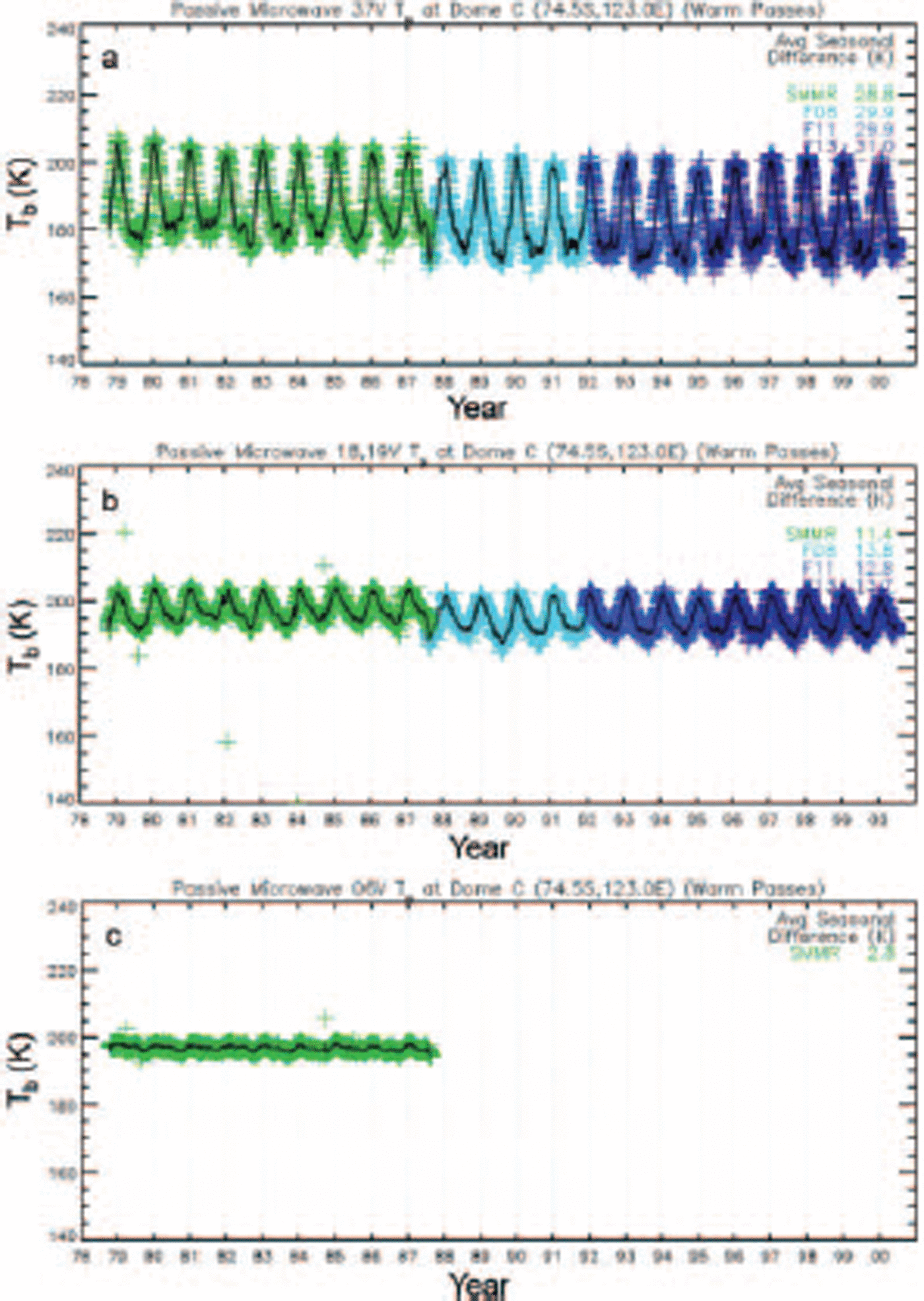
Fig. 1. Satellite microwave brightness temperature TB (V-pol) time series measured at Dome C by the series of Defense Meteorological Satellite Program (DMSP) satellite-borne (F08, F11, F13) SSM/I instruments and the Nimbus-7 SMMR instrument at 37GHz (a), 18/ 19GHz (b) and 6.6GHz (c), over the period 1978–2001 (courtesy US National Snow and Ice Data Center (NSIDC)).

Though the SMMR values have been adjusted according to the method proposed by Reference Jezek, Merry and CavalieriJezek and others (1993), residual calibration inaccuracies, together with differences in sensor characteristics, explain the step observed in 1987 at the boundary between SMMR and SSM/I datasets in Figure 1a and b. The time series in Figure 1b, for instance, experiences a

Figure 1 examples clearly indicate that the amplitude of annual T _b variations at Dome C decreases (increases) with increasing wavelength (frequency) in a manner consistent with previous SMMR observations made at other locations (Reference RottRott, 1990). Various authors tested hypotheses to explain this phenomenon (Reference Van der Veen and JezekVan der Veen and Jezek, 1993; Reference Bingham and DrinkwaterBingham and Drinkwater, 2000). Each concludes that longer wavelengths penetrate cold, dry firn more effectively (experiencing less scattering loss from snow grains and a loss factor of ice that is only weakly frequency-dependent). Reference RottRott (1990) estimated frequency-dependent penetration depths directly from SMMR V-polarized data at Plateau Station, East Antarctica, obtaining values of 0.9, 4.0, 11.5 and 18m for 37, 18, 10.7 and 6.6 GHz, respectively. Together, these results suggest that longer-wavelength seasonal T _b variability is driven by thermal cycles that are increasingly damped with respect to surface atmospheric temperature forcing. At the higher frequencies, due to the smaller penetration depths the thermal emission is confined to the surface layers where the thermal variability is greatest. In contrast, below 10m depth, the annual cycle has virtually disappeared and the variation of the firn temperature becomes negligible. Thus, over the 10 year period 1978–87, C-band emissivity at depth is extremely stable.

Figure 2 indicates 23 year mean seasonal peak-to-peak differences extracted from all SMMR and SSM/I channels at Dome C. Values diminish with decreasing frequency from 30 K at 37 GHz (Ka-band), to around 3 K at 6.6 GHz (C-band), according to the empirical relationship y=0.191x ^1.4, where y is the seasonal range and x is the frequency v (in GHz). When extrapolated to L-band, this frequency-dependent relationship suggests that the seasonal range of variation is likely to be significantly smaller than 1 K. C-band results in Figure 1 already confirm that Dome C is extremely stable on satellite mission duration time-scales of several years. This makes Dome C an appropriate target for SMOS external calibration and checking for drift in instrument calibration. In order to investigate this further, we conduct an electromagnetic model simulation in the following section both to confirm these findings and to qualitatively assess the impact of physical variability on L-band radiometer measurements.

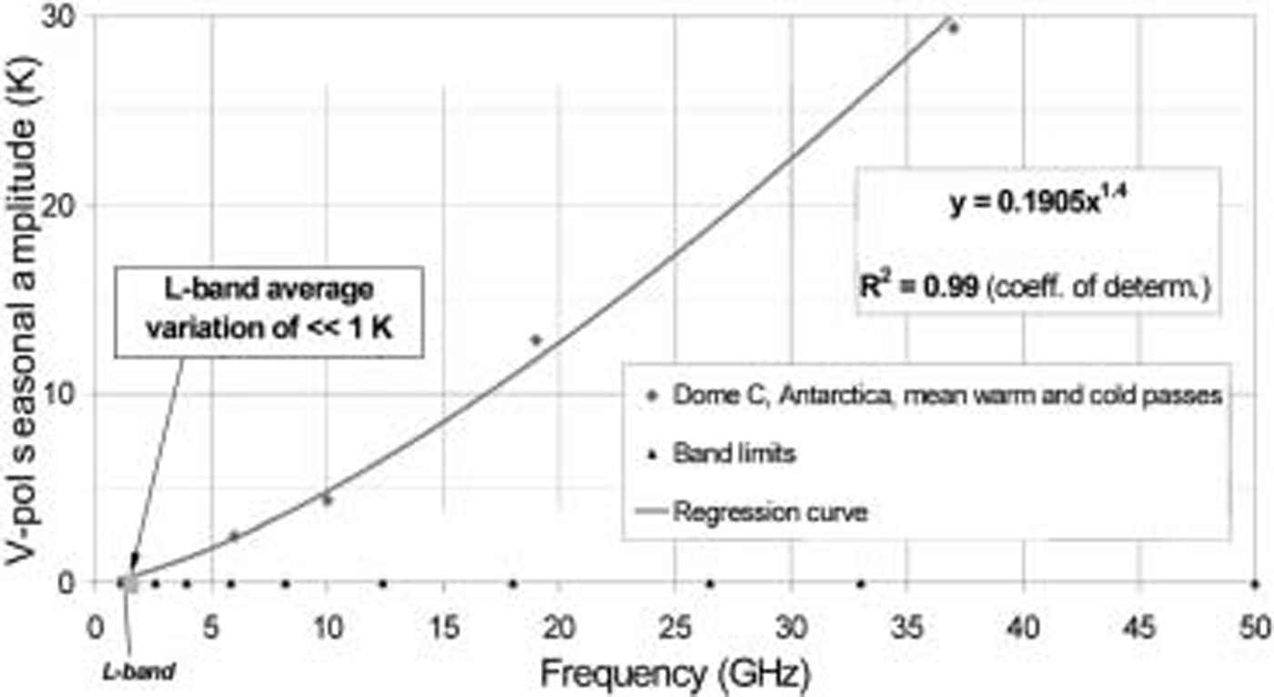
Fig. 2. Frequency dependence of the observed mean seasonal variation in brightness temperatures measured at Dome C during 22 years (1978–2000) of multi-channel passive microwave data from SMMR and SSM/I.

A Model for L-Band Emission

We investigate the microwave emission at Dome C further using a physically based, multi-layer electromagnetic model MIMESI-MC (MIcrowave Model for Emission of Snow Ifac – Multilayer Coherent). The approach follows methods used in recent L-band simulations of Dome C emissivity made by C. Mätzler (personal communication, 2001) using previously documented models (Reference Mätzler and WiesmannMätzler and Wiesmann, 1999; Reference Mätzler, Wiesmann, Pulliainen and HallikainenMätzler and others, 2000; Reference Wiesmann, Fierz and MätzlerWiesmann and others, 2000). In MIMESI-MC, the reflection and transmission wave amplitudes are computed for a layered medium following the wave approach (Reference KongKong, 1990). The ice-sheet medium is divided into n layers with boundaries whose separation and depth is configurable on the basis of available in situ data. A top layer is bounded by the air/snow interface, while the bottom (n+1)th layer is considered semi-infinite in depth. Effective permittivity is computed for each layer using strong fluctuation theory. The reflection coefficient is expressed in a recurrent relationship, and the amplitudes of waves in each layer are obtained by using the propagating matrices (Reference KongKong, 1990). Using the fluctuation dissipation theorem (Reference JinJin, 1984), brightness temperatures at V- and H-pol are then expressed as the sum of contributions from all individual layers.

The emission of a mixture of ice and air is driven by the vertical distribution of layering, which can be characterized by two major parameters:

the effective complex dielectric constant, which determines a layer’s ability to emit and attenuate electromagnetic waves; and

the physical temperature, which directly affects the relationship between emissivity and brightness temperature and which drives to a certain extent the imaginary part of the dielectric constant.

The former is governed by the physical structure of the medium and by its physical temperature, while the latter results from external surface temperature forcing and the extent to which penetration of the seasonal temperature wave is governed by the thermal conductivity of the layers.

L-Band Simulation Results

The model described above is used to investigate the impact of variations in physical properties on the electromagnetic interactions with the layered snow/firn and ice at Dome C. The model specifies the number and thickness of each layer as a function of depth z. Layer properties were specified as a function of frequency and temperature using a procedure similar to Reference Bingham and DrinkwaterBingham and Drinkwater (2000) and Reference Floury, Drinkwater and WitasseFloury and others (2002). The primary difference is that the effective permittivity for each layer was computed by using strong fluctuation theory on the basis of depth-dependent fractional volume, grain-size and correlation length.

The European Project for Ice Coring in Antarctica (EPICA) has obtained a depth profile of density and mean particle size that is used to prescribe layer physical properties in the model (see: http://www.pangea.de/Projects/EPICA). The mean accumulation rate at Dome C is around 3.7cma^–1 w.e., and the surface density is around 300 kg m^–3, leading to surface layers around 12cm thick that decrease as a function of depth z and firn density. The firn density ρ(z) is assumed to increase exponentially with depth. Following Reference Bingham and DrinkwaterBingham and Drinkwater (2000) we used the empirical depth-dependent density relationship

(1)

with ρ(z) expressed in g cm^–3 (10³ kg m^–3). This density behaviour has been compared with profile measurements from the Dome C EPICA project (Reference BarnesBarnes, 2002): a comparison made between simulated and measured profiles indicates good agreement. Settling and packing of grains in the upper surface snow results in a strong gradient of density down to depths of around 5 m. Beyond this depth, the firn density typically exceeds 421 kg m^–3 (i.e. a volume fraction of 0.46) and increases more slowly as interconnecting airways close off and bubbles form. By 100m depth and below, the density typically exceeds 800 kgm^–3.

Among the factors that strongly influence microwave emission of snow and firn are the size and morphology of grains including size distribution, shape anisotropy, grain morphology and topological characteristics. Polar ice experiences grain growth through time. Normally, grain growth occurs as a linear increase in cross-sectional area C with time t, expressed as

(2)

where C ₀ is the mean cross-sectional area at time zero and K(T) is a crystal growth rate (with typical value of 0.00042 mm² a^–1) exhibiting an Arrhenius dependence on temperature T Reference Gow(Gow, 1969). The evolution of mean grain-size as a function of depth for the EPICA ice core is reported in Reference GayGay (1999), Reference Arnaud, Weiss, Gay and DuvalArnaud and others (2000) and Reference BarnesBarnes (2002), while shallow measurement data are available in Reference Gay, Fily, Genthon, Frezzotti, Oerter and WintherGay and others (2002). A linear regression of mean crystal-size data between 100 and 430m seems to be reasonable, but for deeper ice (430–500 m) the mean crystal area was observed to decrease significantly. This decrease in mean crystal size has been observed in the old Dome C (74˚39’ S, 124˚10’ E; elevation 3240 m) and several other ice cores, and is associated with recrystallization as a result of the ice flow.

Surface temperature forcing is prescribed using a 10 year mean seasonal cycle fitted to Dome C automatic weather station (AWS) records (after Reference Bingham and DrinkwaterBingham and Drinkwater, 2000). Conventional heat conduction theory is then employed to calculate the seasonally dependent vertical temperature profile in the model upper layers. The thermal diffusivity of snow k is calculated as a function of the thermal conductivity K _s and the specific heat capacity γ.

Fig. 3. (a) Model simulated snapshot of L-band brightness temperature as a function of incidence angle at Dome C during January; (b) the depth-dependent contribution of each of the layers to the brightness temperature, over the depth interval 0–800 m.

(3)

The thermal conductivity of each layer is computed as a function of its density following Reference SurdykSturm and others (1997), and is expressed as:

(4a)

and

(4b)

Temperature profile data derived at Dome C from the EPICA project are available at: http://www.pangea.de/Projects/EPICA.

A simulated L-band brightness temperature (T _b) example is shown in Figure 3 as a function of incidence angle and polarization. T _b values result from an annual mean surface temperature forcing of around –51˚C (222 K). Figure 3b shows the cumulative layer contribution to a brightness temperature observed at the surface. This result indicates that the uppermost 500 m of the ice sheet contribute to the total L-band microwave emission, while the top 100m appear to have the dominant impact.

To further test the validity of the model, simulated brightness temperatures were compared to the satellite data acquired at Dome C (Fig. 1). The mean annual T _b cycle is simulated using a sinusoidal seasonal temperature forcing function. This function was derived by a sinusoidal fit to the seasonal AWS air temperatures reported over the 10 year SMMR T _b observation record (1979–87). Physical parameters specified for each of the layers are kept identical in the simulations of the seasonal cycles at each SMMR frequency. A comparison between the simulated annual cycle (shown as different curves) and Dome C SMMR satellite data is shown in Figure 4. Unfortunately, no observational data are available at L-band to verify the simulated seasonal trend.

Fig. 4. Annual cycle in V-pol brightness temperatures simulated at Dome C (at 53˚ incidence angle) using the mean annual cycle in air temperature from the AWS. Simulations are performed using identical physical input parameters at Ka-band (37 GHz), X-band (10 GHz), C-band (6 GHz) and L-band (1.4 GHz). Symbols represent SMMR observations: solid dots indicate Ka-band (37GHz); open squares X-band (10 GHz); and open triangles indicate C-band (6.6 GHz) mean values.

The MIMESI-MC model demonstrates that seasonal variation in thermal microwave emission is damped considerably as a function of increasing wavelength, as expected. One of the contributing factors is confirmed to be the reduced relative importance of the near-surface seasonal thermal forcing in L-band microwave emission. Comparisons between the modelled and observed spectral signatures indicate that the higher microwave frequencies are more responsive to the snow-grain and upper layer characteristics and the variability imposed by seasonal and shorter-term variability in the top several metres. The 37 GHz frequency, in particular, is sensitive to the uppermost layer only. In contrast, the weighting of the impact of surface thermal variability at lower frequencies such as C- and L-band is considerably reduced, with thermal emission originating from as much as several hundred metres depth within the ice sheet.

Preliminary results shown here demonstrated significant sensitivity to the input parameters provided to the model, such as temperature, density, grain-size and their depth variation. Fluctuations in the depth-dependent parameterizations can have a large impact on the amplitude of the simulated seasonal variations, particularly of the C-band brightness temperatures. In spite of this, the amplitude of the simulated seasonal cycle and the SMMR observations are reasonably similar, despite self-similar physical parameterizations. This provides some verification of the capability of the model.

Our results highlight that the seasonal variation on L-band brightness temperature at Dome C is very small (<0.1 K), with extremely stable emission from layers over time. These initial results suggest that the stability of microwave emission at L-band may be sufficient to monitor the long-term performance of the SMOS radiometer. However, so far we have neglected the contributions of the atmosphere and the ionosphere and their respective temporal variability. Both can adversely affect the propagation of L-band signals, potentially causing errors in the interpretation of satellite measurements of T _b. The impact upon the brightness temperatures of time variations in atmospheric water vapour and electron content in the high-latitude ionosphere is therefore quantified in the following section.

Perturbations to L-Band Satellite-Borne Radiometer Measurements

Space-borne measurements of the brightness temperature at L-band may be perturbed by the atmosphere and ionosphere. For the atmosphere, the primary effect that must usually be considered is variability of the water-vapour content, due to its impact on the attenuation/emission of the troposphere. However, because of the dryness of the atmosphere over central Antarctica, atmospheric effects are negligible at L-band. In contrast, a critical aspect of ionospheric effects is the Faraday rotation, which adversely affects the propagation of L-band signals. By causing a rotation of the polarization plane, Faraday rotation mixes H and V contributions and generates an error in the measurement of brightness temperature as a function of polarization. Moreover, as the ionosphere is temporally unstable, this error may vary with time and perturb the calibration process.

A model of the ionosphere can be used to estimate the influence of Faraday rotation (Reference Di Giovanni and RadicellaDi Giovanni and Radicella, 1990). This model simulates the spatio-temporal variations of the total electron content (TEC) in the ionosphere and computes the resulting Faraday rotation affecting the signal. The daily sunspot number is used as an input parameter that characterizes the solar activity. It is extracted from the database of the Sunspot Index Data Centre, from the Royal Observatory of Belgium. Year 1994 was selected (within the 11 year solar cycle) to be similar, in terms of solar activity, to an epoch close to the launch of SMOS. Though this type of model is acknowledged to have some limitations at high latitudes, due to auroral precipitation and significant, fast variations in polar TEC, it is nonetheless useful in highlighting the impact of ionospheric fluctuations on brightness temperature.

Figure 5 presents simulated daily variations of the brightness temperature over Dome C, with and without the introduction of ionospheric perturbations. Simulated results indicate that although the noise introduced by the ionosphere is small, it is not negligible with respect to the amplitude of the seasonal cycle. Faraday rotation affects the propagation of L-band by causing a rotation of the polarization plane. This induces errors in the form of an increase in apparent H-pol T _b values that are matched by equal magnitude decreases in apparent V-pol T _b values. Since the amount of rotation is directly related to the integrated electron content between the surface and satellite altitude, the results indicate a fairly constant bias of ±0.1 K due to the seasonal mean TEC, together with day-to-day fluctuations of up to 0.2 K superimposed upon the apparent seasonal cycle.

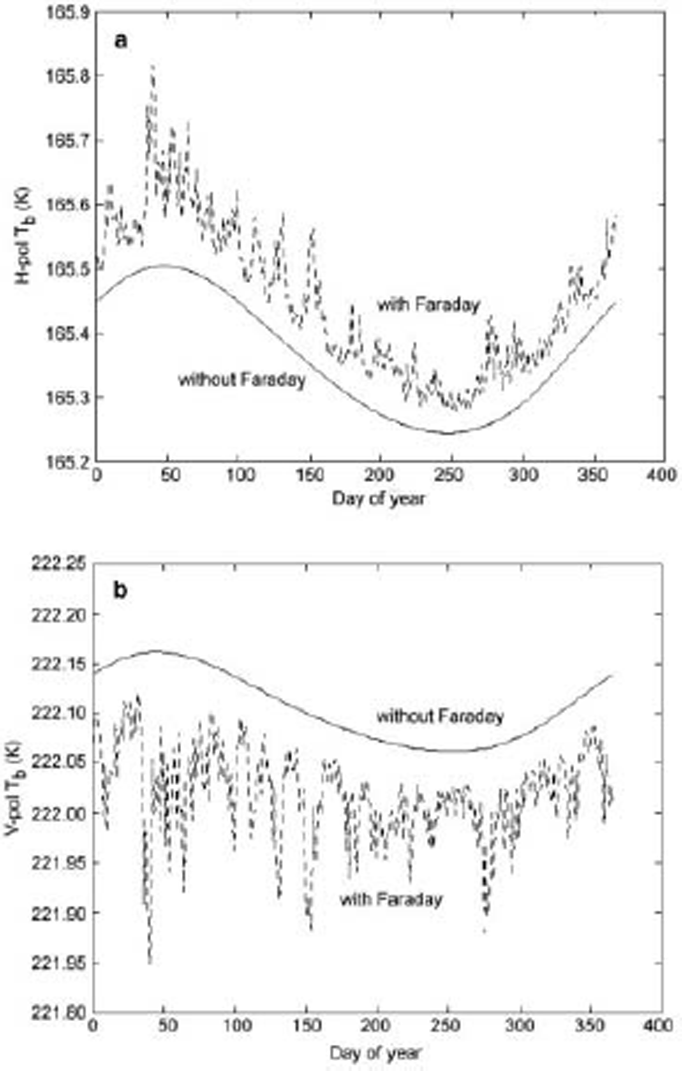
Fig. 5. Simulated temporal variations of the L-band H-pol (a) and V-pol (b) brightness temperature T _b over Dome C, with (dashed line) and without (solid line) the inclusion of Faraday rotation effects within the SMOS field of view at an incidence angle of 45˚.

Direct measurements of the electron content at high latitudes do exist. Incoherent scatter radar has been demonstrated to be an effective ground-based technique for the study of the ionosphere. For example, the EISCAT (European Incoherent SCATter) Scientific Association is an international research organization operating three incoherent scatter radar systems, at 931, 224 and 500MHz, two of which are situated near Tromsø, Norway, and one of which is near Longyearbyen, Svalbard, at 78˚N (see http://www.eiscat.no/). The latitudes of these observing stations are comparable to that of Dome C, so for the purpose of this discussion the observed variability is assumed to be comparable to that experienced at Dome C in the Southern Hemisphere.

Example measurements were obtained by EISCAT for several consecutive days in November 1989. The radar measures a profile of electron density, and the TEC is derived from the integration of the radar data between 90 and 500 km. To obtain a TEC value equivalent to that seen at nadir at SMOS satellite altitude (757 km), this value has been multiplied by a factor of 1.33 (Reference Lilensten and BlellyLilensten and Blelly, 2002).

Large cyclical variations of the electron-content-induced error are evident in Figure 6 due to the diurnal effect, with peaks of up to 3 K occurring shortly after 1200 h. The solar flux and the zenith angle control the amplitude of these variations. Notably, during the assumed ‘quiet’ period of the day (i.e. night and early morning) the ionosphere may still be subject to perturbations as a result of auroral precipitations. During the first period between 20 and 30 h local time, TEC can exhibit variations of a few TEC units (1016em^–2) over short time periods, with corresponding peak errors of 0.5 K.

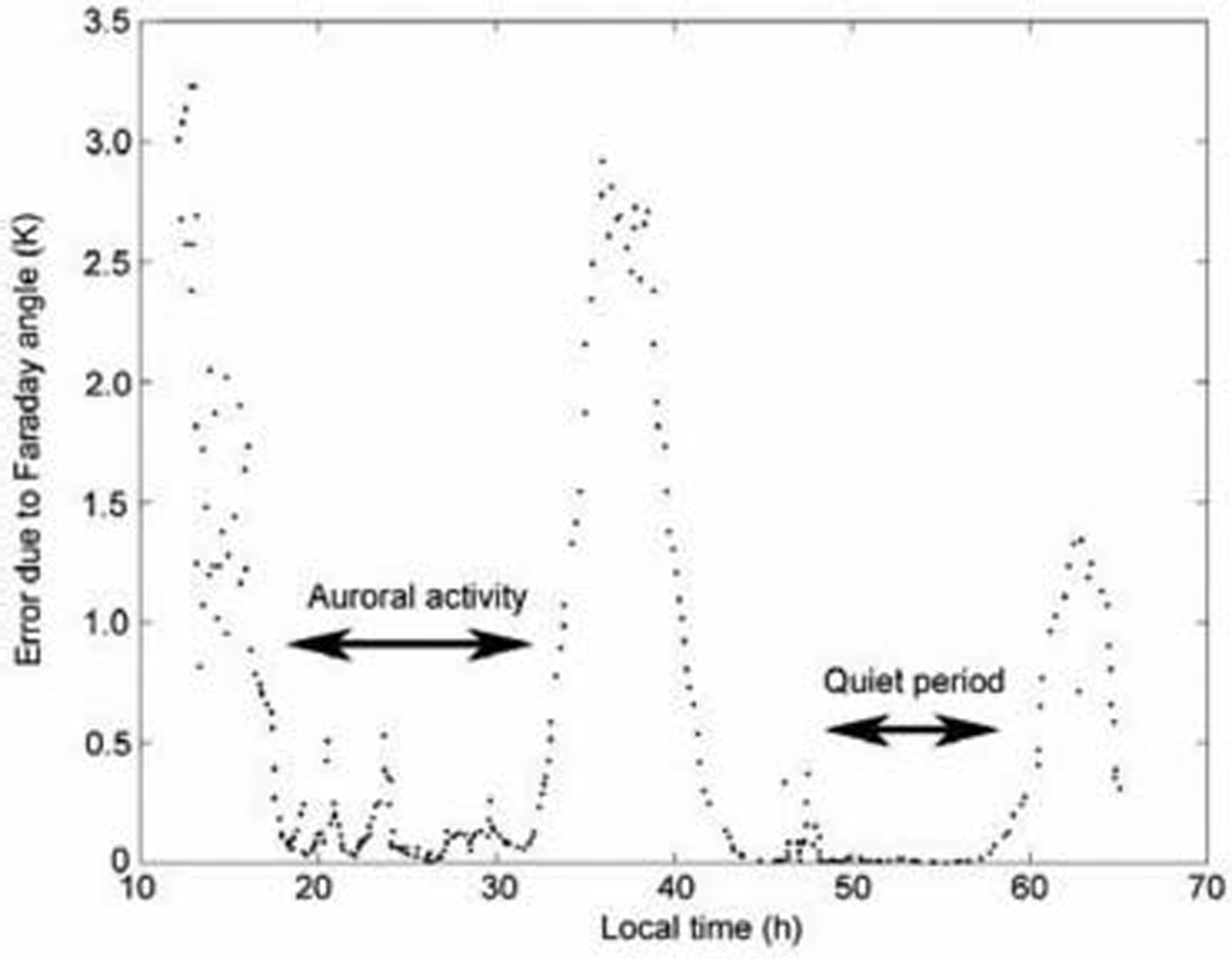
Fig. 6. Magnitude of the error in linear polarized brightness temperature caused by the inclusion of auroral Faraday rotation effects at an incidence angle of 45˚ during active and quiet periods of auroral activity over the period 14–16 November 1989.

Accurate calibration of SMOS will therefore require careful treatment of ionospheric effects. A strategy for dealing with ionospheric perturbations may be sought by using the amplitude of the first Stokes parameter I ₀ which represents the sum of the squared brightness temperatures at linear V- and H- polarization (i.e. I ₀ = |E ^V|² + |E _H|²). As such, I ₀ is insensitive to Faraday rotation. Since the SMOS radiometer will measure the full Stokes vector, future work will focus on calibration-error mitigation and correction strategies. Within the 11 year solar cycle, 1989 was a year of strong solar activity; TEC levels are expected to be lower during SMOS mission operations.

Conclusions

Historical microwave brightness temperatures acquired from SMMR and SSM/I confirm the long-term stability of the annual radiometric cycle in the region of Dome C on the East Antarctic plateau. Results indicate that the amplitude of the seasonal cycle diminishes with decreasing frequency (increasing wavelength) because a greater depth of the ice sheet contributes to microwave emission and the brightness temperature recorded by satellites at longer wavelengths. At depths below around 10m the annual variation in bulk physical temperature is negligible. Consequently there is only a small seasonal amplitude in brightness temperature at C-band (around 6 GHz) due to the greater penetration at this wavelength.

Multi-frequency electromagnetic model simulations using the MIMESI-MC model confirm that the depth from which thermal microwave emission originates is regulated by the vertical profile in temperature, and snow physical characteristics. L-band brightness temperature is extremely stable and controlled by the temperature at several hundred metres depth, and the seasonal amplitude in T _b is likely <0.1 K.

A combination of simulations and incoherent scatter radar data indicates that the ionosphere is subject to strong high-frequency fluctuations. These high-frequency spurious effects may be superimposed upon the more typical diurnal variations of the electron content at these high latitudes. As a consequence, it is difficult to argue that the brightness-temperature measurement error caused by Faraday rotation will remain constant. Nonetheless, results indicate that random variability is minimized at certain local times. Since the high-latitude location of Dome C facilitates a large number of potential acquisitions over the target site each day, it should be possible to avoid periods of auroral precipitation during which time the less predictable contribution to errors can be minimized.

Plans exist for conducting in situ L-, C- and Ka/Ku-band radiometer measurements and snow-pit sampling at Concordia Station, situated on Dome C, during the austral summer of 2004/05. Direct measurements at L-band will help model validation and provide a source of information with which to further characterize the azimuth- and incidence-angle diversity in spectral radiometric signatures. So far, the effects of temporal variability in surface and layer interface roughness have been neglected, along with the effects of azimuthal anisotropy previously observed in passive microwave data (Reference Long and DrinkwaterLong and Drinkwater, 2000). These in situ data will further help to establish scientific interest in use of the Dome C site as a multi-mission calibration and validation site. Current and future satellite instruments/missions that could potentially benefit from use of Dome C as an external calibration site are: the Microwave Radiometer (MWR) on Envisat; the Advanced Microwave Scanning Radiometer (AMSR) on Aqua/ADEOS-II; the Advanced Scatterometer (ASCAT) on METOP; CryoSat; and SMOS and Aquarius.