

1. Introduction
Results from the Antarctic have established that tabular icebergs move and bend in response to the ocean wave field (Foldvik and others 1980, Kristensen and others 1981, 1982). Furthermore, the icebergs act as low pass filters and respond only to the long-period part of the ocean wave spectrum. Clear indications of resonance are seen in the field data for all the characteristic bodily motions (heave, roll, pitch, surge and sway), and resonant peaks also occur in the measured surface strain data. Most of the wave energy in power spectra calculated from the measured records is concentrated at periods between 5 and 40 s, depending on the structure and shape of the iceberg, and on the forcing wave field. However, resonance in roll has also been observed at periods as high as 100 s (Kristensen and others 1982).
Research into the sea-keeping characteristics of tabular icebergs is relatively new and very little work is found in the literature. Expressions given in some earlier papers for the rolling response of icebergs are either inaccurate (Reference SchwerdtfegerSchwerdtfeger 1980) or neglect important factors such as the position of the centre of roll or fluid dynamical contributions (Foldvik and others 1980). Moreover, no earlier work on iceberg modelling has included the hydrodynamical effects of added inertia and linear damping; yet a comparison with field data reveals that simpler expressions cannot consistently provide a reliable picture of the motions of an iceberg (Kristensen and others 1982).
The ultimate aim of modelling the motions and flexural bending of tabular icebergs is to understand the break-up process more completely. There is no doubt that ocean waves can induce large icebergs to fracture by a complex fatigue process which slowly weakens the berg as it drifts northward. Resonance effects are also suspected of being important in the ultimate demise of the iceberg. Figure 1 shows an Antarctic tabular iceberg, with a heavily crevassed surface, photographed near the South Sandwich Islands.
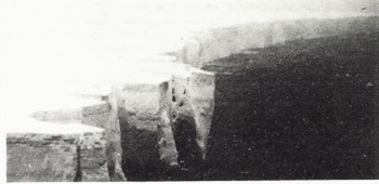
Fig. 1. Photograph of badly crevassed iceberg near the South Sandwich Islands.
The origin of the crevasses is unknown, but whether they were created by wave-induced bending, or by temporary grounding of the berg in shallow water, or by deformation before the berg calved, is unimportant when one considers the considerable influence that these features will have on local stress concentration. Clearly, modelling of icebergs with such complicated mechanical response is difficult, and requires a knowledge of the behaviour of the iceberg at sea. Although detailed conclusions about flexure and fracture cannot be drawn from the present paper, as we stop short of a complete flexural study, the modelling of the rigid body motions themselves can uncover some interesting characteristics of tabular icebergs at sea.
Modelling of the wave-induced motions of tabular icebergs falls naturally into two parts: firstly, the rigid body response, including the motions of heave, roll, pitch, sway and yaw, and the hydrodynamically induced pressure beneath the berg, is calculated; then, secondly the computed pressure along the wetted surface is used to provide the necessary forcing to model the cyclic flexure of the berg due to passing ocean waves. The method assumes that the flexural amplitudes are small compared to the amplitudes due to rigid body motion, and that no interaction occurs between the two types of motion. Results from the first phase of the analysis only will be discussed in this study.
2. A Two-Dimensional Model of Tabular Icebergs in Ocean Waves
The technique on which this paper is based was originally developed by Reference FrankFrank (1967) and Bedel and Lee (1971), and has been adapted to model ice floes by Squire (1981, 1983). In the present paper we shall mention only briefly the main points of the method, together with necessary modifications for modelling of tabular icebergs. The method is entirely numerical and uses a polygonal representation of the underwater contour of the iceberg. The basic assumptions are: (a) the model is linear and two-dimensional, (b) the iceberg is semi-submerged and in neutral buoyancy, (c) no drift occurs, i.e. oscillatory motions only, and (d) the depth of the water is infinite and there is no current.
There are several reasons for choosing to model icebergs with a two-dimensional model. Firstly, a three-dimensional model makes computing particularly difficult and expensive. Secondly, our aim is to model real icebergs and to reproduce results from in situ measurements. Since our input forcing (records from the Waverider buoy) is not directional, we feel that the gain of using a three-dimensional model will largely be lost. Throughout the modelling we have kept a careful control on our results by comnaring them with field data.
It is well known that a body moving in a fluid will induce frequency-dependent forces which oppose the motion, and will create and sustain outgoing surface waves. Two hydrodynamical effects are associated with the resistance of the fluid to the motions of the floating body; the first is the added inertia and the second may be interpreted as damping. In our model, damping is synonymous with surface wave generation since the equations of motion have been linearized. Viscous damping, a non-linear effect which is important for roll and pitch, is neglected in this study, although it may be included at a later stage. For heave, the equation of motion is given by
where z(t), z and z are, respectively, the displacement, velocity and acceleration of vertical motion, M is the mass of the iceberg, a is its added mass, b is the linear damping coefficient, and F is the vertical wave-exciting force. C, the restoring coefficient, is given by C=pgB, where p is the water density, g is the acceleration due to gravity, and B is the length of the iceberg. Similar equations may be written for the other translatory and rotatory motions. The problem in solving the apparently simple equations of motion lies in evaluating the added inertia and the damping coefficients, and in finding the coupling between successive equations. Further details of the theoretical background to the model, as well as details of the effect of neglecting important terms, may be found in Reference LeeLee (1976).
The input and output parameters in the model are as follows. Input: contour geometry of the submerged part of the body, radius of gyration, position of the centre of roll, and the period and direction of incoming ocean waves. Output: rigid body motion amplitudes and phases, added mass (inertia) and damping for the rigid body motions, pressure fields resulting from different rigid body motions, and the total pressure field on the body contour. Motion amplitudes are scaled to an incoming ocean wave of 1 m in all the figures presented. To convert to the motions actually experienced by a real iceberg it is necessary to multiply results by the scaling factor, viz. the observed ocean wave amplitudes or RMS amplitudes derived from power spectra. The model is quite general and allows the bodily response to be calculated at any position on the iceberg. However, for simplicity we shall present results for the centre of the surface of the berg only, where most field data are collected. Furthermore, we shall not discuss phase in the present study. Figure 2(a) shows definitions of geometry and some terms used in describing the motion of icebergs.

Fig. 2. Iceberg Geometry (a) and Some Parameters Used in The Model 1Ing (b).
The geometric shape and structure of the tabular icebergs play an important role in the analysis, and the model is naturally very sensitive to changes in radius of gyration and the axis about which the berg rolls (centre of roll). This is shown in Figure 3, where amplitudes of motion at different periods of beam-on waves are presented for a homogeneous iceberg with horizontal dimensions of 1 000 × 800 m, and a thickness of 250 m, icebergs of this shape and size being common in the Antarctic (Reference NazarovNazarov 1962). The sway, heave and roll motions shown illustrate the effect of a 10% change in the radius of gyration and the position of the centre of roll. As expected, the heave response is unchanged, but the changes seen in sway and roll are large.

Fig. 3. Sway, heave and roll motions for standard iceberg (solid line), iceberg with 10% shift in centre of roll (dashed), and iceberg with 10% change in radius of gyration (dotted).
Studies of the density structure of tabular icebergs have not penetrated deeper than the surface layers, so it is impossible to calculate the radius of gyration directly. However, the density structure of the icebergs can be inferred by radio echo profiles of thickness and freeboard, and from density profiles measured in ice-shelf cores. The density profiles used in the modelling are shown in Figure 2(b). The centre of roll is taken to be fixed at the centroid of the waterplane. Although this is not strictly accurate, because the position of the centre of roll is a complex function of the amplitude and period of the incoming wave and the mass distribution and shape of the iceberg, we consider it to be a good approximation. For a perfectly tabular iceberg it is easy to find the vertical position of the centre of roll as a function of the density profile, since this is essentially the same as finding the freeboard. Thus, the calculation of the radius of gyration and the position of the centre of roll should be seen as interdependent.
In Figure 4 we show graphs of amplitudes of motion for several different freeboard-to-draft ratios, i.e. different density profiles, but with the same geometry. Although there are some differences in the motion amplitudes for the ratios corresponding to different density profiles, these are not significantly large. We therefore conclude that if the correct freeboard-to-draft ratios are established for tabular icebergs, satisfactory radii of gyration and centres of roll can be found. The density profile of the solid curve in Figure 4 corresponds best with the field data on iceberg geometry, and we shall use it consistently in the following discussion.
Fig. 4. Sway, heave and roll motions for various density profiles.
3. Modelling of Perfectly Tabular Icebergs
The rigid body motions of a standard-sized iceberg (we have chosen the geometry used in section 2) are shown in Figure 5(a) where sway, heave and roll amplitudes are plotted as functions of incident ocean wave period. All the curves have clear resonant peaks: sway at 37 s, roll at 48 s, and heave at 52 s. As expected, both the sway and heave curves tend to perfect response at very large periods (i.e. they follow the motion of the wave), while the rolling motion of the iceberg is negligible for very long waves. The sway motion shows a minimum around 52 s. This behaviour in sway is well documented in the literature and we shall not discuss it further (Reference VugtsVugts 1968).
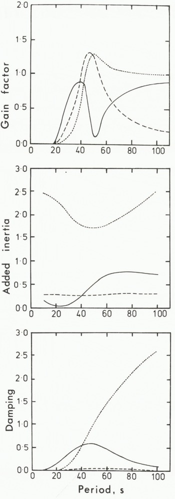
Fig. 5. Motions and characteristics of standard iceberg: (a) gain factor, (b) added inertia, and (c) damping. Sway (solid line), heave (dotted) and roll (dashed). The added masses for sway and heave have been scaled by pSa where Sa is the underwater sectional area, and the added inertia for roll by
Figures 5(b) and (c) clearly demonstrate the importance of including added inertia and damping in the model. Their variation for roll with incident wave period is small, but the same parameters for heave and sway are strongly dependent on period. A simpler modelling approach with added inertia and damping neglected or represented by constants would therefore yield unacceptable results. Damping is directly related to the outgoing waves created by the motions of the iceberg. Figure 5(c) therefore illustrates that the wave-making potential of the standard iceberg is largest in the heave mode and at relatively long wave periods. Damping for sway is largest at mid-periods and is small for short and long waves, while roll damping is always small.
The next step in our modelling is to study the effects of varying geometry. For all such variations the same density profile has been used, but new values of radius of gyration and centre of roll have been calculated as required. Gain factors for sway, heave and roll are presented in Figure 6 for three icebergs of varying length. All three motion response modes show marked differences as the beam of the iceberg decreases. Sway amplitudes are small for incident wave periods of less than 30 s and quickly approach the incident wave amplitude in magnitude above periods of 60 s. The longer berg shows a large sway response at periods between 20 and 80 s but the usual minimum occurs at a much greater period than the standard berg and its short counterpart, where the minimum is not so marked. The main effect of increasing the length of the iceberg on the other bodily motions is to decrease the severity of resonance in heave, and to increase it in roll. Not unexpectedly, the period of resonance increases with length.
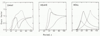
Fig. 6. Sway, heave and roll motions for icebergs of different lengths. Iceberg of length of 1 000 m is represented by solid line, 4
Amplitudes of motion for icebergs of varying thickness are shown in Figure 7, In sway, the first peak is moved only slightly with increased thickness, but its amplitude becomes significantly smaller as the iceberg thickens. This is also the case for the response to roll. The resonant peak in the heave motion is markedly larger for the thicker iceberg.
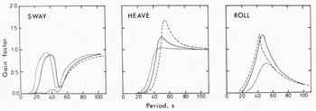
Fig. 7. Sway, heave and roll motions for icebergs of different thickness. A thickness of 250 m is drawn as solid line, 400 m by dashed line, and 150 m by dotted line.
pSa,B2/4. The scaling for damping is the same as for added inertia but has also been divided by the circular frequency of the wave.
Since we are using a two-dimensional model, the variation of width will not affect the results for incident beam waves. We shall therefore consider the amplitudes of motion generated by waves incident at an angle of 135° (bow-quartering waves). The results are presented in Figure 8 and it is interesting to note that, while the period at which resonance occurs does not vary much with width, the response amplitudes of our standard iceberg are larger than those for both the smaller and larger icebergs.
Finally we show some examples of the total forcing pressure field along the underside of tabular icebergs. We have chosen an incident wave period of 15 s, and in Figure 9(a) we have compared the pressure variations for a thick and a thin iceberg with those for our standard iceberg. In Figure 9(b) the same comparison is made for a long and a short iceberg. It is evident that the pressure gradient along the bottom of the thinner icebergs is significantly larger, and this is also the case for longer icebergs. Since flexural surface strain will increase with pressure gradient along the underside of the iceberg, field observations indicating that long, thin icebergs break up faster should be confirmed by these preliminary results. However, the full flexural solution is obviously necessary to obtain reliable conclusions.
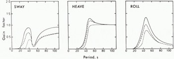
Fig. 8. Sway, heave and roll motions for bow-quartering waves and varying widths. Solid line represents iceberg of width of 800 m, dotted represents 2 000 m, and dashed represents 400 m.
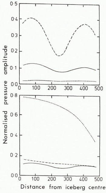
Fig. 9. Normalized pressure experienced at underside of iceberg: (a) for varying thickness and (b) for varying length. The horizontal axis in Figure 4(b) is scaled by 4 for the long iceberg and 0.4 for the short iceberg for convenience. Pressures are normalized by a factor pg.
4. Conclusions
Because of logistic difficulties and costs, there have been few field studies of Antarctic tabular icebergs. As a result, little material is available for comparison with modelling results. A traditional view has been that no energy is to be found in the ocean wave spectrum at very long periods, and that the resonant response of tabular icebergs would therefore rarely be exited. However, it has been shown on two recent field trips that very long period resonance (above 40 s) can be found in all the rigid body motions of icebergs of different geometries (Kristensen and others 1981, 1982). Since existing techniques of wave measurement rely on the use of accelerometers, or more recently on radar altimetric data collected by satellite (Mognard and others 1982), it is possible that wave energy at long periods has hitherto remained undetected. It is known, however, that wave packets on the scale of the sea’s modulation envelope are present and could provide energy at these very long periods of oscillation. The first indications from iceberg measurements is that such long period events are sustained over a long time scale rather than being a single event which would rapidly be damped out, but further field research is necessary in order to make detailed conclusions on the nature of these ocean wave phenomena.
The results from our modelling so far confirm results from the two field trips described in Kristensen and others (1981, 1982) and can be summarized as follows: (i) for an iceberg with one horizontal dimension much larger than the other, the sway response is dependent on the direction of the incident waves, and is smallest for thicker icebergs, (ii) for the same iceberg, the heave response is smaller than that for the squarish, medium-sized iceberg, and becomes more peaked as thickness increases, and (iii) the largest iceberg has the largest roll response, and the effect of changing the length of one horizontal dimension compared to the other is to increase the period at which resonance occurs.
The modelling presented in this paper makes it possible to calculate the forcing pressure fields at the bottom and sides of tabular icebergs as a function of iceberg geometry and structure as well as incident wave periods and amplitudes. Thus the results from the model form a foundation on which to model further the flexural bending of tabular icebergs.
4. Conclusions
Because of logistic difficulties and costs, there have been few field studies of Antarctic tabular icebergs. As a result, little material is available for comparison with modelling results, A traditional view has been that no energy is to be found in the ocean wave spectrum at very long periods, and that the resonant response of tabular icebergs would therefore rarely be exited. However, it has been shown on two recent field trips that very long period resonance (above 40 s) can be found in all the rigid body motions of icebergs of different geometries (Kristensen and others 1981, 1982). Since existing techniques of wave measurement rely on the use of accelerometers, or more recently on radar altimetric data collected by satellite (Mognard and others 1982), it is possible that wave energy at long periods has hitherto remained undetected. It is known, however, that wave packets on the scale of the sea’s modulation envelope are present and could provide energy at these very long periods of oscillation. The first indications from iceberg measurements is that such long period events are sustained over a long time scale rather than being a single event which would rapidly be damped out, but further field research is necessary in order to make detailed conclusions on the nature of these ocean wave pnenomena.
The results from our modelling so far confirm results from the two field trips described in Kristensen and others (1981, 1982) and can be summarized as follows: (i) for an iceberg with one horizontal dimension much larger than the other, the sway response is dependent on the direction of the incident waves, and is smallest for thicker icebergs, (ii) for the same iceberg, the heave response is smaller than that for the squarish, medium-sized iceberg, and becomes more peaked as thickness increases, and (iii) the largest iceberg has the largest roll response, and the effect of changing the length of one horizontal dimension compared to the other is to increase the period at which resonance occurs.
The modelling presented in this paper makes it possible to calculate the forcing pressure fields at the bottom and sides of tabular icebergs as a function of iceberg geometry and structure as well as incident wave periods and amplitudes. Thus the results from the model form a foundation on which to model further the flexural bending of tabular icebergs.
Acknowledgements
The authors gratefully acknowledge the help of Professor Choung Lee of the David w Taylor Naval Ship Research and Development Center, Bethesda, Maryland, USA, who originally developed the model and brought it to Cambridge. We also thank Rob Massom for drawing the diagrams. We are grateful to the British Petroleum Co Ltd for financial support, and to the British Council who supported MK as a research student.


