Introduction

In Japan, especially in the region facing the Sea of Japan, we have plenty of snowfall in winter. Heavy snowfalls cause serious disasters, such as snow avalanches, house collapses under weight of snow, and traffic jams. On the other hand, snow constitutes an appreciable percentage of the total water resource in the snowy region. To protect against possible snowfall damages, and to make an efficient use of snow, it is necessary to forecast and estimate snowfall distribution.

In winter the northwesterly monsoon is greatly modified by its passage over the Sea of Japan and brings a characteristic weather to the downstream region. Snowfall on the windward side of Japan is undoubtedly related to the moisture and heat supplies resulting from air-sea interaction (Reference Matsumoto and NinomiyaMatsumoto and Ninomiya, 1966; Reference Matsumoto, Ninomiya and AkiyamaMatsumoto and others, 1968; Reference NinomiyaNinomiya, 1972), though it is difficult to observe these values directly using ships or aircraft during the strong winter monsoon. Clouds are the visible manifestation of convective activities which redistribute the heat and moisture in the free atmosphere, release the sensible heat, convert potential energy into kinetic energy and serve as a reservoir of water themselves. The observation of clouds, which may be carried out rather easily using satellite remote sensing, is useful for understanding the physical processes in the atmosphere.

There are two types of clouds which cause heavy snowfall in Japan: mesoscale vortex-like clouds and streak-like clouds. The former cause heavy snowfall on the coastal plain and the latter on the mountainous region. The small-scale lows develop in the polar air streams around Japan. Radar and satellite observations indicate that some lows are accompanied by high spiral echo bands and cause intense precipitation (Reference MiyazawaMiyazawa, 1967; Reference Asai and MiuraAsai and Miura, 1981; Reference NinomiyaNinomiya, 1989). The aligned cumulus rows referred to as streak-like clouds usually appear under the strong winter monsoon over the Sea of Japan and sometimes continue for several days; there are good opportunities for observating them using Earth-orbiting satellites. The cumulus-scale convection is regarded as a very important eddy motion in the large-scale atmospheric process because the heat and moisture, which are supplied from the sea to the air, are redistributed in the free atmosphere mainly by this cumulus convection (Reference Matsumoto and NinomiyaMatsumoto and Ninomiya, 1966; Reference Matsumoto, Ninomiya and AkiyamaMatsumoto and others, 1968; Reference NinomiyaNinomiya, 1968). In this paper, the characteristics of streak-like cloud, such as the three-dimensional structure and the distributions of column water vapor and cloud liquid contents, are investigated using the data of Landsat and MOS-1.

Three-Dimensional Structure of Streak-Like Cloud

Detailed information on the three-dimensional shape of clouds has been derived from the Landsat Thematic Mapper (TM) image on 9 January 1987. The spatial resolution of the Landsat TM is 30 m in the visible and near-infrared bands and 120 m in the thermal infrared band. The study area is located at a distance 250 km east of Vladivostok and its size is about 185 km square. As shown in Figure 1, which is the visible-band image of the study area, there are several aligned cumulus rows and the activity differs with each row. Seven rows are selected and several 10 km square sub-areas along each row, which are shown in Figure 1, are investigated in detail.

Fig. 1. Visible image of the Landsat TM of the study area on 9 January 1987. Open squares show sub-areas selected for detail investigation.

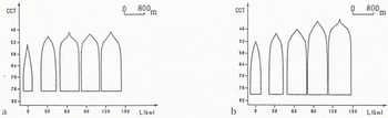
In each sub-area, cloud region is derived from the visible image using the method of edge enhancement and is sliced using the thermal infrared band, i.e. the higher parts of clouds correspond to the pixels of the lower brightness temperature. Then clouds are expressed by the contour-line map of the computer-compatible tape (CCT) counts of the thermal infrared band (Fig. 2) and the three-dimensional perspective view (Fig. 3), which show the convective cells.

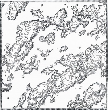
Fig. 2. Contour-line map of sub-area A2, using CCT counts of the thermal infrared band of Landsat.

Fig. 3. Three-dimensional perspective view of sub-area A5, using CCT counts of the thermal infrared band of Landsat.

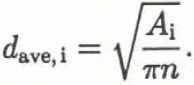
In order to identify the three-dimensional structure of convective cells in a sub-area, that average diameter of cells, d _ave,i, is calculated at a given CCT count level of the thermal infrared, C _i, as follows.

1. The number of peaks of clouds in a sub-area, n, is counted using the contour-line map and several three-dimensional perspective views.

2. It is assumed that the number of peaks corresponds to the number of convective cells in the sub-area.

3. The total cloud surface area at less than C _i namely A _i, is measured using digital image-processing software.

4. Representing sections of these cells to be circular gives

   (1)

   

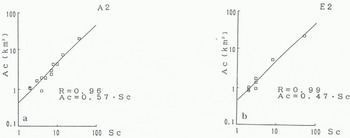
The CCT count of the cloud base is identified as the threshold value chosen to separate clouds from sea surfaces in the sub-area. Then the average vertical sections of convective cells in each sub-area along each row are obtained as shown in Figure 4. In this figure, the distance from the starting point of a streak-like cloud is taken as the abscissa and the CCT count of the thermal infrared band as the ordinate. Figure 4 shows that a convective cell rapidly changes shape from a cone to a column and its size becomes constant both horizontally and vertically along each row. The relationship between the cloud area and the number of the convective cells within the cloud in each sub-area is regressed by the linear function as shown in Figure 5, in which the intercept of the straight line corresponds to the average area of convective cells. Table 1 shows that convective cells have a uniform value of average area and the average diameter is about 800 m over the study area. Therefore, the aligned cumulus row consists of a large number of uniform convective cells and its activity depends on the concentration of cells, as shown schematically in Figure 6.

Fig. 4. Average vertical sections of the convective cells along the row. a, sub-area A (see Fig. 1); b, sub-area E (see Fig. 1).

Fig. 5. Relationship between the cloud area and the number of the convective cells within the sub-area, a, sub-area A2 (see Fig. 1); b, sub-area E2 (see Fig. 1).

Table 1. Average area (km²) of a convective cell in each sub-area

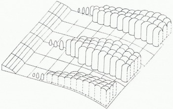
Fig. 6. Schematic expression of streak-like clouds.

Distribution of Column Water Vapor and Cloud Liquid Contents

Microwave remote-sensing techniques can be employed to monitor atmospheric parameters and weather con-ditions. Absorption resonances due to water vapor at 22.2 GHz and the low-attenuation “atmospheric window” at 35 GHz can be used to determine column water vapor and cloud liquid contents through radiometric measurements near the absorption maximum and the attenuation minimum. Grody (Reference Grody1976) presented an equation which makes it possible, through two frequency measurements of brightness temperature, to determine the total water vapor, W, in g cm⁻², and the total liquid water content, Q, in kg m⁻², given a reasonable estimate of surface temperature, T_B, emissivity, ε_s (v), and mean cloud temperature, T _cl, for a non-scattering atmosphere in local thermodynamic equilibrium. It is given as follows:

(2)

where Τ _B is the nadir brightness temperature at frequency v in GHz. W ₀ (v) and Q ₀ (V) are the column water vapor and liquid water corresponding to the unit absorption coefficients, respectively. The latter is expressed using T _cl, as follows:

(3)

To evaluate these, two sensor systems aboard MOS-1 are used: the Microwave Scanning Radiometer (MSR) and the Visible and Thermal Infrared Radiometer (VTIR). The MSR observes the Earth at 23.8 GHz and 31.4GHz. These frequencies are optimal for separately retrieving water vapor and cloud liquid contents in the atmosphere using Equation (2). Two thermal infrared bands of the VTIR are used for estimating the surface temperature and the mean cloud temperature. Figure 7 shows the thermal infrared image of the VTIR over the Sea of Japan on 10 January 1988. There are two typical cloud patterns, the longitudinal mode and the transverse mode, which usually appear under the winter monsoon. The study area is limited by the observational swath of the MSR, which is smaller than the VTIR swath. Figure 8 shows a part of Figure 7 which is extracted to correspond to the MSR swath for this study. Ten sub-areas along the leeward in each cloud mode are selected for comparison of the distributions of water vapor and cloud liquid contents.

Fig. 7. Thermal infrared image of the MOS-1 VTIR of the study area. L is the longitudinal mode and Τ is the transverse mode.

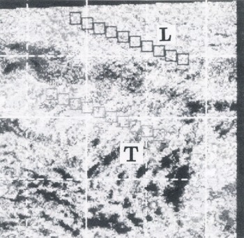
Fig. 8. Part of the VTIR image extracted to correspond to the MSR swath. Small boxes show sub-areas selected for detailed investigation.

The analyzed result is shown in Figure 9. Figure 9a shows that the water-vapor content is uniform over the study area and its variation along the leeward is very small. On the contrary, in the longitudinal mode both the cloud liquid content and its variation are larger than in the transverse mode, as shown in Figure 9b.

Fig. 9. Distribution of column water vapor and cloud liquid contents (□,L mode; , Τ○ mode). a, water vapor content; b, cloud liquid content.

Conclusions

Two methods are presented for analyzing cloud development under the winter monsoon using satellite data. The results of applications of these methods to a case study follows.

1. Using Landsat TM data, the three-dimensional shape of aligned cumulus rows have been identified for an initial case as follows:

• a. convective cell rapidly changes shape from a cone to a column;

• b. the rows are composed of a number of convective cells of nearly the same horizontal scale;

• c. the strength of convection of a row is evidenced by the concentration of convective cells.

1. Data on water vapor and cloud liquid-water contents over the Sea of Japan have been retrieved for a different case, but under similar airflow conditions, using two microwave bands of the MSR (23.8 GHz and 31.4 GHz) and two thermal infrared bands of the VTIR and applying the radiative transfer equations. The results show that water-vapor content was uniform over the sea, while cloud liquid content depended on the modes of cumulus rows under strong winter monsoon.

In order to form general conclusions many cases will be analyzed.