


1. Introduction
In response to global temperature increase, glaciers located in Alaska, as in almost every region of the world, have shown a strong retreat since their Little Ice Age maximum extent, with a more pronounced acceleration during the last decades of the 20th century (Reference MolniaMolnia, 2007; Reference Zemp, Roer, Kääb, Hoelzle, Paul and HaeberliWGMS, 2008). To better understand and model the response of glaciers to climate change, global inventories in a digital format are required (e.g. Reference BeedleBeedle and others, 2008; Radic ć and Hock, 2010). In the case of Alaska, the main purpose of an inventory is better quantification of the glacier melt contribution to global sea-level rise (e.g. Reference Kaser, Cogley, Dyurgerov, Meier and OhmuraKaser and others, 2006; Reference Berthier, Schiefer, Clarke, Menounos and RémyBerthier and others, 2010), as well as the modeling of future changes in water resources (Reference Zhang, Bhatt, Tangborn and LingleZhang and others, 2007).
As a contribution to the European Space Agency (ESA) GlobGlacier project (Paul and others, 2009), this study focuses on the generation of accurate glacier inventory data from nine Landsat Thematic Mapper (TM) scenes acquired between 2005 and 2009 for a region with previously poor coverage (from the Chugach to the Chigmit Mountains) in both the World Glacier Inventory (WGI; Reference Haeberli, Boösch, Scherler, Østrem and WallénWGMS, 1989) and the Global Land Ice Measurements from Space (GLIMS) glacier database (Reference RaupRaup and others, 2007). In a previous study, Reference Manley, Williams and FerrignoManley (2008) stressed the importance of putting effort into creating a glacier inventory from already available data compiled by the US Geological Survey (USGS) in the 1950s for the eastern part of the Alaska Range. We have thus decided to use the digitally available version of this earlier glacier survey to assess mean decadal changes in glacier size for a subset of selected glaciers. The new dataset is available through the GLIMS website (http://www.glims.org).
2. Study Region and Input Data
2.1. Study region
The study region is situated around the Gulf of Alaska (Fig. 1), with glaciers ranging in altitude from sea level up to 4000ma.s.l. To provide a more regionalized assessment of glacier inventory data, the region was divided into seven subregions: (1) Tordrillo Mountains, (2) Chigmit Mountains, (3) Fourpeaked Mountain, (4 and 5) south and north Kenai Mountains, (6) Chugach Mountains and (7) Talkeetna Mountains. While the Tordrillo Mountains are situated in the southern part of the Alaska Range, the Chigmit Mountains and Fourpeaked Mountain are also considered to belong to the Aleutian Range and extend south of the Tordrillo Mountains to Kamishak Bay. There are several thousand glaciers in these mountain ranges, representing a large variety of glacier types from small cirques to large valley glaciers with multiple basins (Reference Denton, Field and FieldDenton and Field, 1975). Several of the glaciers are classified as surge-type (e.g. Hayes and Harpoon Glaciers) and some of them cover volcanoes (e.g. Crater Glacier on Mount Spurr (3374ma.s.l.)).
The Kenai Mountains are located on the Kenai Peninsula between Cook Inlet and the Gulf of Alaska. The maximum elevation of glaciers here is ~2000ma.s.l., and the three main ice masses are the Sargent and Harding ice fields and an unnamed ice cap. The part of the Chugach Mountains considered here is bounded on the east by the Copper River and on the west by the Knik Arm. Together, these mountain ranges contain about one-third of the glacierized area of Alaska (Reference Post and MeierPost and Meier, 1980). Many large glaciers (e.g. Harvard, Yale, Columbia, Shoup and Valdez glaciers) are of tidewater type and drain into northern Prince William Sound. In the west, until 1966, Knik Glacier dammed the outflow from Lake George, resulting in nearly annual glacier-outburst floods (Reference Post and MayoPost and Mayo, 1971). The Talkeetna Mountains are the final region surveyed in this study. They are located north of the Matanuska River and north of the Chugach Mountains. Many peaks are higher than 2000m a.s.l., with a maximum elevation of 2550ma.s.l. As the entire study region includes glaciers of all types, with highly variable elevation ranges and locations (from the coast to the interior), different climatic regimes and responses to climate change can be expected.
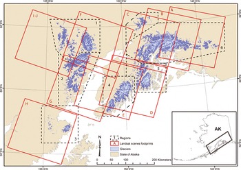
Fig. 1. Location map showing the footprint of the ten Landsat scenes originally analyzed in this study (red squares, where the red letters refer to the scene IDs). The sub-regions are delimited by dashed polygons, with the numbers referring to the IDs (see Tables 1 and 3), and glaciers are in light blue. The location of the study region in Alaska, USA, is shown in the inset.
In general, the study region experiences a predominantly maritime climate near the coast and a more continental climate further inland (e.g. http://climate.gi.alaska.edu). In the maritime region, mountain ranges act as a barrier for the westerlies, resulting in high amounts of annual precipitation along the coast of the Gulf of Alaska and frequent cloud cover. Clouds and frequent seasonal snowfields considerably decrease the number of useful satellite scenes in this region, so the inventory data refer to a 5 year period.
2.2. Input data
We analyzed all Landsat scenes from 1999 to 2009 that are freely available in the glovis.usgs.gov archive and processed to the standard terrain correction (level 1T). We selected ten of them covering our study region (Fig. 1; Table 1).
Table 1. List of the Landsat scenes used in the glacier inventory of western Alaska (source: http://glovis.usgs.gov). See Figure 1 for location of footprints; scene B was finally not used
Scene B (Enhanced TM Plus (ETM+) from 2002) was processed at the beginning of the study, though it had considerable amounts of seasonal snow hiding several glacier boundaries. When two scenes from 2009 (A and C) with much better snow conditions became available we decided to use these for the Chugach Mountains inventory.
For the western Alaska Range (scenes 72-17), we combined two scenes. The scene from 2005 (I) had much better snow conditions (particularly in the accumulation region), but the lower part of most low-lying glacier tongues was barely visible due to a dense layer of fog and/or smog from fire. The lower glacier parts were hence derived from the 2007 scene (J), in large part by manual digitization of the debris-covered tongues.
A digital elevation model (DEM) is required to calculate topographic glacier parameters (e.g. minimum, mean and maximum elevation, mean slope and mean aspect) and to perform hydrological analysis (watersheds) for determination of drainage divides to separate contiguous ice masses into individual glaciers (e.g. Reference Schiefer, Menounos and WheateSchiefer and others, 2008; Reference Bolch, Menounos and WheateBolch and others, 2010b). For the study region, we used the Advanced Spaceborne Thermal Emission and Reflection Radiometer (ASTER) global DEM (GDEM) and the USGS National Elevation Dataset (NED), both with a spatial resolution of 30 m, and for part of the region (south of 60˚N) the Shuttle Radar Topography Mission (SRTM) C-band DEM with resolutions of 100 (~30 m, SRTM-1) and 300 (~90 m, SRTM-3). The SRTM DEM is known for its accuracy, with a mean deviation from a reference dataset of ~3±15m (Reference Berry, Garlick and SmithBerry and others, 2007). However, it is less accurate in the rough terrain of high mountains, with typical problems of synthetic aperture radar (SAR)-derived DEMs (radar shadow, layover, foreshortening) causing data voids. We thus use the seamless SRTM DEM from the Consultative Group for International Agriculture Research (CGIAR), version 4, where these voids were filled with additional elevation information (http://srtm.csi.cgiar.org.) A study comparing SRTM-1 data with NED data in the USA revealed slightly higher accuracy of the SRTM-1 DEM in both the horizontal and vertical directions (Reference Smith and SandwellSmith and Sandwell, 2003).
The GDEM can be of good accuracy (Reference Hayakawa, Oguchi and LinHayakawa and others, 2008) but has inaccuracies mainly in regions of steep slopes and snow, due to missing contrast (Frey and Paul, unpublished information), and contains artifacts like local bumps and pits (depressions) which are typical for ASTER-derived DEMs (Reference KääbKääb and others, 2003; Reference ToutinToutin, 2008). However, these artifacts were not a problem for this study. Due to its northern limitation (60˚N), the SRTM DEM was available only for the southern part of the Kenai Peninsula, while the NED and the GDEM cover the entire region. Several tiles of both DEMs were downloaded, mosaicked and reprojected to Universal Transverse Mercator (UTM) zone 5 and bilinearly interpolated to 30m cell size. Hillshades were created for all three DEMs to better recognize artifacts. While the NED refers to the contour lines of the related topographic maps from the 1950s, the GDEM was created from all available scenes in the ASTER archive acquired between 1999 and 2007. Hence, the topography in the GDEM fits much better to the acquisition period of the Landsat data (Table 1) and was therefore used to calculate minimum glacier elevation.
The Digital Line Graph (DLG) dataset was utilized to calculate changes in glacier size (see section 3.3). This earlier glacier mapping was compiled by the USGS from the 1 : 63 360-scale 15″ topographic quadrangle maps. Because the DLG has been partly updated compared to the Digital Raster Graph (DRG), we only selected glaciers with a good coincidence of the outlines. The DRGs are a scan of the topographic maps that were created from vertical aerial photographs (1948–57) by stereophotogrammetric techniques. For glacier identification we used this DRG dataset from the USGS, the Geographic Names Information Service (GNIS) which is also available in a digital format http://geonames.usgs.gov/), the Alaska atlas and gazetteer (De-Lorme, 2004) and the recently published Alaska volume of the Satellite image atlas of glaciers of the world (Reference Williams and FerrignoWilliams and Ferrigno, 2008).
3. Methods
3.1. Glacier mapping
We use automated mapping as the basic method and only edit regions with wrong classification. The glacier-mapping technique is the well-established semi-automated band ratio method (TM3/TM5) with manual threshold selection (e.g. Reference Paul and KääbPaul and Kääb, 2005). This method is based on the specific spectral reflectance properties of snow and ice compared with other terrain. While reflectance of glacier ice and snow in band TM3 (red) is comparably high (with possible sensor saturation over fresh snow), it is very low in band TM5 (shortwave infrared (SWIR)). These spectral differences make the TM3/TM5 ratio very efficient at discriminating glaciers from other terrain. Further advantages of the technique are its reproducibility and consistency for an entire region, and its accuracy for clean to slightly dirty glacier ice (e.g. Reference AlbertAlbert, 2002; Reference Paul, Huggel, Kääb, Kellenberger and MaischPaul and others, 2003; Reference Andreassen, Paul, Kääb and HausbergAndreassen and others, 2008; Reference BolchBolch and others, 2010a). However, manual corrections are still needed, in particular for debris-covered ice, calving glacier termini and water surfaces. Applying an additional threshold in band TM1 (blue) improves the classification in cast shadow (Reference Paul and KääbPaul and Kääb, 2005). Before outlines are edited, a noise filter (low pass 3×3 median filter) is applied to remove isolated snowpatches and to close local gaps. The classified map is then converted to vector format and imported by Geographic Information System (GIS) software. In a post-processing step, the necessary corrections for clouds, shadow, debris cover and water bodies are applied. To facilitate the interpretation, false-color composite images (e.g. with bands 5, 4 and 3 as red, green and blue) are used in the background. Higher spatial resolution data (e.g. aerial photographs, high-resolution imagery such as from Quick-Bird and IKONOS in Google EarthTM) are also utilized for interpretation of selected glaciers when available. In Figure 2, we show the automatically derived and the corrected glacier outlines for a subset of the Chugach Mountains region. Some critical regions (e.g. debris-cover or water surfaces) are highlighted by circles.
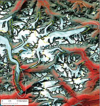
Fig. 2. Raw classification result from the algorithm (black) and manually corrected outlines (yellow) for a small region in the Chugach Mountains (scene A). Circles denote examples of misclassification of water bodies and non-classification of the debris-covered glaciers. A false-color composite (bands 432 as RGB) of the respective Landsat scene is displayed in the background.
In the case of the eastern part of the Chugach Mountains, we first processed the Landsat ETM+ scene from 2002, but later two scenes from 2009 with much better snow conditions became available. As a simple update of the previously mapped extent by digital combination of the 2002 and 2009 outlines was not practical, we completely reprocessed the outlines for this region with the latest imagery.
3.2. Drainage divides
One of the main outcomes of a glacier inventory is a comprehensive set of topographic parameters for each glacier entity (Reference Paul, Kääb, Rott, Shepherd, Strozzi and VoldenPaul and others, 2009). A DEM allows us to create the drainage divides required to clip the contiguous ice masses into individual glaciers (e.g. Reference Manley, Williams and FerrignoManley, 2008; Reference Schiefer, Menounos and WheateSchiefer and others, 2008; Reference Bolch, Menounos and WheateBolch and others, 2010b).
To find the most suitable DEM for calculating the divides, we compared the performance of all four DEMs with each other. In all DEMs the sinks were removed and they were smoothed with a 3×3 median filter to minimize the effect of possible outliers. Then we applied the approach of Reference Bolch, Menounos and WheateBolch and others (2010b) to calculate the divides from the DEMs. For this purpose, a 1 km buffer is created around all glaciers to constrain the hydrological calculations to this buffer. As this method can generate many artificial and very small polygons in the ablation area, these were selected with a spatial query tool and removed. The resulting drainage divides are similar in all DEMs for distinct mountain ridges (deviation <100 m), although the coarser resolution of the SRTM-3 DEM is recognizable (Reference ArendtFig. 3). Large shifts of the location (>1000 m) are observed in the flat terrain of the accumulation areas where low contrast in the optical imagery can introduce errors in the DEM (e.g. Reference Svoboda and PaulSvoboda and Paul, 2009; Reference BolchBolch and others, 2010a). Divides derived by SRTM-1 and SRTM-3 DEMs seemed to be most realistic when visually compared with the satellite data. Larger deviations of the basins as calculated from the GDEM could be attributed to unnatural peaks and sinks which commonly occur in the GDEM (Fig. 3) and which can show a deviation of >±25m compared to the SRTM DEMs (Frey and Paul, unpublished information). In most cases, the ice divides varied by <500m in the accumulation regions. We finally selected the NED DEM because it covered the entire study region and performed slightly better than the GDEM.
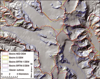
Fig. 3. Comparison of drainage divides derived from the four different DEMs where the background is a shaded relief of the USGS NED.
Visual inspection was used to further improve the resulting divides, especially in the accumulation area where anomalies in the NED DEM also occur. A hillshade raster, a flow direction grid, topographic maps and false-color composites are used additionally for this purpose. After intersection of the drainage divides with the glacier outlines, topographic glacier inventory parameters were calculated for each glacier entity from the NED DEM following Reference Paul, Kääb, Rott, Shepherd, Strozzi and VoldenPaul and others (2009). As mentioned above, minimum elevation was derived from the ASTER GDEM.
3.3. Change assessment
To use the glacier outlines from the DLG for calculation of size changes, we first adjusted the drainage divides created for the glacier inventory to the DLG outlines and then used them to separate the contiguous ice masses. We then manually selected a subset of 347 glaciers in the seven subregions that are suitable to assess area changes. To be suitable, the glaciers in both datasets must be clearly identifiable, which is often not the case (see section 5.2). Because the large glaciers are often calving (in lakes) or are of tidewater type, the resulting selection contains relatively ‘smaller’ glaciers, the largest one being 68 km2. For most of the glaciers, the dates to which the DLG outlines refer were obtained from Reference Berthier, Schiefer, Clarke, Menounos and RémyBerthier and others (2010) or directly from the USGS 1 : 63 000 topographic maps. Because the available DLG outlines have been partly updated, we visually controlled that the selected glaciers were in good agreement with the extents visible on the map (DRG). We are aware that the DLG outlines come with some (maybe systematic) uncertainty, but we think it is worth using them in this study as also recommended by Reference Manley, Williams and FerrignoManley (2008).
4. Results
The glacier inventory of western Alaska includes 8827 glaciers larger than 0.02 km2 and covers a total area of ~16 250km2 (Table 2). The 31 (0.4%) glaciers larger than 100 km2 account for 47% of the total area, while the 7627 glaciers (86%) smaller than 1 km2 account for only 7.5% of the area. These percentages vary with the specific mountain range analyzed, but the general picture is similar in all regions. The strong contrast in the number and size contribution is visualized for the Chugach Mountains in Figure 4. The largest glaciers are also located in this region, but some are also found in the Kenai Peninsula and the Tordrillo Mountains (Table 3). This table also provides selected parameters from the inventory for the ten largest glaciers. Three of these huge glaciers are land-terminating, while seven are calving into lakes or the ocean. In Table 4 the number and area covered for the seven sub-regions is listed along with the mean glacier size in each region. While four regions have an ice cover between 1900 and 2700 km2, that in the Chugach Mountains region is nearly 6500 km2, while in the two smallest regions (Fourpeaked Mountain and Talkeetna Mountains) it is ~340km2. On the other hand, the mean size of the glaciers in each region is similar for five regions (1.1–1.8km2) and only slightly larger for the south Kenai Peninsula and the Chugach Mountains (2.3 and 2.6 km2). This indicates that a region with comparably large glaciers is always accompanied by a proportionally higher number of small glaciers.
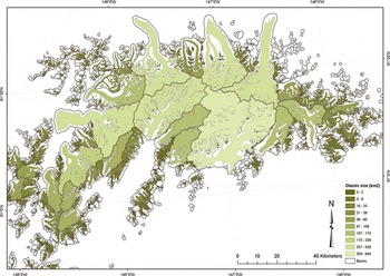
Fig. 4. Color-coded illustration of the glacier size distribution in the Chugach Mountains. Thick lines represent the basins.
Table 2. Summary of glacier count and area value per size class for the entire dataset
Table 3. The ten largest glaciers in the study region (sorted by size) with some topographic parameters
Table 4. Summary of glacier value per sub-region. Region names are from DeLorme (2004)
Figure 5 shows the area–elevation distribution for the seven sub-regions with 100 m binning. While most (84%) of the ice is located between 600 and 2000 ma.s.l., the glaciers in the Chugach Mountains have an elevation range from sea level to almost 4000 m. The much higher mean elevation of the glaciers in the more continental regions, Tordrillo and Talkeetna, is clearly visible. The different curves thus reflect the differences in the topoclimatic conditions.
Fig. 5. Glacier area–elevation distribution (hypsography) for the seven sub-regions (see Fig. 1 for location) with 100m binning.
Mean elevation of a glacier can be seen as a proxy for the equilibrium-line altitude (ELA) that represents balanced-budget conditions (e.g. Reference Braithwaite and RaperBraithwaite and Raper, 2009). It is also a proxy for the climatic conditions in a region, especially precipitation amounts. The spatial analysis of this parameter reveals a strong increase from ~100m at the coast to 3000ma.s.l. in the interior (Fig. 6). To give this visual interpretation more weight, we defined an arbitrary point in the Gulf of Alaska that is located at the end of two sector lines enclosing the region (753200, 655100; World Geodetic System 1984 (WGS84) UTM zone 5N), and calculated the distance from each glacier to this point. A linear regression yields a high correlation (R 2 = 0.91; significance level (p value) 0.003) between this distance (100500 km) and the mean elevation (1000 to nearly 2000 m). This regional trend has of course a high local variability, indicating that changes in temperature and/or precipitation will affect each glacier differently. We have also analyzed the variation of mean elevation with aspect sector for each sub-region (Fig. 7). Apart from the already described increase of mean elevation with distance from the coast, the graph reveals only a small variability with aspect sector (in the mean) in each region, indicating little dependency on this factor. This suggests that the precipitation regime has a much stronger influence on mean elevation in this region than received radiation, at least for the overall trend. On a more regional scale, glacier aspect can also have a more dominant influence on mean elevation (Reference EvansEvans, 2006).
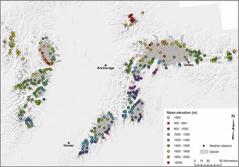
Fig. 6. Spatial variability of mean elevation with size for glaciers larger than 5 km2 over the entire study region. Glaciers are in light grey, and in the background is a shaded relief from the USGS NED. Weather stations are located with black square dots.
Fig. 7. Mean elevation as a function of aspect for each sub-region. (See Table 4 for region.)
In Figure 8 the relative change in glacier area per decade versus glacier size is illustrated for the subsample of 347 selected glaciers. As for several other regions where such analysis has been performed (e.g. for the western Canadian glaciers by Reference Bolch, Menounos and WheateBolch and others, 2010b), a large variability of the changes is found, with an increase in scatter and an increasing relative area loss towards the smallest glaciers. All glaciers in this subsample lost area; the calculated total loss represents ~23% of the initial area (1948–57). (See section 5.2 for discussion of potential uncertainties.) This area loss is in good agreement with the changes found by Reference Barrand and SharpBarrand and Sharp (2010) for Yukon (Canada) glaciers. However, it must be noted that the size-class distribution might be different in our sample, making the two samples less comparable.
Fig. 8. Glacier shrinkage as a function of initial glacier area (1951–57) for a subset of 347 glaciers.
5. Discussion
5.1. Glacier inventory data
Because of the importance of Alaskan glaciers for global sea-level rise (e.g. Reference Kaser, Cogley, Dyurgerov, Meier and OhmuraKaser and others, 2006; Reference Radić and HockRadić and Hock, 2010), most of the recent studies on glacier change in Alaska focus on changes in glacier volume, either for selected glaciers (e.g. Reference ArendtArendt and others, 2006; Reference MuskettMuskett and others, 2009) or entire mountain ranges (e.g. Reference VanLooy, Forster and FordVanLooy and others, 2006; Reference Berthier, Schiefer, Clarke, Menounos and RémyBerthier and others, 2010). Several of these studies could not exclude certain types of glaciers (e.g. calving or surging) from the analysis to better assess the impact of climate change on mass balance, as outlines of individual glaciers in this region have not been available so far. Moreover, Reference Kaser, Cogley, Dyurgerov, Meier and OhmuraKaser and others (2006) highlighted the difficulties of determining the mass balance for an entire mountain range from direct measurements of a few selected and often comparably small glaciers. This is only possible when the representativeness of the measurements for the entire region is clear (e.g. Reference Paul and HaeberliPaul and Haeberli, 2008; Reference Fountain, Hoffman, Granshaw and RiedelFountain and others, 2009). With the outlines now available, we hope that these glacier-specific changes can be calculated.
Though we would have preferred to have all satellite scenes used for the inventory acquired within 1 year (at best) or a few years, we decided to use only the scenes with the best snow conditions (Table 1), in order to minimize the workload and error for manual corrections due to seasonal snow (e.g. Reference Paul and AndreassenPaul and Andreassen, 2009). In the resulting 5 year period, some glaciers (e.g. Columbia Glacier) have shown considerable changes in extent. However, for each glacier outline, the acquisition date is given in the attribute table, so a proper reference for change assessment can be made. This is of particular importance when dates for the comparison dataset also vary strongly (e.g. Reference Andreassen, Paul, Kääb and HausbergAndreassen and others, 2008).
Apart from debris-covered small glaciers or those with an unclear transition to creeping permafrost bodies, the manual correction of the outlines was generally straightforward. This is due to the comparably good contrast of the debris-covered parts with surrounding terrain that results from the low solar elevation at high latitudes. We are aware that the manually corrected outlines of individual (in particular, small) glaciers might have larger errors, but based on previous studies that have determined the accuracy of the outlines (e.g. Reference Paul, Huggel, Kääb, Kellenberger and MaischPaul and others, 2003; Reference Andreassen, Paul, Kääb and HausbergAndreassen and others, 2008) we are confident that for most glaciers the accuracy of the derived area is better than ∓5%. This does not, however, include differences due to a different interpretation of a glacier entity as a whole (e.g. position of drainage divides, tributaries, attached snowfields). For example, in several cases we may have included perennial snowfields in the inventory, as no bare ice was visible on the satellite images. This is a common problem in all inventories (e.g. Reference DeBeer and SharpDeBeer and Sharp, 2009; Reference Paul and AndreassenPaul and Andreassen, 2009), but these elements can be marked in the attribute table (Paul and others, 2009).
Considering the workload involved in editing the automatically derived outlines, we strongly recommend using automated methods for the initial mapping. This also helps to cover the entire sample of glaciers in a region and to create a consistent and reproducible dataset (Reference Svoboda and PaulSvoboda and Paul, 2009). During manual editing, an inconsistent interpretation and certain degree of generalization is applied, i.e. the same spectral properties of a pixel are always interpreted differently. Though this might not have a large influence on the total area of a glacier, overlays of multiple manual digitizations of the same glacier by the same person revealed a considerable variability (∓1 pixel) of the outline position. Comparing outline overlays from several analysts reveals an even higher variability (∓2 pixels or more), i.e. the digitized extent is not reproducible (GlobGlacier, http://www.globglacier.ch/docs/globgl_deliv7.pdf).
The strong dependence of glacier mean elevation on distance from an arbitrarily chosen point in the ocean is very promising for establishing simple parameterization of either ELA or precipitation in high mountain regions. There is virtually no influence of mean glacier aspect sector on mean elevation within a mountain range (Fig. 7), so compared with other regions of the world the influence of reduced global radiation receipts for northerly-exposed glaciers is strongly reduced here (Reference EvansEvans, 2006). We assume that this observation can be explained by the influence of the high annual precipitation amounts on the glacier location as well as by the multi-basin origin of many glaciers which often causes differences in the mean aspect of the entire glacier compared to the ablation region.
5.2. Area change assessment
To calculate area changes, we manually selected a sample of 347 glaciers, as we found several ambiguities between the DLG outlines and our new inventory (Fig. 9). The example in Figure 9 shows that the DLG outlines do not always match the glacier-covered area on the topographic maps, which implies that they must have been updated somehow. Apart from normal retreat with separation of tributaries, we see glaciers that have been mapped in the DLG but not in our inventory (and vice versa in other regions). This could mean that (1) the glacier has disappeared, (2) we failed to map the glacier because of complete debris cover, or (3) in the DLG, seasonal snow was mapped. Hence, despite changes being clearly visible, the outlines of the DLG can rarely be used for automated change assessment. Also for the manual selection performed here, the error bounds are likely large, as cartographers and glaciologists can have different perceptions of what a glacier is, and the ‘truth’ can be a matter of debate, even in the field. For the manual selection used here, these cases can be largely excluded so that our estimate of the relative area loss is probably a lower bound.
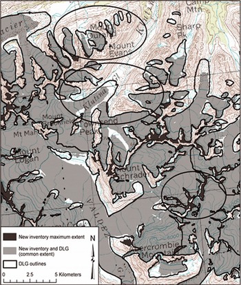
Fig. 9. Illustration of glacier recession in the Valdez district, southern Chugach Mountains. Thick black lines show the DLG glacier outlines, and light grey shading represents the new glacier inventory within the DLG extent, while the dark grey shading depicts the new glacier inventory outside the DLG extent. An example of the DRG (Valdez B-6) is displayed in the background. Black ellipses highlight examples of differences between the two datasets.
Though the link between glacier area change and climate change is less straightforward than for mass-balance or length changes, there are also a number of benefits in assessing the former. Area changes can best be derived from satellite sensors and have thus been determined for many regions of the world. This provides interesting insights into the highly variable behavior of glaciers in different regions (e.g. Reference DeBeer and SharpDeBeer and Sharp, 2009; Reference Paul and AndreassenPaul and Andreassen, 2009). They also provide evidence for changes in surface elevation, for example when area is shrinking along the entire perimeter or new rock outcrops appear (e.g. Reference Paul, Kääb and HaeberliPaul and others, 2007). When this occurs in the accumulation region, the glacier will likely disappear (Reference PeltoPelto, 2010). Area changes of glaciers are thus a valuable proxy for climate-change impact assessment on a global scale.
6. Conclusions
We have presented a new satellite-derived glacier inventory of western Alaska based on nine scenes from Landsat TM acquired between 2005 and 2009. This 5 year period is required because of frequent clouds and seasonal snow on most scenes in the USGS archive. The mapped 8827 glaciers larger than 0.02 km2 cover an area of 16 250 km2, a few of them (31) being >100km2 and most (86% by number) being <1 km2. We found a strong relationship between glacier mean elevation and the distance from the ocean, which is related to the decreasing amount of precipitation inland.
We used the band ratio method (TM3/TM5) with a threshold to automatically map all glaciers in the region. Misclassified lakes or water bodies and the omitted debris-covered parts of glaciers were manually corrected. Drainage divides derived from the NED DEM allowed us to derive watersheds and obtain individual glacier entities and topographic inventory parameters. Because of large changes in the ablation zones, the parameter minimum elevation was calculated from the more recent ASTER GDEM. For a selection of 347 glaciers we found an overall recession of ~23% (by area) between the 1948–57 (DLG) and 2005–09 (Landsat) epochs. Due to several omission and commission errors between the two datasets, a more detailed analysis of the DLG is required before it can be used for further change analyses. In forthcoming studies, we will use the glacier inventory dataset derived here to assess glacier-specific changes. All inventory data are made available in the GLIMS glacier database to enable their use in the required additional studies and assessments.
Acknowledgements
This study was funded by the ESA GlobGlacier project (21088/07/I-EC). Landsat scenes, DLG outlines, DRG maps and the DEM NED were obtained from the USGS (http://glovis.usgs.gov and http://seamless.usgs.gov. The ASTER GDEM is a product of Japan’s Ministry of Economy, Trade and Industry (METI) and NASA and was downloaded from http://www.gdem.aster.ersdac.or.jp and the also used seamless SRTM DEM was downloaded from http://srtm.csi.cgiar.org. We thank E. Berthier for providing data and useful comments on the paper. The comments of the editor, B. Raup, and an anonymous reviewer helped to improve the clarity of the paper.


