Motivation

In the context of glaciological work, radar studies are highly valuable in several respects. Mass-balance parameters such as ice thickness and subglacial topography can be surveyed over wide areas (Reference DrewryDrewry, 1983; Reference Hodge, Wright, Bradley, Jacobel, Skou and VaughnHodge and others, 1990). These parameters are input to numerical models of ice-flow dynamics to derive responses of the polar ice caps to global changes (Reference Huybrechts and OerlemansHuybrechts and Oerlemans, 1990; Reference HuybrechtsHuybrechts, 1994). Moreover, the extent of ice streams, which play an important role in the understanding of the stability of ice sheets (Reference BentleyBentley 1998), can be determined (Reference BellBell and others, 1998). The mapping of internal radio-echo sounding (RES) horizons enables glaciologists to identify optimal sites for deep ice-core drilling (Reference Dahl-JensenDahl-Jensen and others, 1997). With radar systems, the information deduced from ice-core studies (GRIP Project Members, 1993; Reference Grootes, Stuiver, White, Johnsen and JouzelGrootes and others, 1993) can be extrapolated from the drill sites to the whole area covered by radar profiles (Reference Hempel and ThyssenHempel and Thyssen, 1993). For these reasons, the Alfred Wegener Institute (AWI) has operated an airborne RES system for glaciological studies since 1994 in Greenland and Antarctica.

System Design

Radar systems have been used since the 1950s in remote-sensing operations in Greenland and Antarctica (Reference WaiteWaite, 1959). The first measurement of ice thickness with a standard US Air Force radio altimeter SGR-718 is described by Reference Waite and SchmidtWaite and Schmidt (1962). A historical review of radar systems in glaciology is given by Reference Gogineni, Chuah, Allen, Jezek and MooreGoginem and others (1998). An overview of the technical details of different frequently used airborne RES systems can be found in Reference Bogorodsky, Bentley and GudmandsenBogorodsky and others (1985).

Technical Data: High-Frequency Components

AWI operates two Dormer Do 228-100 aircraft that can be equipped with different scientific instruments depending on the various scientific programmes. The system presented here was built by AWI in cooperation with Aerodata FlugmeBtechnik GmbH, Technische Universität (TU) Hamburg-Harburg and the Deutsches Zentrum fur Luft- und Raumfahrt e.V. (DLR). Figure 1 shows the different components of the system, from the signal generator to the data recording and analysis.

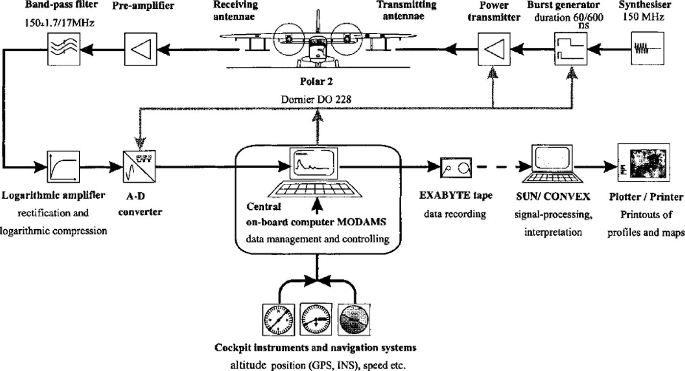
Fig. 1.

Sketch of the AWIRES system.

The transmitted high-frequency (HF) signal is produced by a synthesizer, and the output frequency fo can be chosen in 1 MHz steps between 100 and 200 MHz. In normal operation it is set to 150 MHz with an output power setting of P_synth - 10 dBm. The output frequency fo can also be easily changed during the flight. The limiting factor is the bandwidth of the antennae which is about 20 MHz around the centre frequency of 150 MHz and is far smaller than the bandwidth of the HF components. A timing board based on an oscillator with a reference frequency of 10 MHz controls the signal generation, with pulse lengths τ_p of 60 ns or 600 ns (burst) and a pulse repetition frequency f_p of 20 kHz. In "toggle mode" the pulse length of consecutive traces is switched between 60 and 600 ns. Thus used, the system allows both high resolution and maximum depth-sounding during each flight. The signal is split and fed to four transmitter amplifiers that are mounted in the left wing of the airplane (Fig. 1) and connected to a transmitting dipole for each amplifier. The output power P_A for each amplifier is 56dBm (398W), and the resulting peak power is 62 dBm (1.6 kW). The burst can be damped in 5 dB steps up to a damping of 70 dB. To inspect the operational status of the HF transmission, the power consumption of the transmit amplifiers is monitored on a digital display on the operator console.

Two receiving dipoles and a receiver are mounted on the right wing of the aeroplane. In the receiver, the signals of the two antennae are added. The dynamic range of the received signals is of the order of 120 dB. This can be handled by splitting the received signals into several analogue channels with different pre-amplifications for each channel. The pre-amplifiers are specified as solid-state low-noise components. Each channel is connected to a logarithmic amplifier with a typical gain of 21 mV dB⁻¹, a dynamic range of 75 dB and a corresponding maximum output voltage of 2000 mV. Thus the overall dynamical range is split into different channels. The initial design of the system comprised two analogue channels. In 1997 that was increased to three channels, yielding better resolution especially for low signal strengths. The following technical details refer to the present version; details of the older versions are noted in parentheses.

Both transmitter and receiver antennae are short backfire antennae (Reference RothammelRothammel, 1991) that were adopted for use under the wings of Polar! They consist of a big reflector (the wing itself) and a small reflector with a dipole in between. The small reflectors are held in position by pylons that also carry the folded dipoles. Such an antenna has a high gain (G=14dB_d) but small dimensions.

Data Recording and Visualisation

Each logarithmic amplifier passes the signal to a 12-bit (8-bit) analogue-to-digital (A-D) conversion cascade. For each data sample in the resulting trace a decision is made as to which channel’s data are recorded. The decision is based on the signal strength of the data sample. According to the segmentation of the dynamic range into three channels, there is only one valid channel for each signal strength. The time required for the A-D conversion and the sampling rate of 20 Hz permit 200 averages for each trace. The sampling interval is 13.33 ns and the trace length is 50 Ms. The digitised data are linearised in the central on-board computer, using an anti-logarithm table to minimise the influence of the logarithmic detectors, and then recorded in a Modular Data Acquisition and Monitoring System (MODAMS) format in 24-bit (20-bit) representation on an 8 mm EXABYTE tape. The data rate is about 1.0 OBIT¹. The data are recorded digitally so that enhanced seismic-processing tools can be applied after the flight (Fig. 1). In order to have direct control of the data quality, the user has several options beyond the features depicted in Figure 1. It is possible to display single traces in A-scope format, or to display many consecutive traces in Z-scope format, on an online monitor of the central computer where both the horizontal and vertical axes can be set by the operator. Moreover, a coloured hard copy in Z-scope format is produced every 2 or 4 minutes of flight time (user-selectable). The data are thus preprocessed, resulting in online analogue plots of very high quality. This enables the early identification of areas of special glaciological interest in the field, so that the experiment can be adapted if necessary.

Navigation and Resolution

Included in the MODAMS format are data blocks with additional information such as navigation data. The aircraft positioning is accomplished using an inertial navigation system (INS), barometric altimetry, global positioning system (GPS) and, since 1997, laser altimetry and post-processing differential GPS. The position errors after processing vary between ±100 and ±5 m in horizontal directions and ±50 and ± 5m in elevation, depending on the instruments and methods used. During the surveys the aircraft ground speed is 65 ms"¹ (130knots). Combined with the sample frequency of 20 Hz, a horizontal spacing of the traces of 3.25 m results. In the "toggle mode" the spacing for the traces with the same pulse length is 6.5 m. The theoretical vertical resolution is 5 m for the 60 ns bursts and 50 m for the 600 ns burst.

System Evaluation

The system was developed to penetrate the ice caps both in Antarctica and in Greenland. That means the system must be able to detect bedrock reflections from 4000 m depth. Moreover, the system dynamics should allow for the high-resolution monitoring of internal reflections using the short (60 ns) pulse.

For a homogeneous flat ice sheet of infinite extent resting on a horizontal ground the received power P_r, neglecting the losses due to polarisation and dispersion, can be calculated (Reference Bogorodsky, Bentley and GudmandsenBogorodsky and others, 1985) by

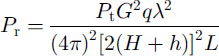
from transmitted power P _t, antenna gain G ² = G _r G _t (where subscripts "r"and " t are receiver and transmitter, respectively), refraction gain q, wavelength A, height of the antenna above the ice surface H, ice thickness h, and the losses involved L. The losses to be taken account of are

where L _A is dielectric loss by two-way propagation through ice, L′_T is transmission loss through the surface, L″_R is reflection loss at the base of the ice sheet and L _K is cable loss. In a pulsed system the relation τ _t = 1/B between receiver bandwidth B and pulse length τ _t holds. The receiver noise N can be calculated as

with noise temperature T = FT ₀, Boltzmann constant k = 1.38 × 10⁻²³ J K⁻¹, amplification noise factor F = 1.38 and absolute ambient temperature standard T ₀ = 290 K (American National Standards Institute/Institute of Electrical and Electronics Engineers Std 161-1971). Following the concept of Reference Bogorodsky, Bentley and GudmandsenBogorodsky and others (1985, p. 51), the thermal noise, picked up by the antenna main beam, and side and back lobes, must be taken into account.

At the receiver output the signal-to-noise ratio due to Equations (1) and (3) is then (P _r = S)

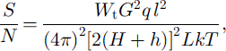
with energy of the transmitter W _t = P _t τ _t.

In the process of the A-D conversion the signals are averaged (stacked). Assuming the stacked data are coherent, the possible maximum gain g _st from this stack is an additional factor on the right side of Equation (4). It can be calculated from the sample interval t and the pulse repetition frequency f _pr as g _st = t f _pr (Reference Ulaby, Moore and FungUlaby and others, 1982). The theoretically possible gain would be g _st = t f _pr = 1000, with t = 0.05 s and f _pr = 20 kHz. The actual gain g _st is 200, due to the time interval needed for A-D conversion.

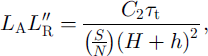
There are two loss parameters (Equation (2)) that are known in general, L _k and L′_T, but the losses are dominated by the product of the unknown losses, the dielectric absorption in ice L _A and the reflection loss L″_R. As L _A increases with increasing ice thickness h, the product L _A L′′_R describes the possibility that the system will detect a reflector with a reflection loss L″_R at depth h. Rearranging Equation (4) and considering the gain g _st due to stacking results in

with

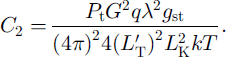
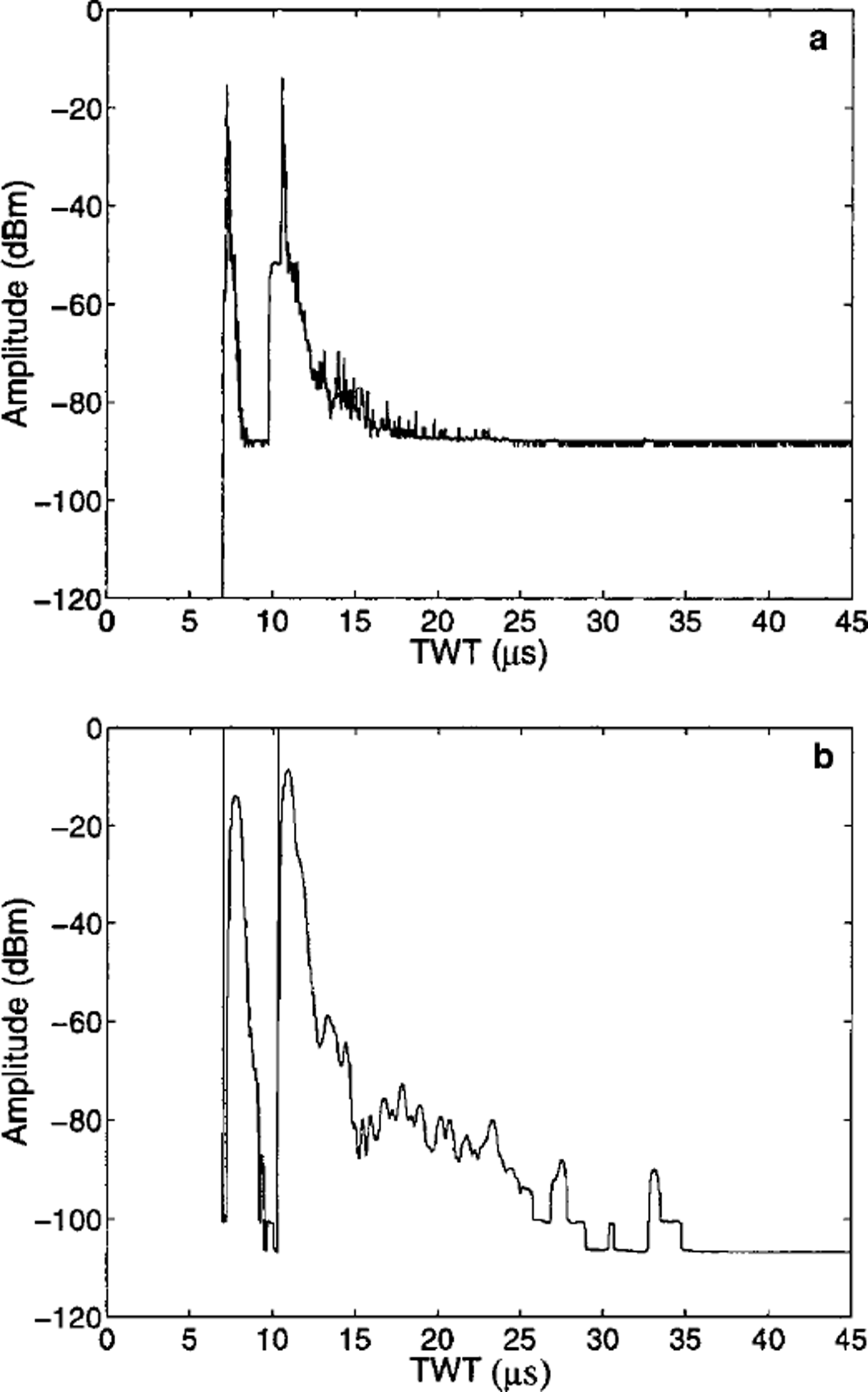
The term C ₂ encapsulates all the constants for a particular system and situation. The actual values of the parameters are P _t = 1585 × 10³ mW, G = 26.3 (= 14.2 dB), q = 2.51 (= 4 dB), λ = 2 m, g _st = 200, L′_T = 1.1 (= 0.4 dB), L _K = 1.99 (= 3 dB), T = 581 K, H = constant = 500 m and S/N = 1.05 This signal-to-noise ratio refers to a clearly detectable reflector marked by an arrow in Figure 5a; the values of the amplitudes can be seen in Figure 6a (signal around 32.5 μs, noise level 35-45 μs). For the present radar the results of Equation (5) are shown in Figure 2. In order to detect a reflector with a reflection loss of 70 dB at, for example, 4000 m, the two-way damping loss must be not more than 74 dB for the 60 ns pulse and not more than 84 dB for the 600 ns pulse.

It is also possible to estimate the dielectric absorption in ice L _A at depth h for a given centre frequency f ₀ and the physical properties of ice (Reference Bogorodsky, Bentley and GudmandsenBogorodsky and others, 1985, p. 12). Defining N _A = 10 log L _A and estimating N _A = 1.65 ×10⁻² h (dBm⁻¹) for an ice temperature T _ice = −15°C, we consider this absorption in Equation (5) dividing by L _A. The result is shown in Figure 3, with the reflection coefficient r defined as

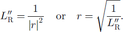
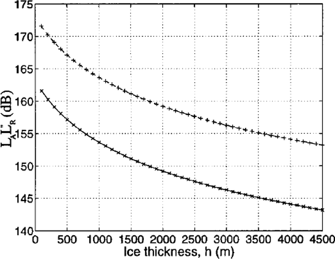
Fig. 2.

Product of the losses L_AL″_R (dB) vs ice thickness h (Δh = 100 m; 100m < h < 4500 m) for the 60 ns burst (×) and the 600 ns burst (+).

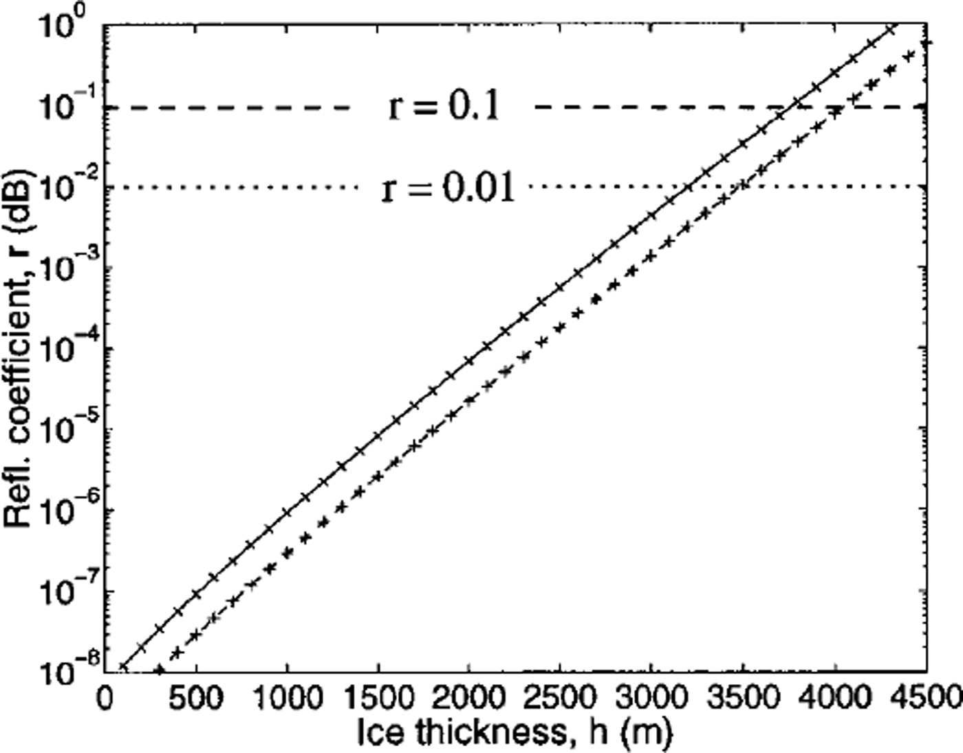
Fig. 3.

Reflection coefficient r vs ice thickness h (Δh = 100 m; 100m < h < 4500 m) for the 60 ns burst (×) and the 600 ns burst (+).

The crosses mark the minimum values for a reflection coefficient r of a given reflector to be detected in the corresponding depth by our system. A reflector with a reflection coefficient r = 0.01 can be detected down to 3200 m depth applying the short (60 ns) pulse, and to 3500 m depth applying the long (600 ns) pulse. The reflection coefficients for the ice-rock transition range from r = 0.05 to r = 0.1 (Reference BlindowBlindow, 1986). An ice-rock interface with a reflection coefficient of r = 0.1 can be detected at little more than 4000 m depth by the long (600 ns) pulse, and at about 3700 m depth by the short (60 ns) pulse. This is only a rough estimation of the system capabilities for a given ice temperature of-15°C and ideal geometry, and neglecting losses due to polarisation and dispersion. The actual capabilities may even be better, because the dielectric absorption in ice decreases with decreasing temperature (Reference Bogorodsky, Bentley and GudmandsenBogorodsky and others, 1985). The mean ice temperature in the central parts of Antarctica and Greenland, where ice thicknesses of > 3000 m are observed, is less than −15°C. The system sensitivity, P _t/(P _r)_min (Reference Bogorodsky, Bentley and GudmandsenBogorodsky and others, 1985), is 190 dB, with a minimum detectable signal strength N _A(P _r)_min of-105 dBm, peak power of 62 dBm and a system-inherent gain of g _st = 200. Stacking in the post-processing phase can enhance the gain even further.

Results

The presented system has been operated successfully in Antarctica and Greenland since 1994, with a total of about 10₅ km of profiles flown. Figure 4 shows a map of the profiles flown in Antarctica that have been processed so far.

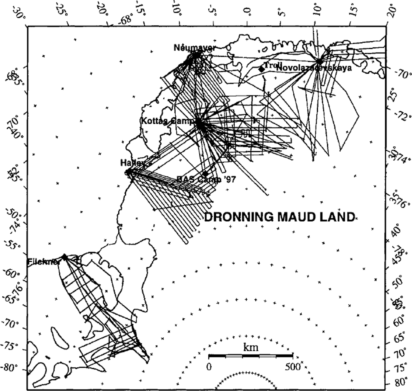
Fig. 4.

Map of RES flight tracks in Antarctica.

In its first Antarctic season the system was operated on the Ronne Ice Shelf (RIS). In the central part of the RIS, data have been collected that can be compared with those from a radar operated by the University of Münster (Reference Hoppe and ThyssenHoppe and Thyssen, 1988; Reference ThyssenThyssen, 1988). This comparison was carried out in the first phase of the Antarctic Bedrock Mapping Project (BEDMAP), sponsored by the Scientific Committee of Antarctic Research (SCAR). The ice thicknesses deduced from both systems agreed generally within several metres. Differences of > 50 m have been observed only at a few locations where the bed topography was steep and the difference in ice thicknesses reflects mainly the errors in the determination of the flight positions. In the second part of that season the system mapped ice thicknesses on the southern boundary of the RIS for a mass-balance study (Reference Lambrecht, Mayer, Oerter and NixdorfLambrecht and others, 1999). In accordance with Reference BellBell and others’ (1998) result, we found that the internal reflectors in the area of an ice stream are disturbed and that it can be difficult to determine the position of the grounding line with RES data only (Reference LambrechtLambrecht, 1998). Yet from the airborne measurements of both ice thickness and surface elevation the position of the grounding line of the Foundation Ice Stream was deduced. It was found that this position is some 40 km further south than formerly supposed, so the area of the RIS is about 1700 km² larger than previously thought (Reference Lambrecht, Mayer, Hempel, Nixdorf and OerterLambrecht and others, 1997). Finally, new mass-flux calculations that resulted in ice-stream transport from the inland ice into the eastern ice shelf of 51 km³ a⁻¹ are partly based on the airborne RES data (Reference Lambrecht, Mayer, Oerter and NixdorfLambrecht and others, 1999). Given that this area is heavily crevassed, and thus inaccessible in parts, the RES data are of great value.

The system has since been used to determine ice thicknesses and internal ice layers in Dronning Maud Land (DML), Antarctica (Reference Steinhage, Nixdorf, Meyer and MillerSteinhage and others, 1999). This work was carried out in the frame of the European Project for Ice Goring in Antarctica (EPICA) pre-site survey (Reference Oerter, Graf, Wilhelms, Minikin and MillerOerter and others, 1999) in order to identify an optimal site for deep ice-core drilling. Data examples from the DML surveys of different years collected on a test profile flown with the 600 ns pulse applied are shown in Figure 5a and b. For details of the data processing and visualisation see Reference Steinhage, Nixdorf, Meyer and MillerSteinhage and others (1999). Data gathered with the earlier system with a 17 MHz analogue filter applied during data collection are shown in Figure 5a. Data collected with the present system with a 1.7 MHz analogue filter applied during data collection are shown in Figure 5b. The horizontal axis shows along-track distance referenced to an arbitrary starting-point. The vertical axis refers to the two-way travel time (TWT) of the radar signals in μs. The ice surface can be detected at about 10 Ms TWT, and the reflections from the bed can be seen at 28–38 μs, indicating that the subglacial bed has a very pronounced topography. In Figure 5a, horizontal lines are observed at 30–50 μs, especially near 35 μs; these lines are due to system-noise sources. These sources have been eliminated in the new design as shown in Figure 5b, where the horizontal lines are absent in that time range. The reduction of internal and external noise, as well as the enhanced resolution, lead to a much lower detection level, resulting in a continuous reflection from the subglacial bed in Figure 5b compared to the reflection gaps in Figure 5a.

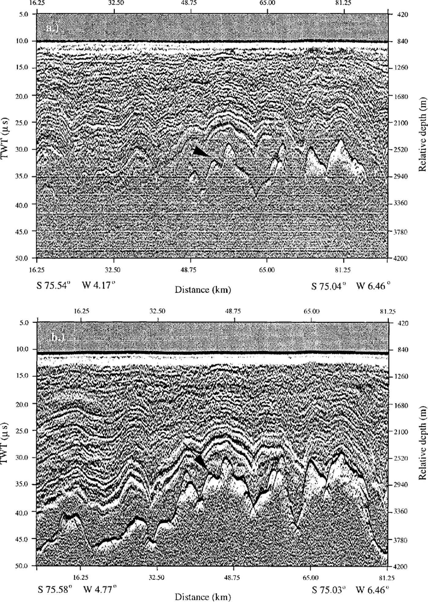
Fig. 5.

(a) Test profile section of 1997. The position of the extracted trace in Figure 6a is indicated by the arrow at 53.55 km. The origin of the x axis is arbitrarily chosen, and the coordinates of the start and end points of the profile are noted at the bottom. A static correction has been applied, so the surface, indicated by the first reflection, is located at slightly less than 10 μs TWT (at a relative depth of 840 m). Bed reflection can be observed at 35 μs TWTstarting at a distance of 48 km and continuing along the profile. The depth conversion of the TWT was calculated using a velocity of 168 m⁻¹, neglecting any firn correction. The thin horizontal parallel lines with a separation of approximately 4 μs are due to system noise, (b) Test profile section of 1998, flown in the same direction but at a slightly higher flight level than the section presented in (a). The coordinates of the start and end points of the profile are noted at the bottom. For details of x axis, static correction and depth conversion see (a). In this section the bed reflections can be observed along the whole profile, revealing a mountain range with differences in height of >1200 m within <20 km. The location of the extracted trace of Figure 6b is indicated by the arrow. Due to the system improvements there is no obvious system noise.

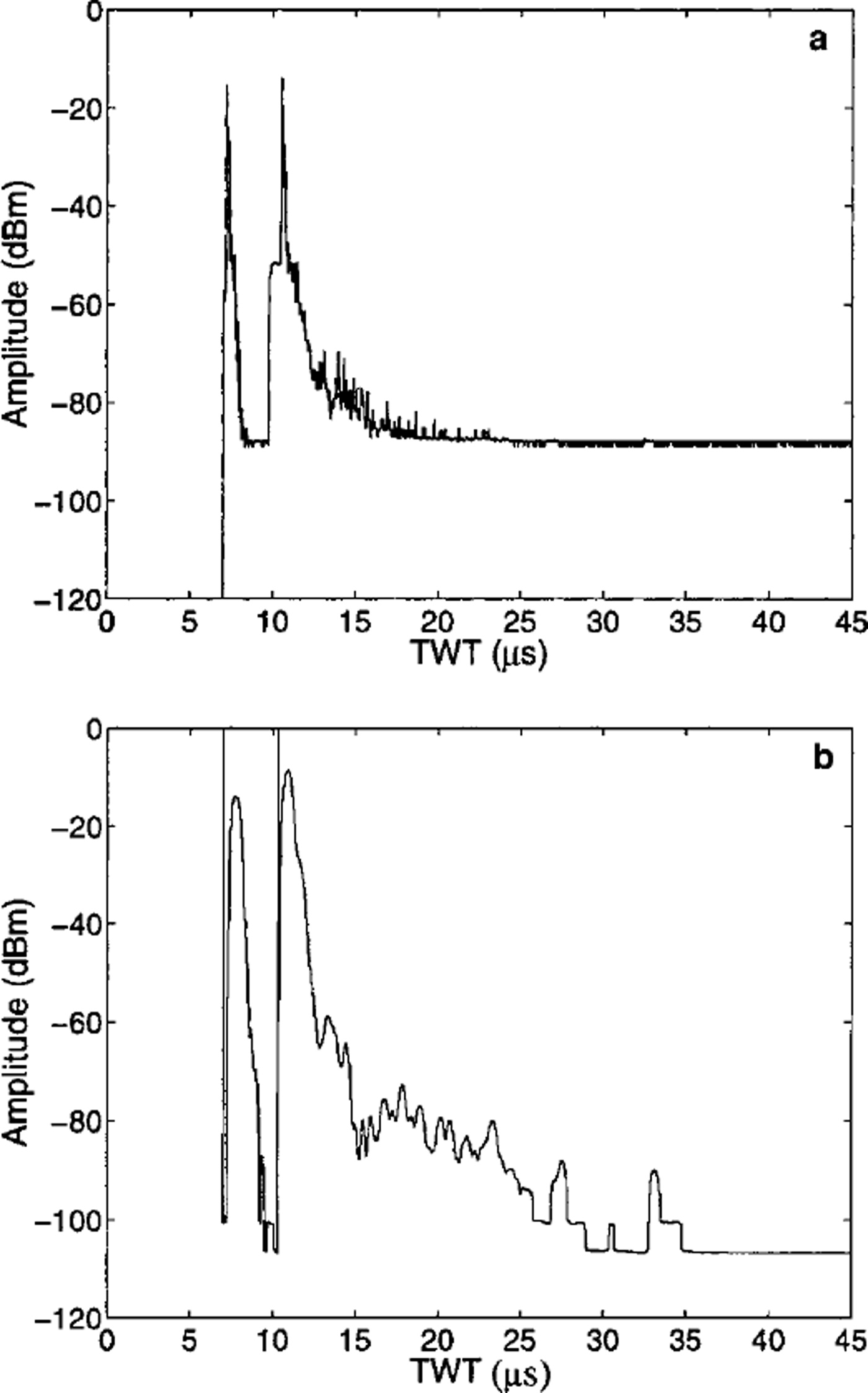
The system detection level can be quantified by calculating signal strengths. The amplitudes of single traces showing a reflection from the top of a small hill (Fig. 5; marked there with an arrow) are shown in Figure 6. Figure 6a shows the trace from Figure 5a. Figure 6b shows the trace from Figure 5b. The vertical axis in Figure 6 refers to the signal strength at the output of the receiving antennae, and the horizontal axis shows the TWT. The reflection from the ice surface can be seen shortly after 10 μs TWT, and the reflection from the hill can be seen at 32 μs TWT. In the earlier radar (Fig.6a) the signal barely exceeds the noise level of about −89 dBm, whereas in the present version the reflection from the hill is almost 20 dB above the noise level of −106 dBm.

Fig. 6.

(a) Single trace of profile shown in Figure 5a. For location see the arrow in Figure 5a. (b) Single trace of profile shown in Figure 5b. For location see the arrow in Figure 5b.

This area was chosen as a test region because of the poor reflection quality of the bed. Comparing Figures 2 and 3 with Figures 5 and 6, it can be seen that the predicted system performance and the actual detection capabilities are in general agreement. The maximum ice thickness detected in Greenland is about 3400 m (Reference Hempel and ThyssenHempel and Thyssen, 1993). In 1994, in the first season of the RES system, the reflection from the bed could be detected with the 600 ns pulse without further data processing and could be seen on almost every profile on the online plot during the flight. The reflections there could be detected with the 60 ns pulse after tenfold stacking at an ice thickness around 3000 m. Up to now the deepest reflector resolved by the RES was the subglacial bed on profiles south ofjutulstraumen, with a maximum ice thickness of > 3600 m (Reference Steinhage, Nixdorf, Meyer and MillerSteinhage and others, 1999). Since 1994 the system has been improved, and it was successfully used in the frame of the EPICA pre-site survey. As a result, new maps of ice thickness and subglacial topography in DML were created, details of which are discussed in Reference Steinhage, Nixdorf, Meyer and MillerSteinhage and others (1999). The survey covered an area of 9.48 × 10⁵ km². Compared to the ice-thickness maps published before (Reference DrewryDrewry, 1983), it is clear that the ice is much thicker, maybe 100-150 m on average, in western and central DML (Reference Steinhage, Nixdorf, Meyer and MillerSteinhage and others, 1999). In addition, there is no smooth distribution as mapped before.

An example of the capabilities of the system to map internal structures in DML with the short (60 ns) pulse is given in Figure 7. Internal layers can be tracked continuously for several tens of km. Single layers can be recognised 200-1800 m below the ice surface. At the end of the profile, seven layers can be seen in the range 2100-2520 m of relative depth. This means that the distance between distinct layers is about 60 m. The vertical resolution can be raised by plotting the profiles with higher vertical exaggeration. Internal reflectors in the ice are related to changes of the complex permittivity. Reference Bogorodsky, Bentley and GudmandsenBogorodsky and others (1985) review the variety of mechanisms discussed by many authors. Changes in density or acidity of the ice resulting from surface processes are most likely, so that internal layers can be seen as isochrones. These isochrones, which tend to follow the bed topography especially in deeper layers (Fig. 7), can reveal some historical aspects of the ice, such as basal melting (Reference Dahl-JensenDahl-Jensen and others, 1997) or the accumulation history (Reference Nereson, Waddington, Raymond and JacobsonNereson and others, 1996).

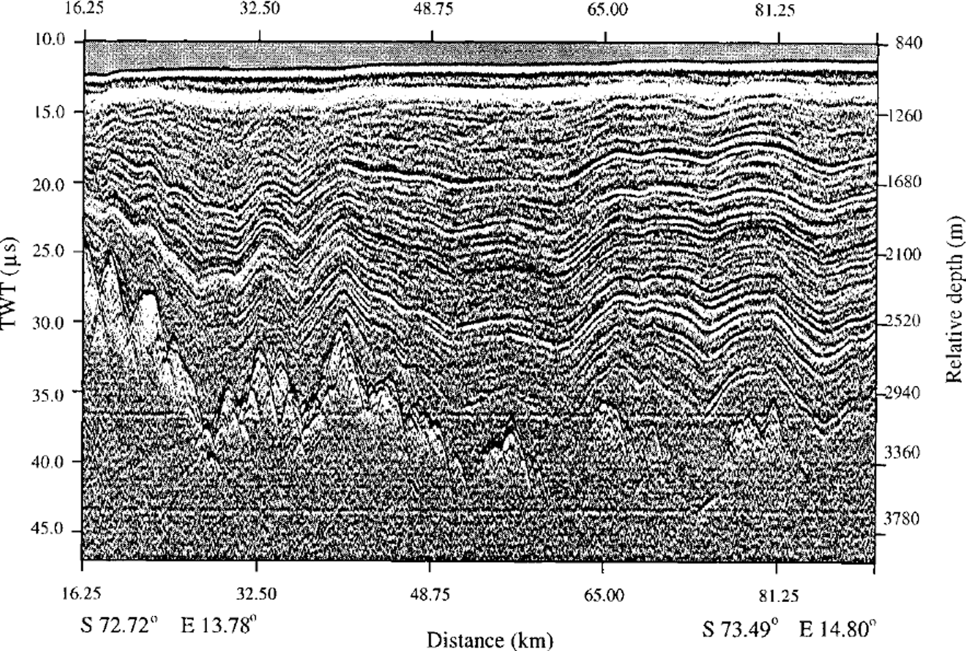
Fig. 7.

Section with enhanced fine structure of internal reflections. Until 40 km just a few bed reflections can be observed. With increasing profile length the rising bed can be seen. The internal reflections show the strongly smoothed height variations of the bed. A static correction has been used to show the bed in its natural position.

Only with an airborne system was it possible with reasonable logistical effort to determine ice thickness and internal ice layers in those large and remote areas where little knowledge existed before (Reference DrewryDrewry, 1983). With the new DML dataset (Reference Steinhage, Nixdorf, Meyer and MillerSteinhage and others, 1999) and the detection capabilities demonstrated in Figure 7, it will be possible to search for and perhaps identify areas with sufficiently thick ice and undisturbed layering in the vicinity of an ice divide. This will be of great value in the EPICA pre-site survey. Moreover, with the data recorded with this system it will be possible to compile three-dimensional surveys of internal layers in DML. A comparison between internal horizons and deep ice-core data will have the perspective to explain past and present changes of, for example, accumulation histories (Reference Nereson, Waddington, Raymond and JacobsonNereson and others, 1996).

Conclusions

AWI has developed a new airborne RES system with a centre frequency of 150 MHz and a peak power of 1.6 kW. Short backfire antennae were designed especially for use under the wings of Polar2. Such an antenna has a high gain but small dimensions. To handle the dynamic range, the received signals are separated into three (two) analogue channels. Each channel’s data are passed to a logarithmic amplifier and to a 12-bit (8-bit) A-D cascade, so that the data are recorded digitally The time required for the A-D conversion and the sampling rate of 20 Hz permit 200 averages for each trace. With the system’s parameters the predicted performance of the radar shows that it should be able to penetrate ice thicknesses of up to 4 km. The system evaluation and the actual system capabilities are in general agreement: a maximum ice thickness of > 3600 m was detected (Reference Steinhage, Nixdorf, Meyer and MillerSteinhage and others, 1999). In a new "toggle mode" the burst duration can be switched between 60 ns and 600 ns for consecutive pulses. Thus used, the system allows both high resolution and maximum depth-sounding during each flight. An on-board pre-processing yields online analogue plots of very high quality. Thus it is possible not only to check the data quality but also to identify areas of special glaciological interest in the field. The system worked reliably on more than 420 flight hours. It was used in a mass-balance study (Reference Lambrecht, Mayer, Oerter and NixdorfLambrecht and others, 1999) to locate the position of the Foundation Ice Stream and to map ice-thickness variations along that ice stream (Reference Lambrecht, Mayer, Hempel, Nixdorf and OerterLambrecht and others, 1997). In the frame of the EPIGA pre-site survey the system was used to find optimal sites for deep ice-core drilling. As a result of that survey, new maps of ice thickness and subglacial topography in DML have been produced (Reference Steinhage, Nixdorf, Meyer and MillerSteinhage and others, 1999). Thus the system has proved to be a valuable tool in a pre-site survey and in mass-balance studies. A comparison between internal horizons, already recorded with this system, and deep ice-core data will provide the perspective to understand past and present changes, such as those of accumulation histories.