


INTRODUCTION
The Antarctic fast ice forms around the coast typically within 150 km from the shoreline or ice-shelf edge (Giles and others, Reference Giles, Laxon and Ridout2008). In winter the fast ice comprises 5% and in summer 35% of the overall Antarctic sea-ice area (Fraser and others, Reference Fraser, Massom, Michael, Galton-Fenzi and Lieser2012). As an annual mean, fast ice accounts for a large fraction of the total sea-ice volume off East Antarctica (Giles and others, Reference Giles, Laxon and Ridout2008). Fast ice is an important component of the Antarctic climate system, in particular by preventing or strongly reducing the exchange of momentum and energy between the ocean and atmosphere (Heil and others, Reference Heil, Allison and Lytle1996).
As fast ice is immobile, either attached to the coast line/shelf edge or grounded to the shallow sea floor, thermodynamic processes dominate fast ice evolution until its breakup, which is typically due to by waves, tides, winds, or strong ocean currents. Until the breakup, the major driving forces for the heat and mass budgets of fast ice and its snow pack are the mass flux by precipitation, shortwave and longwave radiative fluxes, turbulent air-ice fluxes of sensible and latent heat, conductive heat flux through ice and snow, as well as oceanic heat flux (Heil and others, Reference Heil, Allison and Lytle1996; Heil, Reference Heil2006; Lei and others, Reference Lei, Li, Cheng, Zhang and Heil2010; Yang and others, Reference Yang2015). Long-term observations have indicated that the seasonal mean winter air temperature and wind speed have a significant negative correlation with the annual maximum fast ice thickness (Heil, Reference Heil2006). In the Antarctic, accumulated precipitation often results in a snow pack thick enough to generate snow-ice formation due to flooding of ocean water on top of ice. In addition, refreezing of melted snow often results in superimposed ice formation (Kawamura and others, Reference Kawamura, Oshima, Takizawa and Ushio1997). Due to drifting and blowing snow, the snow pack on the fast ice often varies a lot over small spatial scales (Lei and others, Reference Lei, Li, Cheng, Zhang and Heil2010). The oceanic heat flux has a strong seasonal variation in the coastal zone (Heil and others, Reference Heil, Allison and Lytle1996), which strongly affects fast ice mass balance. It is one of the major thermodynamic factors to determine whether a fast ice floe will be transformed from first-year ice (FYI) to second-year ice (SYI) (Yang and others, Reference Yang2015). Thermodynamic studies on Antarctic fast ice have addressed, among others, thermal properties of ice (Pringle and others, Reference Pringle, Trodahl and Haskell2006) and platelet ice formation (Hoppmann and Nicolaus, Reference Hoppmann and Nicolaus2012). In order to better understand the role of sea-ice component in the global climate system, the Antarctic Fast-Ice Network (AFIN) has been initiated a few years ago and various observation sites have been added to the AFIN around the Antarctic continent (Heil and others, Reference Heil, Gerland and Granskog2011).
In the Prydz Bay, off East Antarctica, frazil ice formation is the starting point of fast ice formation (He and others, Reference He, Sun and Wu1998). The ice column mainly consists of columnar ice, but the fraction of granular ice can be as large as 24% (Tang and others, Reference Tang, Qin, Ren, Kang and Li2007). Usually, fast ice in the Prydz Bay reaches a thickness of ~0.3 m before breakup (Heil and others, Reference Heil2006; Lei and others, Reference Lei, Li, Cheng, Zhang and Heil2010). Via formation of snow ice and superimposed ice, snow contributes to the thickness of the multi-year fast ice (Tang and others, Reference Tang, Qin and Ren2006). The maximum FYI thickness ranges from 1.5 to 1.8 m by the end of October. The multi-year fast ice thickness can even exceed 3 m (filed records in the east part of Nella Fjord). The long-term fast ice observations in the Prydz Bay were initiated in summer 2005/06 (Lei and others, Reference Lei, Li, Cheng, Zhang and Heil2010). Since then, the fast ice measurements have been made on annual basis. In March 2012, for the first time, we observed the growth of FYI floe and simultaneous ablation of SYI floe side-by-side in the Prydz Bay. In this paper, we investigate the heat and mass balance of both FYI and SYI floes applying a 1-D thermodynamic sea-ice model. The objective of this study is to understand quantitatively the physical mechanisms responsible for the opposite evolutions of ice mass balance in the Prydz Bay during the summer/autumn transition.
OBSERVATIONS AND METHODS
Study site
The Chinese Zhongshan station, located at 76°22′W, 69°22′S in the Prydz Bay is manned year-round (Fig. 1). A field campaign was carried out on sea ice during summer 2011/12. An automatic weather station (AWS) was deployed on an ice floe. The surface air pressure (P a), wind speed (V a) and direction (V d), air temperature (T a), and relative humidity (Rh) were measured on an hourly basis. The cloud cover (CN) was observed visually every 6 h. A downward-looking Infrared Radiometer sensor (SI-111, CSI) was installed to measure the ice-surface temperature. The fieldwork was part of the AFIN activities in Zhongshan station.

Fig. 1. (a) The Prydz Bay and Zhongshan Station in East Antarctica; (b) P1 and P2 are observation sites for FYI and SYI, respectively. The white dot marks the location where the photos (Fig. 2) were taken, and the dashed lines show the area covered by photos.
Snow and ice observations
A manually operated Canon 450-D camera facing north-northwestwards at the shore was used to record the Nella Fjord surface. The surface melt was visible in early December (Fig. 2a), and melt ponds were seen in late December (Fig. 2b). The melting was further enhanced in January when many puddles were formed (Fig. 2c). The fjord inlet was partly ice free after a storm event on 23 January (Fig. 2d). The remaining ice floe did not break-up and survived to become SYI. A large part of the fjord inlet remained open for ~20 days before refreezing in early February (Fig. 2e). The entire fjord closed up by the end of February (Fig. 2f). From March onward, the fjord was covered by solid ice. The measurements started from 11 March (Fig. 2g). The ice thickness and snow depth were measured at two sites P1 and P2 110 m apart from 10 March to 22 May and from 27 July to 11 December every 2–3 days. Each time, ice thickness and snow depth were measured from five boreholes along a 10 m transect at each site. The accuracy of the measurements was 0.01 m. Snowfall occurred occasionally, but strong winds blew the accumulated snow away shortly after each snowfall event. From early April onwards ice was in a growth phase at both sites (Fig. 3a). The maximum ice thickness reached 1.60 m and 1.67 m at P1 and P2, respectively, in late October before the melting season started. The observations ended in early December.

Fig. 2. Evolution of fast ice from December to March.

Fig. 3. The observed average ice thickness (a) from March to November and (b) in March at sites P1 (black dots) and P2 (circles). The vertical bars denote the spatial standard deviation.
Interesting phenomena occurred in March (Fig. 3a). The ice thickness increased from 0.22 to 0.38 m at P1, but decreased from 1.16 to 0.57 m at P2 (Fig. 3b). The ice surface was dry and no surface melting was detected. At P1, spatial variability of ice thickness on a horizontal scale of 10 m was small, with a standard deviation (STD) of 0.01 m, indicating a fairly smooth ice bottom. At P2 the time-averaged spatial STD of ice thickness was 0.05 m, and the largest STD was 0.14 m on 23 March. During drilling, we experienced internal gap layers, i.e. a sudden drop of the drill bit occurred at the depth of ~0.6–0.8 m below the surface. Similar drilling experiences have been encountered in other seasons in the same region (Hongwei Han, personal communications). The ice growth rate in March was 8 × 10⁻³ m d−1 at P1 and −27 × 10−3 m d−1 at P2.
Sea-ice model
A high-resolution thermodynamic snow and ice model HIGHTSI was applied to simulate sea-ice mass balance at P1 and P2 sites. HIGHTSI is a vertical 1-D model (Launiainen and Cheng, Reference Launiainen and Cheng1998). To solve the surface heat and mass-balance equation, the downward shortwave and longwave radiative fluxes are parameterized according to Shine (Reference Shine1984) and Prata (Reference Prata1996), respectively, taking into account the solar zenith angle, as well as the observed cloud cover, air temperature and air humidity. The surface albedo is parameterised according to Briegleb and others (Reference Briegleb2004). The penetration of solar radiation within snow and ice was adapted from Grenfell and Maykut (Reference Grenfell and Maykut1977) using a two-layer scheme (Launiainen and Cheng, Reference Launiainen and Cheng1998), which ensures the quantitative calculation of sub-surface snow and ice melting (Cheng and others, Reference Cheng, Vihma and Launiainen2003, Reference Cheng, Vihma, Pirazzini and Granskog2006, Reference Cheng2008). The turbulent surface fluxes of sensible and latent heat are calculated, taking the atmospheric stratification into account (Launiainen, Reference Launiainen1995), on the basis of the observed (AWS) wind speed, air temperature and air humidity as well as the modelled ice surface temperature. A heat conduction equation is applied to calculate the evolution of snow and ice temperature profiles. The freezing and melting at ice bottom are controlled by the balance between the conductive heat flux upwards from the ice bottom and the oceanic heat flux to the ice bottom.
The model experiments covered the period from 10 to 31 March 2012. In March, the monthly mean air temperature was −9.1°C and the average wind speed was 8.5 m s−1 mainly from the east. The sky was mainly overcast but occasionally clear. On 14 March, a snowfall event was caught during measurement. A 2 cm snow was accumulated but blown away within a day. In the rest part of March, there were no major snowfall events. This was confirmed by the monthly average precipitation observed in nearby Russian Progress Station. This short appearance of snow is unlikely to have a major impact on sea-ice thermodynamics. Therefore, snow was not taken into account in the model experiments. Model parameters are summarized in Table 1.
Table 1. The model parameters applied in this study

RESULTS AND DISCUSSION
FYI simulation
In cold conditions, especially when the ice is thin, a linear temperature profile between the near-surface air (T a) and the ice bottom (T b) is adequate as an initial condition. The modelled ice thickness well followed the observed evolution (Fig. 4a). The measurements suggested a 0.16 m ± 0.01 m ice growth in March, while the modelled value was 0.158 m. During early ice growth season, one can assume that the latent heat release due to ice formation equals the conductive heat flux through the ice. This is the basic principle of the classical Stefan's Law, which provides an analytic first-order estimate of ice growth. The analytical model can take into account the effect of oceanic heat flux (Leppäranta, Reference Leppäranta1993; Lei and others, Reference Lei, Li, Cheng, Zhang and Heil2010), but the flux magnitude is often very uncertain. Under an average surface air temperature of −9°C and an oceanic heat flux of 30 W m−2, with sea-ice density of 917 kg m−1, thermal conductivity of 2.2 W m−1 K−1, and latent heat of fusion of 333.4 kJ kg−1, the analytical model (Leppäranta, Reference Leppäranta1993) resulted in 0.17 m ice formation, which is well in line with the observations. A change of ±5 Wm−2 of F w as input for HIGHTSI resulted ~−0.02 to 0.03 m changes of basal freezing. The modelled ice temperature regime (Fig. 4b) suggested an upward heat flux throughout the ice layer during the entire simulation period.

Fig. 4. The observed (dots) and calculated (lines) ice thickness at site P1. (a) Model experiments using F w of 30 W m−2 (solid line), 25 W m−2 (dashed line), and by the analytic model (thin solid line). (b) Temporal evolution of the modelled in-ice temperature profile.
SYI simulation
On 10 March the ice was 1.16 m thick at the SYI site. Assuming a linear initial in-ice temperature profile (Fig. 5) from the ice surface (T a) to ice bottom (T b) and an oceanic heat flux of 30 W m−2, the model experiment indeed produced basal ice melt of 0.13 m (Fig. 6, E1), but this was much less than the observed value. Since surface melting was not observed, there must have been some other mechanisms generating more ice melt.

Fig. 5. The initial in-ice temperature profile for the FYI model experiment (black) and SYI model experiments E1 (red) and E2 (blue). The blue line is based on measured in-ice temperature profile for FYI in March (Lei and others, Reference Lei, Li, Cheng, Zhang and Heil2010). The green line is the modelled in-ice temperature of January from Yang and others (Reference Yang2015).

Fig. 6. The modelled (lines) and observed (dots) ice thickness at P2 site.
A previous study on fast sea ice in the Prydz Bay (Lei and others, Reference Lei, Li, Cheng, Zhang and Heil2010) suggested that an in-ice temperature profile in December is highly nonlinear with a large gradient (warm surface) in the upper ice layer and a rather isothermal profile close to the ice bottom. In March, the temperature decreases upward in the upper parts of the ice column, but the lower part is isothermal close to the melting point. Hence, we configured an initial in-ice temperature profile, corresponding to early March conditions on the basis of previous observation and modelling studies (Lei and others, Reference Lei, Li, Cheng, Zhang and Heil2010; Yang and others, Reference Yang2015). With such an in-ice temperature profile, the modelled total ice melting increased to 0.37 m (Fig. 6, E2). Both bottom and internal melt contributed to the increase.
In E1, the modelled in-ice temperature profiles indicated a downward temperature gradient at a lower part of the ice floe near the ice bottom (Fig. 7a). The upward conductive heat flux was, however, smaller than the upward oceanic heat flux resulting in a basal melt of sea ice. For E2, a thick layer above the ice bottom was isothermal for most of the time in March (Fig. 7b), and the oceanic heat flux was accordingly entirely used for basal melt on the ice, which reached a total of 0.17 m in March. When the ice surface cooled, the temperature gradient between the surface and lower ice layers increased, enhancing the upward heat conduction and slowing down the basal melt.

Fig. 7. The modelled in-ice temperature regimes for experiments E1 (a) and E2 (b). The zero in the vertical coordinate refers to ice surface.
The rest 0.2 m of melt modelled in E2 was due to internal ice melt caused by absorbed solar radiation. Averaged over the modelling period, the parameterized downward shortwave radiative fluxes were 120 W m−2 for clear-sky and 36 W m−2 for partly cloudy or overcast conditions. The solar radiation penetrating down to the lower half of the ice layer reached up to 11 W m−2 (Fig. 8) and generated internal melt. Figure 9 illustrates the depths and the diurnal cycle of active internal ice melt. The layer was 0.6–0.8 m below the ice surface in agreement with the observed occurrence of intermediate soft ice encountered on 12 and 13 March. The internal melt stopped ~22 March because the sky turned to overcast, solar zenith angles increased and, accordingly, less solar radiation was available at the surface. Another factor contributing to the end of internal melt was the gradually enlarged conductive heat flux in ice.

Fig. 8. The average penetrating solar radiation below blue ice surface during the modelling period, calculated applying a two-layer parameterization (Launiainen and Cheng (Reference Launiainen and Cheng1998); Table 1) for SYI site. The depth in x-axis is normalized with respect to the ice thickness.
Fig. 9. The observed (dots) and modelled (black line) ice thickness (E2). The white area above the ice bottom indicates the depths and periods of active internal melt of ice.
The modelled ice thickness of E2 was 39% more than observed by the end of March. The large uncertainty of SYI modelling experiment originates from the in-ice temperature profile assumption, which was made in lieu of observations. Therefore, we carried out a number of model experiments to study the sensitivity of in-ice isothermal depth to the ice mass balance. The assumed initial in-ice temperature profiles are presented in Fig. 10. The model forcing was the same as in E2.

Fig. 10. The in-ice temperature profiles applied as an initial condition for model simulations.
Enlargement of the in-ice isothermal layer generated more ice melt mainly inside the ice (Fig. 11). The basal ice melt was not affected by the thickness of the isothermal layer because the oceanic heat flux remained the same for those model experiments and even a thin isothermal layer prevents heat conduction upwards of the ice bottom.
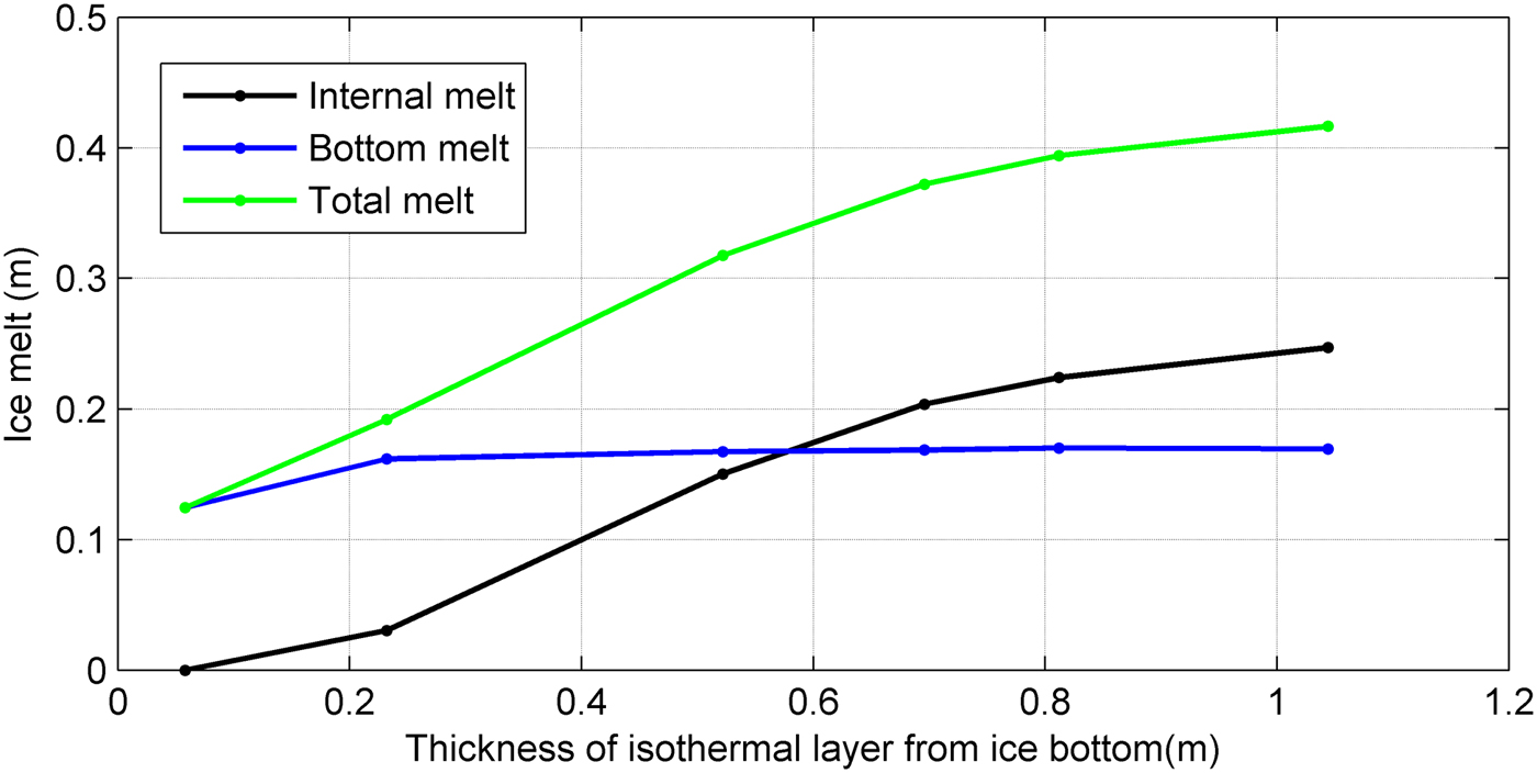
Fig. 11. Modelled ice melt components at SYI site as a function of the thickness of the in-ice isothermal layer upwards from the ice bottom.
Other uncertainty may be associated with the solar radiation available at the surface. For example, a reduction of surface albedo from 0.55 to 0.40 would increase the internal melt from 0.202 to 0.245 m (Fig. 12). The manual CN observations may also generate uncertainty in the modelled internal melt.

Fig. 12. The modelled accumulated internal melt for E2 (black) and for a sensitivity experiment, where the surface albedo was set to 0.40 instead of 0.55 as in E2.
An increase of F w would naturally enhance the basal melt (see the section FYI simulation). The water depths at P1 and P2 were 10 m and 12 m, respectively. The F w should not differ much between them. However, we have no information on the correct value of F w at P2. When P1 was open in January and February, the downward solar radiation directly heated the sea water. In the Prydz Bay, solar radiation is a major source of oceanic heat flux (Heil and others, Reference Heil, Allison and Lytle1996), and has likely increased F w. It is difficult to quantitatively estimate the solar heating of the ocean on the basis of our measurements. According to Yang and others (Reference Yang2016), after ice break-up, ~90% of the downward solar radiation was absorbed by the open ocean due to its small surface albedo. In our case, the period with open water lasted for 20 days (23 January–11 February). During this period, the average parameterized downward solar radiation under overcast conditions was 82 Wm−2. Hence, some 74 Wm−2 solar radiation was absorbed by the open water. The absorbed solar radiation may have contributed to the increase of F w, and later to the melt of SYI at P2. Model sensitivity experiments indicated that a constant relative increase in the oceanic heat flux will generate a roughly equal relative increase in SYI basal growth.
In E1, however, no internal melt was modelled owing to a stronger linear temperature gradient within the ice floe. The basal melt rate was 6 × 10⁻³ m d−1 in the beginning, but gradually reduced to 4 × 10⁻³ m d−1 by the end of March (Fig. 13). In E2, the basal melt rate remained rather constant, ~8.5 × 10⁻³ m d−1, until 25 March but then rapidly reduced to 2.6 × 10⁻³ m d−1 by the end of March. The value was smaller than that of E1, because E2 produced thinner ice at the end of March. As a result, the in-ice heat conduction was larger, and so the basal melt slowed down faster than in E1.

Fig. 13. The ice basal melt rate for model runs E1 (black line) and E2 (gray line).
Comparison of FYI and SYI
The observed and modelled ice-surface temperatures at FYI and SYI sites are presented in Figure 14. A comparison between them is only available for the last few days of March. During this period, the modelled average ice-surface temperature was −9.6°C at P1 and −10.9°C (E2) at P2, and the observed value at P1 was −10.8°C. The difference between calculated and observed value was 1.2°C, and the correlation coefficient of hourly values was 0.87. The warmest daily surface temperatures were modelled better than the colder ones. In a stable boundary condition, the model tends to yield higher surface temperature compared with the observed value (Yang and others, Reference Yang2013).

Fig. 14. The modelled ice surface temperature at P1 (black line) and P2 (gray line) and the observed ice surface temperature (solid line) at P1 in March.
The modelled average surface temperature at P2 was 1.3°C lower than that at P1. Under similar atmospheric forcing, the difference results from the conductive heat flux, which is smaller for thick ice than for thin ice. This is observed in several studies (Leppäranta and Lewis, Reference Leppäranta and Lewis2007; Tisler and others, Reference Tisler, Vihma, Müller and Brummer2008; Yang and others, Reference Yang, Leppäranta, Cheng and Li2012).
Model experiments for P1 and P2 suggested that the initial in-ice temperature profiles (Fig. 5) contribute to explaining the simultaneous freezing and melting at FYI and SYI sites, respectively. During a surface melting phase, the temperature profile through an ice floe is highly nonlinear with the maximum value at or just below the surface (Lei and others, Reference Lei, Li, Cheng, Zhang and Heil2010). A modelling study by Yang and others (Reference Yang2015) also revealed a nonlinear ice temperature profile in January (Fig. 5). Assuming a constant ice salinity of 3‰, the average conductive heat flux for the entire ice floe is 58 W m−2, 11 W m−2, 10 W m−2 and 0.6 W m−2 for the four in-ice temperature profiles presented in Fig. 5. The corresponding values for the lower half of the ice floe are 59 W m−2, 9 W m−2, 0 W m−2 and −2.4 W m−2.
In March, the conductive heat flux at the FYI ice bottom was larger than F w, supporting the observations, which indicated that the ice was in a freezing phase. Both linear and nonlinear initial in-ice temperature profiles of the SYI floe yielded a conductive heat flux that was smaller than F w, supporting the observations, which indicated that the ice was in a melting phase.
The time series of the average conductive heat fluxes are illustrated in Fig. 15. For FYI, the conductive heat flux is smaller at the ice bottom in the daytime in response to solar heating and relatively high air temperature. In night-time, the conductive heat flux tends to be the same through the entire ice layer indicating a rapid freezing. In later March, the conductive heat flux is almost constant in depth within the entire ice floe, because the air temperature is low and ice grows faster. For the SYI floe, E1 and E2 show a clear difference in conductive heat flux at the ice bottom, indicating that the ice melt rate is different between these model experiments. The conductive heat flux of the bottom-half layer is getting close to that of the entire ice layer during cold conditions. Both fluxes tend to approach each other towards the end of March and the magnitude is getting larger because the ice floe is about to shift its phase from melting to freezing.

Fig. 15. The modelled time series of conductive heat flux for FYI (black), as well as SYI experiments E1 (red) and E2 (blue). The fluxes are vertical averages for the entire ice layer (solid line) and the bottom-half layer (dashed line).
CONCLUSIONS
A simultaneous growth of the FYI and ablation of SYI was observed in March in the Prydz Bay fast ice zone outside Zhongshan Station, East Antarctica. Both FYI and SYI thicknesses were measured continuously for the first time in the region. In March, FYI had a freezing rate of +0.8 cm d−1, while SYI had a melt rate of −2.7 cm d−1. A comparable rapid melt rate (2.3 cm d−1) of fast ice in March has been observed in other parts of the Antarctic, for example at McMurdo Sound (Gough and others, Reference Gough, Mahoney, Langhorne and Haskell2013). The freezing of SYI ice started when the ice thickness was ~0.6 m, in agreement with a modelled theoretical multi-year thermodynamic cycle of minimum ice thickness in Prydz Bay (Yang and others, Reference Yang2015).
The model experiments indicated that the freezing of FYI resulted from the imbalance of the upward conductive heat flux and the oceanic heat flux at the ice bottom. The SYI ablation was caused by an isothermal layer in the lower part of the ice floe, which (1) eliminated the conductive heat flux enhancing the basal melt, and (2) enhanced the internal melt caused by the absorbed solar radiation. In our study, the thickness of the isothermal layer above the ice bottom and the magnitude of F w below the SYI floe is not accurately known. Our in-situ observations cannot robustly verify the accuracy of the model results. Model sensitivity studies revealed that increasing thickness of the isothermal ice layer above the ice bottom would enhance the internal melt, and an eventual increase of oceanic heat flux below the ice bottom would increase the basal melt. For an SYI ice floe survived summer, the in-ice temperature usually encounters an isothermal phase (Lei and others, Reference Lei, Li, Cheng, Zhang and Heil2010). The seasonal cycle of oceanic heat flux under the influence of solar heating, and ice internal melting due to absorbed solar radiation were likely the physical mechanisms and conditions to support SYI ice ablation even the weather favours freezing of FYI ice floe in the same area of the Prydz Bay.
For a better understanding of the energy and mass balance at the ice/ocean interface, we plan to carry out ice temperature and salinity profile measurements with simultaneous oceanographic observations beneath the ice. We expect that a collection of high-quality in situ data will improve our knowledge of sea-ice melting processes in the region, especially for multi-year ice floes.
ACKNOWLEDGEMENTS
This study is financially supported by the National Natural Science Foundation of China (41406218; 41376005); Polar Strategy Project from Chinese Arctic and Antarctic Administration (20120317) and the Academy of Finland (contract 304345). We are grateful to Mr. Yufeng Li, Xurui Xie, Chuhong, Huang, Jue Liu and Meng Chen for their field support. The data used in this study is available from first author upon request.


 Open access