


Introduction
Pack ice is an aggregate of ice floes drifting on the Sea Surface. due to the great difficulty in directly measuring the large-scale ice Stress, validation of the mechanical behavior of ice relies on the comparison of the resulting deformation with that observed in the pack ice. a Special deformation pattern is the widely observed linear kinematic features (lkfs), which are long, narrow geophysical features with a much higher deformation rate than in the Surrounding pack ice. in general, they may consist of open water, new ice, young ice, rafted ice or even ridged ice (Reference Kwok, J.P., Shen and ShapiroKwok, 2000).
It has been Shown that lkf patterns are closely related to the Slope of the yield curve by (Reference ErlingssonErlingsson, 1988; Reference PritchardPritchard, 1988; Reference WangWang, 2004)
Where σ I and σ II are the mean compressive Stress and maximum Shear Stress, and 2θ is the angle between intersecting lkfs with the larger principal Stress as the bisector. typical observed deformation patterns are in-plane Shear (e.g. Reference Marko and ThomsonMarko and thomson, 1977; Reference ErlingssonErlingsson, 1988; Reference Kwok, J.P., Shen and ShapiroKwok, 2000), which results in intersecting lkfs in pack ice, and uniaxial compression, which has been widely observed as pressure ridges in the polar and Subpolar Seas. according to equation (1), the in-plane Shear process is due to the granular flow following coulomb’s friction law, while the out-of-plane uniaxial compression process is due to the limit of maximum principal Stress.
Classical Sea-ice dynamical models (Reference Coon, Maykut, Pritchard, Rothrock and ThorndikeCoon and others, 1974; Reference HiblerHibler, 1979) do not Simulate Such features, and most models using coulomb’s law take the limit of maximum compressive Stress (e.g. Reference smithSmith, 1983; Reference Ip, Hibler and FlatoIp and others, 1991; Reference Tremblay and MysakTremblay and mysak, 1997; Reference Hibler and SchulsonHibler and Schulson, 2000). however, applying Such a limit generally leads to no pressure ridge or two intersecting Shear ridges. moreover, applying the normal flow rule to coulomb’s law leads to overestimation of the divergence (Reference NeddermanNedderman, 1992; Reference Balendran and Nemat-NasserBalendran and nemat-nasser, 1993; Reference Tremblay and MysakTremblay and mysak, 1997); and applying the coaxial flow rule with a constant dilatancy angle (Reference Tremblay and MysakTremblay and mysak, 1997) leads to an overall divergence which does not well capture the divergence when the mean compressive Stress is high. the purpose of the present Study is to propose a new constitutive law for pack ice, which is not only capable of Simulating the in-plane Shear and out-of-plane uniaxial compression processes, but also capable of avoiding overestimation of the divergence during Shear.
Yield Curve
The motion of pack ice is traditionally described on a horizontal plane, where the motion and body forces are all vertically integrated (e.g. Reference Gray and MorlandGray and morland, 1994):
Where ρ is the ice density, A and h the ice compactness and mean thickness, k a unit vector normal to the ice Surface, u the ice velocity, f the coriolis parameter, g the gravitational acceleration, т a and т w the wind and current Shear Stresses acting on and under the ice, H the dynamic height of the Sea Surface, and σ (σij) is the two-dimensional internal ice Stress.
For the Stress tensor σij, its invariants can be expressed by
Where ![]() = σij – σIδij is the Stress deviator and δij is the kronecker operator. the principal Stresses are
= σij – σIδij is the Stress deviator and δij is the kronecker operator. the principal Stresses are
Mathematically, the principal Stresses are eigenvalues of σij, which can be obtained by turning the x-y axis counterclockwise with an angle of in which
As Shown in figure 1, the yield curve used in this paper consists of two parts: coulomb’s friction law describing the in-plane Shear, and a maximum principal Stress law describing the out-of-plane uniaxial compression. the coulomb’s friction law reads

Fig. 1. Stress State in the Mohr–Coulomb diagram. The thick lines and curves Show the yield curve used in the present constitutive law.
Where σ ns and σ nn are Shear and normal Stresses acting on the Slip plane, δ is the angle of friction and c is the cohesion. the minus Sign before σ nn is So taken as we define compressive Stress as negative. according to the mohr–coulomb diagram
(fig. 1), equation (6) can be rewritten in terms of the Stress invariants
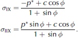
The maximum principal Stress law describes a maximum compressive principal Stress, that is σ2 ≥ –p*, where p* is the compressive Strength under biaxial compression. according to equation (4), this law can be expressed in terms of the Stress
The parameters involved in the yield curve are p*, φ and c. The two-dimensional ice strength p* can be parameterized as a function of ice thickness and compactness (e.g. Hibler, 1979):
Where P* is the three-dimensional ice Strength and C is the reduction due to compactness.
The angle of friction can be determined through the relationship (e.g. Reference NeddermanNedderman, 1992)
Where φ is the Smaller angle between the intersecting lkfs. within compacted pack ice, a typical angle of φ is about 30˚ (e.g. Reference Marko and ThomsonMarko and thomson, 1977; Reference Kwok, J.P., Shen and ShapiroKwok, 2000), resulting in a typical angle of friction of 60˚.
Measurement of the cohesion c in geophysical Scales is very rare. in most cases, it is assumed to be 0 (e.g. Reference CoonCoon, 1974; Reference smithSmith, 1983; ip and others, 1991; Reference Tremblay and MysakTremblay and mysak, 1997). however, it may be important in numerical modeling of lkfs (e.g. Reference Coon, Knoke, Echert and PritchardCoon and others, 1998; Reference Hibler and SchulsonHibler and Schulson, 2000; Reference Hopkins, Dempsey, Shen and ShapiroHopkins, 2000; Reference Hutchings, Hibler, Squire and LanghorneHutchings and Reference Hibler and SchulsonHibler, 2002). therefore keeping this parameter in the present constitutive law is appropriate. in practice, it may be related to p* by
Where n is a constant, possibly ranging between 5 and 20 according to the field observation during the Sea ice mechanics initiative (Reference Coon, Knoke, Echert and PritchardCoon and others, 1998).
The thick Solid lines in figure 2 Show the yield curve as expressed in the coordinates of the Stress invariants. for comparison, the cohesion c has been Set to 0. other Similar yield curves Shown in figure 2 are: dash-dot lines together with the thick lines connecting to –p * (ice-cream cone) (Reference CoonCoon, 1974); thin Solid curve (teardrop) (Reference RothrockRothrock, 1975);

Fig. 2. Typical yield curves used in Sea-ice dynamics in the coordinates of the Stress invariants: dash-dot lines together with the thick lines connecting to –p * (ice-cream cone) (Reference CoonCoon, 1974); thin Solid curve (teardrop) (Reference RothrockRothrock, 1975); thin Solid lines (square) (Reference Pritchard and SelvaduraiPritchard, 1981); dashed lines (Coulomb’s law) (Tremblay and Mysak, 1997); dotted lines and curve (modified Coulomb’s law) (Reference Hibler and SchulsonHibler and Schulson, 2000); and thick Solid lines (diamond) (present Study). For comparison the cohesion c takes 0 and the Slope angles are all taken from the original papers accordingly (see text for details).
Thin Solid lines (square) (Reference Pritchard and SelvaduraiPritchard, 1981); dashed lines (coulomb’s law) (Reference Tremblay and MysakTremblay and mysak, 1997); and dotted lines and curve (modified coulomb’s law) (Reference Hibler and SchulsonHibler and Schulson, 2000). all the yield curves except the teardrop applied coulomb’s law. the angles of friction are all taken from the original papers, being 35˚ (Reference CoonCoon, 1974), 90˚ (Reference Pritchard and SelvaduraiPritchard, 1981), 30˚ (Reference Tremblay and MysakTremblay and mysak, 1997), 45˚ (Reference Hibler and SchulsonHibler and Schulson, 2000) and 60˚ in the present Study.
At the intersecting point of the present yield curve, x (fig. 2), we have
This point is the demarcation between the uniaxial compression and the coulombic Shear.
In the case of constant ice-strength parameters (p *, δ and c), expressing the yield curve in terms of the Stress components σ 11, σ 22 and σ 12, we can obtain these components by Solving together the momentum equation and the yield curve equations. however, when these parameters vary with ice conditions, we must consider the evolution of the velocity and mass fields Simultaneously, as done in most dynamics models (e.g. Reference Coon, Maykut, Pritchard, Rothrock and ThorndikeCoon and others, 1974; Reference HiblerHibler, 1979).
Flow Rule
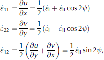
The flow rule is the equation relating the Stress tensor to the rate-of-strain tensor. Similar to what was done for the Stress, for the rate-of-strain tensor ![]() the invariants are
the invariants are
Where
Is the rate-of-strain deviator. the principal rates of Strain are
These principal rates of Strain can Similarly be obtained by turning the x-y coordinates counterclockwise with an angle of δ, where
For granular materials the lévy–mises flow rule, also known as the coaxial flow rule, is often applied (e.g. Reference NeddermanNedderman, 1992). this flow rule States that the Strain-rate and Stress deviators are proportional:
Where λ ' is a Scalarvariable. this condition leads to δ = ψ, that is, the principal Stresses and the principal rates of Strain are coaxial. the disadvantage of this flow rule, however, is that it does not provide a means to estimate the divergence. on the other hand, the normal flow rule is often applied to the Sea-ice dynamics (e.g. Reference Coon, Maykut, Pritchard, Rothrock and ThorndikeCoon and others, 1974; Reference HiblerHibler, 1979; Reference Pritchard and SelvaduraiPritchard, 1981). the normality can be expressed by
Where λ is a non-negative Scalar variable and F is the yield curve. comparing equations (16) and (17) we can See that the normal flow rule automatically possesses the coaxial property; it is therefore a Special case of the coaxial flow rule.
For the ice Stress on the yield curve of uniaxial compression, as Shown in equation (8), applying the normal flow rule leads to
This result Shows that the ice is undergoing uniaxial compressive deformation, producing ice ridges perpendicular to the compressive Stress. Such a deformation pattern is physically reasonable. therefore, we can take the normal flow rule to describe the uniaxial compressive flow.
Similarly, applying the normal flow rule to coulomb’s friction law, as Shown in equation (7), we have
In general, Such divergence is overestimated (e.g. Reference NeddermanNedderman, 1992; Reference Tremblay and MysakTremblay and mysak, 1997). as a result, the normal flow rule does not apply in this case. following Reference Balendran and Nemat-NasserBalendran and nemat-nasser (1993), an angle of dilatancy δ can be employed to replace δ, which gives
The angle of dilatancy δ here is generally less than δ. as a consequence, the normality is no longer fulfilled. in addition, as a dense Sample the compacted pack ice would normally possess a positive δ (Reference Balendran and Nemat-NasserBalendran and nemat-nasser, 1993). then a continuous dilation leads to a continuous decrease of the ice compactness and δ. when the Stress ratio σ II/σ I reaches the peak (point x in fig. 2), the critical Stress State appears, where the dilatancy becomes 0. in Such a case, δ may be parameterized along the yield curve of coulomb’s Shear Such that
Where δ m is the maximum angle of dilatancy. it may take 20˚, with 10˚ (Reference Tremblay and MysakTremblay and mysak, 1997) as a mean.
figure 3 Shows the ratios of divergence to Shear, for different yield curves and flow rules. as can be Seen, the ratios from coon’s cream cone and pritchard’s Square are rather close to that of the present Study, consisting of a uniaxial compression and Shear. the difference in these three constitutive laws lies in how much divergence would occur during Shear. tremblay and mysak’s constitutive law, as has been pointed out, takes an overall divergence when the compressive Stress is higher than –p *. rothrock’s teardrop with the normal flow rule possesses a Small divergence when σ I is low, but results in Significant convergence when σ I becomes close to –p *. hibler and Schulson’s constitutive law generally yields a Small ratio of divergence to Shear, but it tends to be quite large when σ I approaches 0 or –p *. as Suggested by equation (1), the teardrop and modified coulomb’s law hardly result in uniaxial pressure ridges, which implies that in the case of high mean compressive Stress these two constitutive laws are less effective than the others. and using a constant divergence rate in tremblay and mysak’s constitutive law does not predict compression except when the mean compressive Stress reaches –p *, which is physically unreasonable. for the constitutive laws applied by Reference CoonCoon (1974) and Reference Pritchard and SelvaduraiPritchard (1981), we know that the typical angle of friction needs to be about 60˚ and that the normal flow rule usually overestimates divergence during Shear. therefore, the present constitutive law possesses the highest capability in modeling the observed lkf and divergence patterns. further determination of the ratio of divergence to Shear can be achieved by checking the available Satellite observations (e.g. Reference Kwok, J.P., Shen and ShapiroKwok, 2000).

Fig. 3. The ratios of divergence to Shear, η = ͘εI/͘εII, for different yield curves and flow rules: (a) yield curve of ice cream cone with the normal flow rule (Reference CoonCoon, 1974); (b) teardrop yield curve with the normal flow rule (Reference RothrockRothrock, 1975); (c) Square yield curve with the normal flow rule (Reference Pritchard and SelvaduraiPritchard, 1981); (d) Coulomb’s law with the coaxial flow rule (Reference Tremblay and MysakTremblay and Mysak, 1997); (e) modified Coulomb’s law with a combined normal and non-normal flow rule (Reference Hibler and SchulsonHibler and Schulson, 2000); and (f) diamond yield curve with a combined normal and coaxial flow rule (present Study).
The flow rule on the three corners in the present constitutive law needs Some Special treatment. basically, the corner where σ I = 0 can be Seen as a pure divergence case, while the corner where σ I = –p * can be Seen as a pure convergence case. at the intersecting point x (fig. 2), the maximum Shear Stress reaches the peak, and the flow rule can be regarded as a pure Shear case. Such treatment is consistent with the classical tresca yield curve with the normal flow rule.
With the coaxial flow rule, the components of the rate of Strain can be expressed by
Where u and v are the two-dimensional ice velocity components. combining equations (15), (18)/(20) and (22) gives two equations describing the evolution of u and v, from which the velocity field can be obtained, provided the boundary conditions are given.
Concluding Remarks
A new constitutive law is presented to describe the plastic behavior of pack ice, as Shown in equations (7), (8), (16), (17), (20) and (21). the yield curve consists of coulomb’s friction law describing the in-plane Shear, and the maximum principal Stress law describing the out-of-plane uniaxial compression. for the Shear deformation, the coaxial flow rule with a parameterized dilatancy is proposed, while for the uniaxial compression the normal flow rule is Shown to be appropriate. this constitutive law is not only capable of Simulating the in-plane Shear and out-of-plane uniaxial compression, but also capable of avoiding overestimation of divergence during Shear.
A comparison of the present constitutive law with other Similar laws Shows that the present constitutive law possesses the highest capability in modeling the observed lkf and divergence patterns. this law has physical Significance in forming the pressure ridges and intersecting lkfs, resulting in a typical angle of 30˚ between the intersecting lkfs.
Acknowledgements
I am extremely grateful to m. leppäranta and two anonymous reviewers, whose comments greatly improved the manuscript. this work was partly Supported by the chinese national natural Science foundation under contract 40233032 and by the maj and tor nessling foundation of finland. the chancellor’s travel grant of the university of helsinki is also gratefully acknowledged.


