


1. Introduction
Sea ice covers a substantial part of the Arctic Ocean throughout the year and yet does not entirely separate the ocean from the atmosphere. One of its key features is the presence of leads: recurring and elongated areas of open water within the closed pack ice. Leads are characterized by a very strong exchange of heat and moisture between the relatively warm ocean and the cold winter atmosphere (e.g. Reference MaykutMaykut, 1982; Reference PerovichPerovich and others, 2011). As a result, new ice is forming within leads and thereby contributes to the seasonal sea-ice mass balance. Leads have moreover been recognized as a source of global methane emissions, which makes them a potential driver for greenhouse gases (Reference KortKort and others, 2012). Sea-ice leads and associated thin-ice areas are valuable diagnostic parameters for quantification of sea-ice drift patterns (Reference Kwok, Spreen and PangKwok and others, 2013) and long-term sea-ice variability. Hence, especially in light of the observed trends in Arctic sea-ice extent (Reference Cavalieri and ParkinsonCavalieri and Parkinson, 2012; Reference Stroeve, Serreze, Holland, Kay and MaslanikStroeve and others, 2012), and with respect to the projected future changes in the Arctic climate system, the structure and dynamics of leads represent essential parameters for global change monitoring (e.g. Reference Holland, Bitz and TremblayHolland and others, 2006; Reference KoenigkKoenigk and others, 2013). Sea-ice models generally have too coarse a resolution to simulate leads explicitly. Instead, subgrid lead fraction in global and regional sea-ice/ocean models is parameterized (e.g. Reference Timmermann, Danilov, Schröter, Böning, Sidorenko and RollenhagenTimmermann and others, 2009). Since the presence of leads has a strong effect on the atmospheric boundary layer and ocean processes, verification datasets for lead parameterizations are needed.
Monitoring of leads has been performed in previous studies using airborne and satellite sensors. Image cross-correlation techniques were applied to synthetic aperture radar (SAR) data and evaluated by Reference Fily and RothrockFily and Rothrock (1990) to identify lead opening and closing areas. Reference Key, Stone, Maslanik and EllefsenKey and others (1993) investigated the occurrence of leads by means of thermal infrared (IR) and visible satellite imagery from the Advanced Very High Resolution Radiometer (AVHRR) and Landsat. They focus on the retrieval of lead width for some image frames. In a similar manner, binary lead maps for specific Arctic regions are produced from AVHRR data by Reference Lindsay and RothrockLindsay and Rothrock (1995) using the concept of potential open water per pixel and a fixed threshold that is evaluated by comparison with visible data. A cloud mask is applied manually, which limits the spatial and temporal extent of the study. A region-growing approach for the detection of leads from airborne imagery during a field campaign is presented by Reference Tschudi, Curry and MaslanikTschudi and others (2002). Their processing depends on manual selection of seed points within leads. More recent studies address the potential of shape-constrained segmentation of ice floes (Reference Tarabalka, Brucker, Ivanoff and TiltonTarabalka and others, 2012) and the detection of leads from airborne visible imagery (Reference Onana, Kurtz, Farrell, Koenig and StudingerOnana and others, 2013) for single case studies.
A pan-Arctic lead proxy is provided by Reference Röhrs and KaleschkeRöhrs and Kaleschke (2012). They use passive microwave data to derive Arctic-wide lead concentration. The retrieval of a lead concentration in principle provides sub-pixel-scale resolution, but the microwave radiometer resolution is still too coarse to identify ˃50% of the lead area that is visible in 500 m resolution optical imagery (Reference Röhrs and KaleschkeRöhrs and Kaleschke, 2012). So far, no product exists that yields pan-Arctic lead maps at a resolution higher than 5 km2 on a daily basis. However, such a dataset would be highly valuable for the verification, assessment and parameterization of global climate models, ice drift patterns, atmosphere–ice–ocean processes and microwave satellite data (Reference Röhrs and KaleschkeRöhrs and Kaleschke, 2012; Reference Bröhan and KaleschkeBröhan and Kaleschke, 2014).
Therefore, this work aims at investigating the occurrence of sea-ice leads in the Arctic Ocean from thermal IR satellite data with 1 km2 spatial resolution. We use thermal IR data from the Moderate Resolution Imaging Spectroradiometer (MODIS) for the retrieval of pan-Arctic lead maps for January–April 2008. The choice of year is arbitrary, but we aim to provide a method that is also applicable to longer time series. Here we focus on the identification of leads and the implementation of a novel filter technique to avoid cloud artifacts in the daily maps. This approach advances the potential to retrieve daily lead maps operationally from satellite data at a resolution of 1 km2.
We first provide an overview of the data used and the methods applied to segment leads out of thermal IR imagery. We then describe insufficiencies in the maps obtained due to cloud effects, and propose a new technique, namely a fuzzy cloud artifact filter, to filter out the resulting misclassified leads. In Section 3.3 we tune the filter using manually selected case studies and determine the obtained filter performance. Subsequently, we show monthly aggregates of the resulting daily lead maps for January–April 2008. Finally, we discuss the remaining shortcomings of, and the future potential for improvements to, the suggested technique.
2. Data and Methods
2.1. Satellite data
MODIS satellite data are used in this study. MODIS is an instrument on board the two polar orbiting satellites Terra and Aqua, which are part of NASA’s Earth Observing System (EOS). Terra MODIS and Aqua MODIS view the entire Earth’s surface every 1-2 days, acquiring data in 36 discrete spectral bands from the optical to the thermal IR wavelength region. The swath width of MODIS is 2330 km. Continuous measurements are combined to so-called ‘tiles’ after every 5 min of acquisition, resulting in an array with 2030 (‘along-swath’)x1354 (‘across-swath’) gridpoints. Two MODIS products are used in this study:
-
1. The MODIS MOD29/MYD29 product (Reference Riggs, Hall and SalomonsonRiggs and others, 2006; Reference Hall and RiggsHall and Riggs, 2007) provides ice surface temperatures with an accuracy of ±1.6 K and a geometric resolution of 1 km2 at nadir. MOD29/MYD29 ice surface temperatures are obtained from the US National Snow and Ice Data Center (http://n5eil01u.ecs.nsidc.org/SAN/). The MODIS cloud mask (MOD35) is in the product; however, the cloud-mask algorithm has difficulties in identifying sea smoke and thin low clouds (Reference AckermanAckerman and others, 2006), especially during the polar night, which eventually results in high ice surface temperatures that are not attributed to real surface features. We downloaded all available swaths from the MOD29/MYD29 dataset that cover the region north of 658 N. This preselection was carried out using the metadata available for each MODIS swath.
-
2. The MODIS MOD02 data contain calibrated at-aperture radiances for all 36 bands. MOD02 data were acquired from the Level 1 and Atmosphere Archive and Distribution System (LAADS) at the NASA Goddard Space Flight Center (http://ladsweb.nascom.nasa.gov/). The array acquired in channel 2 (841-876 nm) is extracted from the MOD02 dataset. Channel 2 provides a resolution of 250 m x 250 m and hence serves as a useful reference for validation of segmentation techniques that are applied to the thermal IR data.
2.2. Lead segmentation
Leads (thin ice and open water) are represented by negative brightness anomalies (Fig. 1a) and exhibit a positive surface temperature anomaly (∆T s) compared with the regional surface temperature distribution (Fig. 1b) during winter when the surface temperatures of thick ice are well below the freezing point of sea water. However, ∆Ts values are not representative for any surface classes if no global (scene-independent) tie point for normalization is used. This would motivate the use of the potential open-water parameter (Reference Lindsay and RothrockLindsay and Rothrock, 1995; Reference Drüe and HeinemannDrüe and Heinemann, 2004), which essentially represents a physically based normalization of ∆Ts with the freezing temperature of open water. However, here we aim to segment leads swath-wise with a binary approach, for the reasons itemized in Section 3. In this regard, a cross-scene normalization is not required. Moreover, the assumption of a tie point at -1.88C suffers essentially from the ±1.68C accuracy of MODIS surface temperatures (Reference Hall and RiggsHall and Riggs, 2007). Hence, we present different segmentation techniques to separate leads from sea ice based on ∆T s maps. ∆Ts per pixel is calculated as the deviation from the median in a box of 51 x 51 gridpoints. This box size is sufficient to exceed the scale of leads, while keeping the effect of regional surface temperature gradients due to differences in atmospheric conditions small. Swath-scale temperature gradients are removed with this approach (Fig. 1c). Provided that the surface temperature anomaly over thick ice follows a normal distribution with a mean of zero, leads introduce an amplification of the right-hand tail in the ∆T s histogram (Fig. 1d). The onset of this effect is thus detected and defined as a threshold for binary lead segmentation.
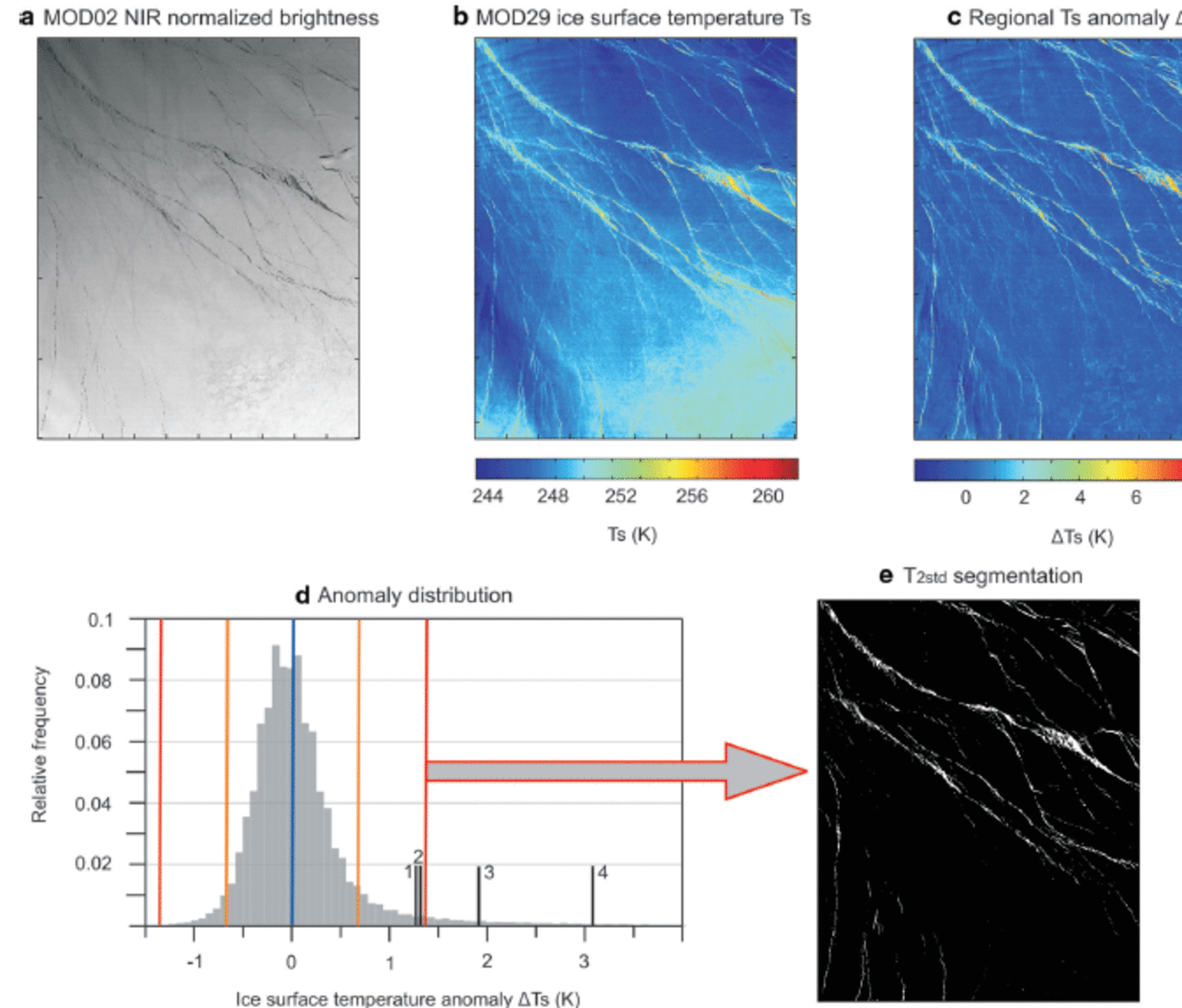
Fig. 1. MODIS swath data from 9 April 2008, 01.35 UTC, central Beaufort Sea: (a) NIR normalized brightness (MOD02, 250 m x 250 m), 2500 x 2000 gridpoints; (b) ice surface temperature product (MOD29, 1 km x 1 km), 625 x 500 gridpoints; (c) local ice surface temperature anomalies based on the median temperature of the 51 x 51 surrounding box; (d) histogram of surface temperature anomalies with mean (blue), STD (orange) and STD*2 (red) indicated and black lines representing non-parameterized thresholds (1: T Otsu; 2: T iterative; 3: T min error; 4: T max_entropy); and (e) segmentation result with ∆T s threshold = T 2std.
In a first approach, we determine the threshold at the mean surface temperature anomaly + 2 standard deviations (T2std; Fig. 1e). Additionally, we tested a set of non-parameterized global threshold techniques: iterative selection (T iterative; Reference Ridler and CalvardRidler and Calvard, 1978), Otsu’s threshold (T Otsu; Reference OtsuOtsu, 1979), minimum error threshold (Tmin_e rror ; Reference Kittler and IllingworthKittler and Illingworth, 1986) and maximum entropy threshold (T maxentropy; Reference ParkerParker, 2011). All these methods aim at an optimal separation of two brightness classes within a given histogram of gray values using different metrics and rules of iteration to evaluate their separation. We further use an adaptive threshold (minimaxAT) approach, which is carried out by an iterative gradient descent with exact line search techniques (Reference Saha and RaySaha and Ray, 2009). Additionally, an active contours model (ChanVese; Reference Chan and VeseChan and Vese, 2001) is applied that implements techniques of curve evolution to detect objects whose boundaries are not necessarily defined by gradient. Finally, we test the performance of a region-growing procedure (regionGrow; Reference Gonzalez, Woods and EddinsGonzalez and others, 2004) since this represents an established method in image segmentation where a decision is provided as to whether pixel neighbors of manually selected seed points should be added to the seed region. For a detailed description of the methods the reader is referred to the literature provided. We tested all these methods to evaluate potential advantages of any technique for lead recognition. It is necessary to consider that region-growing techniques require the manual selection of seed points and that active-contour models are computationally intense, which makes them both questionable candidates for operational use.
The binary segmentation for an image subset is given in Figure 2 (1-8). The presence of leads with different widths is indicated in the near-IR (NIR) MOD02 image (Fig. 2a). The binary results show that significant leads are easily recognized by all of the applied techniques; however, they differ in their ability to detect narrow leads and leads with thin ice where the regional temperature anomaly within the 1 km x 1 km box is less significant.

Fig. 2. MODIS swath data from 9 April 2008, 01.35 UTC, central Beaufort Sea (subset): (a) NIR normalized brightness (MOD02, 250m X 250 m), 450 X 350 gridpoints; (b) segmentation results based on ΔTs (1km X 1 km) (1: Titerative; 2: T2std; 3: TOtsu; 4: Tmin_error; 5: Tmax_entropy; 6: TminimaxAT; 7: TChanVese; 8: TregionGrow).
2.3. Segmentation validation
Segmentation performance metrics are calculated using the normalized brightness values derived from MOD02 data. We use manually selected cloud-free images from the MOD02 NIR channel as a reference for validation of the surface-temperature-based segmentation. Provided that leads are characterized by a negative brightness anomaly, we assume that pixels with a normalized brightness exceeding the 75th percentile of the respective swath cannot be leads, while pixels with a normalized brightness undershooting the 15th percentile cannot be thick sea ice. With this, the fraction of lead objects as identified from the thermal IR data covering areas where the normalized channel 2 brightness is larger than the 75th percentile are regarded as misclassified leads, while the fraction of detected sea ice covering brightness values below the 15th percentile are regarded as unclassified leads. The probability of lead detection (PLD) and probability of background (sea-ice) detection (PBD) are used as statistical performance indices for the applied segmentation methods: PLD denotes the fraction of correctly identified leads (L c) relative to the total fraction of leads (L c plus falsely classified background B f; Eqn (1)), while PBD gives the rate of correctly identified background B c over the total background (B c plus falsely classified objects L f; Eqn (2)).
Both metrics are shown in Figure 3 and give insight into the individual performances of the different techniques. It is shown that the three non-parameterized global threshold techniques provide similar performance values (PLD). The background (sea-ice) segmentation, hence PBD, appears to be substantially lower when T 2std is used, which is manifested by the lower mean and larger standard deviation. T min_error and T max_entropy are both characterized by lower performance compared with the first three techniques. The adaptive threshold and shape-based segmentation techniques (minimaxAT, ChanVese, regionGrow) are less reliable for operational use with multiple swaths, which we conclude from their low average PLD values (Fig. 3). Finally, we choose iterative for the subsequent processing steps, since it shows the highest performance of the methods tested.
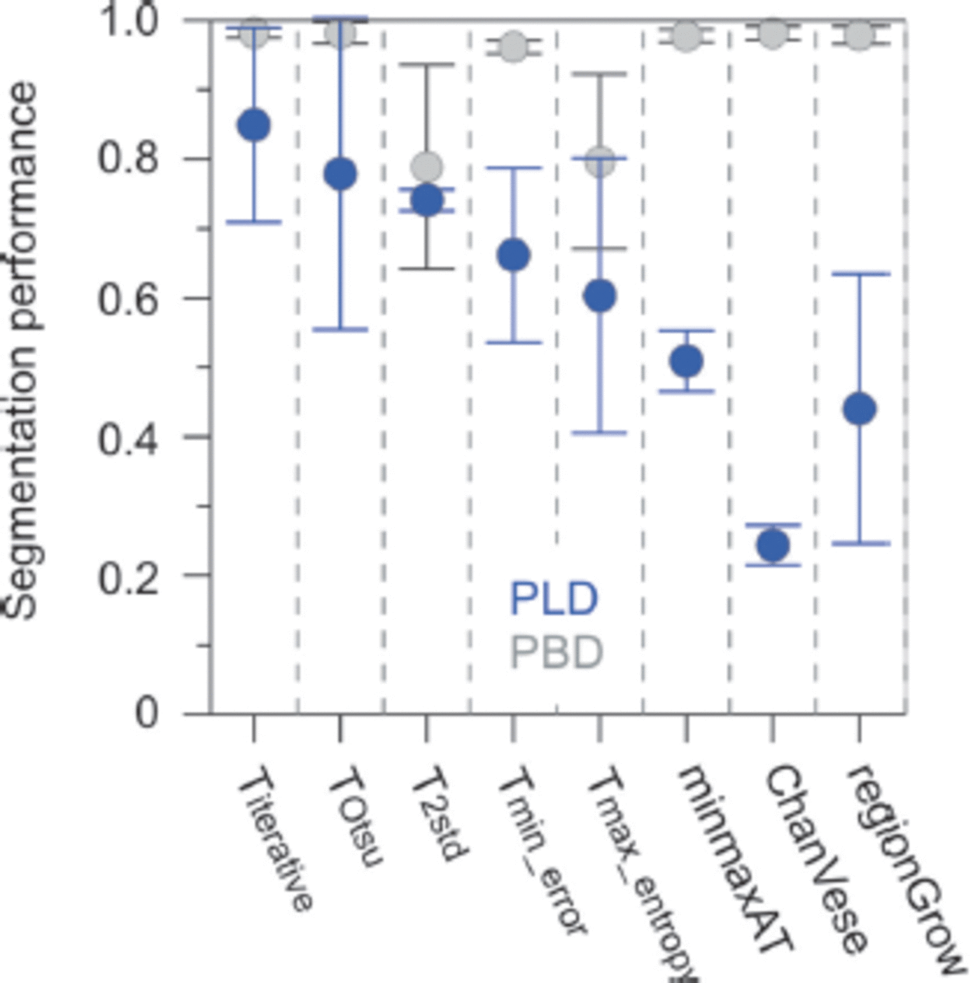
Fig. 3. Lead and background segmentation performances as expressed by probability of lead detection (PLD, blue) and probability of background detection (PBD, gray) for different segmentation techniques. Mean values and standard deviations as inferred from five arbitrarily chosen MODIS tiles, where NIR normalized brightness anomalies (MOD02) were compared with the binary segmentation results from the regional surface temperature anomalies (MOD29).
2.4. Daily lead composites
For each tile, MODIS ice surface temperature data (MOD29/ MYD29) are first interpolated to a pan-Arctic grid with a resolution of 1 km2. Subsequently, ∆T s is calculated and lead segmentation is performed using the iterative threshold technique (T iterative). Thereby a binary lead map is derived with remaining cloud pixels being flagged separately. Daily composites are produced by filling the pan-Arctic map with consecutive binary lead maps, applying the rule that clouds (NaN flag) are replaced by sea ice (false) and, if applicable, sea ice is replaced by a lead (true) (Fig. 4). The daily composite is also saved as a stack, providing the number of leads found per pixel and day, for later use as a persistence indicator (see Section 3.1).

Fig. 4. (a) Binary lead (red)/sea-ice (black) map. Daily composite from binary swaths for 16 March 2008 with remaining cloud pixels shown in white. (b) Accumulator map indicating number of lead hits per pixel and day. Subsets of (a) and (b) give examples of the presence of cloud artifacts.
As leads are derived in binary (no information on concentration), it is necessary to bear in mind that a segmented pixel reveals significant lead activity within its area rather than representing this lead with its full width. As stated above, the binary approach has the advantage that no cross-image tie point is necessary. The composite in Figure 4 shows the presence of extended linear features in different regions: fast ice and flaw polynyas in the Laptev Sea, as well as broad areas that indicate the presence of significant and extended small-scale lead activity. It is apparent that the area of the remaining cloud pixels is becoming very small, if the compositing rules described above are applied. However, an analysis of subsequent segmentation maps reveals that some segmented objects are very short-lived or are moving fast within a short time. This behavior indicates that the segmentation is subject to artifacts that arise from unidentified clouds and that need to be removed in subsequent processing steps.
2.5. Cloud artifacts
The MODIS cloud mask has deficiencies in identifying low and thin clouds over sea ice as well as sea smoke, especially when no reflected sunlight is available (Reference AckermanAckerman and others, 2006; Reference Riggs, Hall and SalomonsonRiggs and others, 2006). This eventually causes high surface temperatures that are in fact not attributed to surface features. A useful validation of the cloud mask over large spatial scales is not possible since no valuable reference data exist. The processing of daily lead composites as described above hence produces cloud artifacts in the obtained binary lead maps due to erroneously high surface temperatures.
An example of this is given in Figure 4. With regard to their structure and translation speed (from image sequences), the classified objects are easily identified as cloud artifacts by an experienced observer. However, as shown in Figure 4a, the anomaly is recognized as a lead by the segmentation algorithm. Since cloud patterns can be identified by their drift speed, a filter was implemented using optical flow and maximum cross-correlation techniques. However, the discontinuity in the 6 hourly composites is too pronounced to derive flow fields and thereby identify artifacts. Instead, the transient character of lead objects, in combination with the vague and imprecise character of the cloud mask quality, motivated the use of fuzzy logic techniques to implement a filter for cloud artifacts. As stated by Reference ZadehZadeh (1965), the use of imprecise information is beneficial in knowledge-based systems as the advantage of reduced system complexity can be utilized. Here, a Mamdani-based fuzzy interference model was created as a filter for separating true leads from cloud artifacts. This implementation is hereafter referred to as the Fuzzy Cloud Artifact Filter (FCAF). It is first necessary to define suitable indicators that allow us to distinguish between leads and artifacts. In principle, independent data from different sensors would be most beneficial in that sense; however, for this study no additional data were available with a comparable resolution. Hence, we derive different object and pixel properties from the same dataset using temporal and spatial concepts as described below.
3. FCAF
3.1. FCAF design
Three main object features were determined – two for temporal and one for spatial object properties – which can be used as an input to the fuzzy interference system and allow differentiation between leads and cloud artifacts:
1. The pixel persistence (PP) is defined as the number of true values (leads) within the daily pixel stack. PP is normalized over the stack size at each gridpoint. The stack size is different at every gridpoint and consists of as many layers of the cloud-free swath data as were available per day. This normalization also avoids a potential bias due to higher swath frequency at higher latitudes. The use of PP is motivated by the fact that fast-moving clouds will have a low PP; its deficiency lies in the fact that leads with short duration or strong drift will be discarded.
2. The object persistence (OP) accounts for the fact that drift might cause a low PP at one gridpoint. The OP of any pixel is derived by assigning the maximum PP value of the same binary object within a box of 10 x 10 pixels to each pixel. OP thereby mitigates the loss of short-lived leads. The limited search radius for OP values avoids overestimation of OP in overlapping and large objects.
3. Object solidity (OS) represents a morphological object feature specifying the ratio between the area of the surrounding rectangular box of an object and the object area itself. Its use is based on the concept that leads are characterized as predominantly linear features and hence provide high degrees of eccentricity. Here the circular OS (circle area instead of box area) is calculated to make solidity independent of the object orientation within the matrix. The inverse is used to associate high values with high degrees of eccentricity. OS is calculated for each 6 hourly map to avoid too much object overlapping, and is then integrated to an accumulated daily OS map. OS is useful to avoid discarding small and short-lived leads that show pronounced eccentricity.
Subsequently, different fuzzy sets are defined for each input variable (PP, OP, OS), with each set representing a different system configuration. Linguistic terms like ‘low’, ‘average’ or ‘high’ can be associated with each degree of membership and are used to formulate logical rules that connect each grid element with its current state to the system response. A subset of a feature set describing a pixel’s state would look like
with the system state (P) at positions x and y described by three features and their degree of fulfillment. The nonlinear system response is calculated from single rule outputs and respective weights. A vector of input values creates a specific system response, i.e. a membership value for the lead class. The regional variability of the three state variables for 16 March 2008 is shown in Figure 5. A pronounced regional variability is found in all these variables.
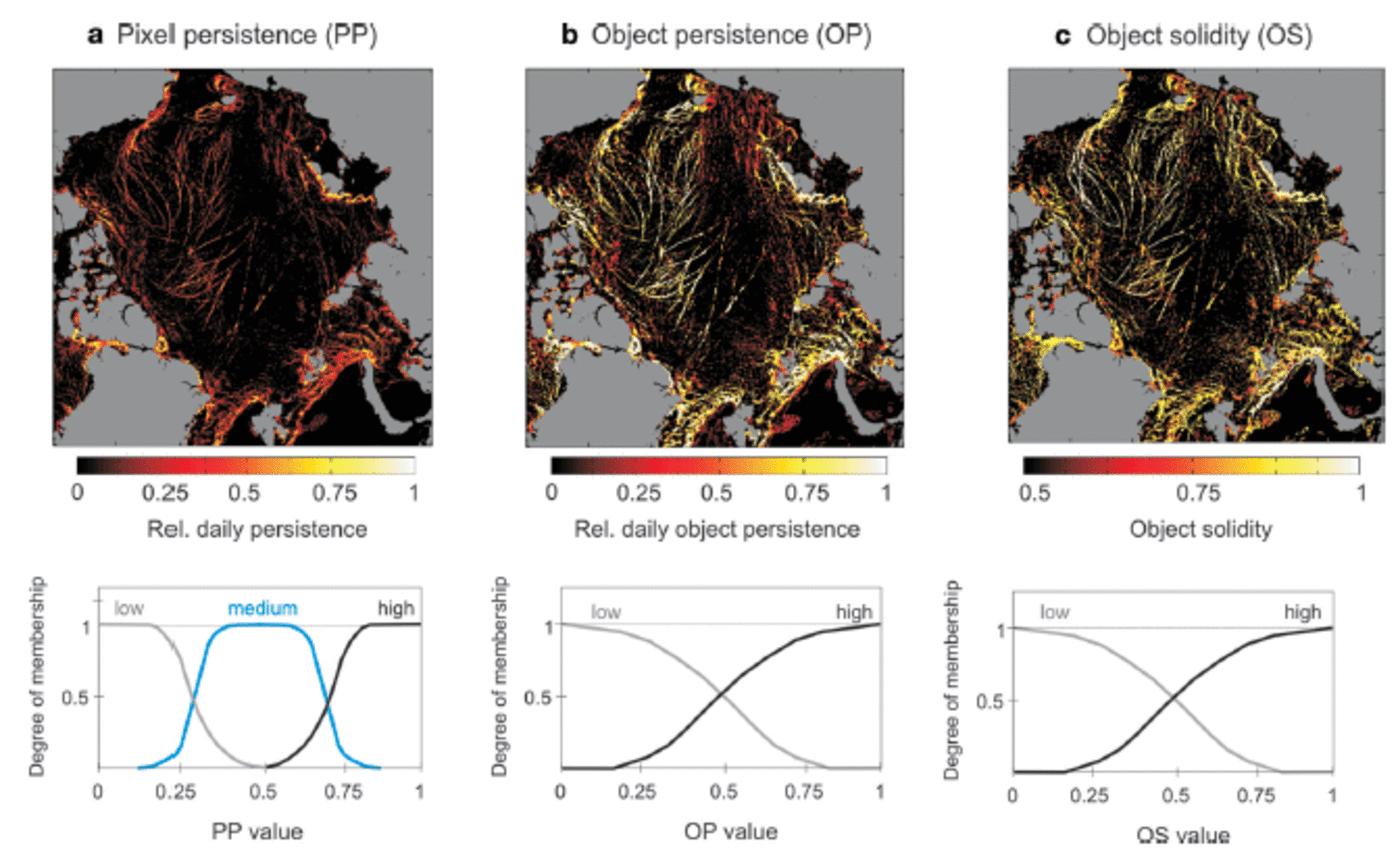
Fig. 5. (a) Pixel persistence (PP), (b) object persistence (OP) and (c) object solidity (OS) values for 16 March 2008, each with its associated membership functions (lower panels).
3.2. FCAF membership functions and rules
A membership function describes the degree of membership of a given pixel value to predefined categorical states. For example, PP is assigned three membership functions (MF): low, medium and high. Thereby, PP is exclusively low (degree of membership to the MF low is 1) for PP values ˂0.15. The degree of membership to the MF low is consequently decreasing with increasing PP value, while the following MF (medium and, with further increasing PP, high) are iteratively gaining power (Fig. 5a, lower panel). The OP and OS memberships are assigned two Gaussian functions for memberships to low and high (Fig. 5b and c, lower panels). In the same manner, the system response is prescribed in the form of the degree of membership to an MF islead (yes) and islead (no).
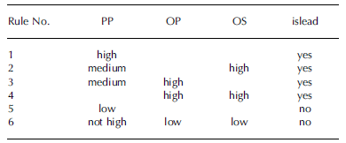
The relative daily PP is considered the strongest criterion for a lead detection. A pixel with a PP value equal to 1 (lead is present in all available stack data) is always assigned a lead (rule 1). With decreasing PP, the fuzziness of the segmentation increases and hence the secondary object features OP and OS apply in additional rules (see Table 1). For example, a PP with a high degree of membership to MF medium causes the FCAF to recognize a lead only if OP or OS show pronounced degrees of membership to high MFs (rules 2 and 3). Rule 4 permits smaller leads with low PP to pass the filter only when high OP and OS values are found. Rules 5 and 6 represent explicit formulations of the criteria used to discard a lead. It is necessary to bear in mind that implicit filtering also takes place when rules 1–4 cause a low system response. This response (islead), which represents the decision whether the segmented object represents a true lead or not, is returned as the degree of membership to two Gaussian functions (yes or no) in similar manner to the OS input.
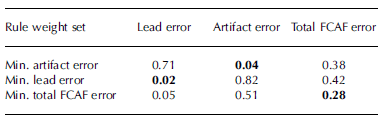
Table 1. FCAF rules and weight for minimum total FCAF error (see Section 3.3)
3.3. FCAF validation and tuning
If all the rule weights are initialized with 1, the system creates an output that is hardly verified in terms of quality. An objective rule weight optimization was addressed by the following steps. First, sub-scenes from different case studies are chosen that contain two classes: leads and cloud artifacts. The decision whether one of the two classes really applies is made based on background knowledge of the surface features, as well as on detailed analysis of the temporal evolution of the object in question based on image sequences. Next, two maps are created, one containing a subset of pixels that are confidently determined as artifacts and another showing exclusively real leads (Fig. 6, red areas on left). These two areas in total represent the reference area for one case study.

Fig. 6. Weight optimization scheme. Manually selected ground truth maps are compared to fuzzy outputs during 500 iterations with randomly changing rule weights.
Subsequently, the fuzzy system is run at 500 iterations, with weights assigned randomly at each iteration step. The respective output is then compared with the manual selection, with two error indicators combined to the total FCAF error (Fig. 6). The set of rule weights can now be chosen according to different performance targets: either artifact, lead or the total FCAF error (average of lead and artifact error) can be minimized. The first comes at the cost of true leads being discarded while the filter is more restrictive. The second option allows the maximum fraction of lead pixels to pass the filter, while also more artifacts are taken over in the filtered result. The total FCAF error minimization aims to keep the total error as small as possible.
The obtained error values are given in Table 2. Rule weights can be defined such that artifact and lead errors can be minimized. If the focus is on artifact removal, the total FCAF error is 38%. If a correct lead identification is prioritized (only 2% of true leads are falsely discarded in the validation subsets), the total FCAF error is 42%.
If the total FCAF error is to be kept small, 5% of leads are erroneously filtered out and 51% of artifacts are missed, which amounts to a total FCAF error of 28%, or a performance of 72%. Hence, here we use this FCAF rule weight set for any further processing, keeping these performance values in mind.
The result of the FCAF application for a daily composite is given in Figure 7. Depending on the choice of weight sets, the fraction of filtered objects ranges from 93% (artifact error minimization; Fig. 7a) to 59% (lead error minimization; Fig. 7c). Minimizing the combined error causes 77% of potential lead pixels to be removed (Fig. 7b). The main difference between the outputs of the three different filter configurations is found in the presence of small and thin objects. The most prominent lead structures and the location of flaw polynyas are preserved even when the artifact error is minimized (Fig. 7a). It is clear that a large fraction of the segmented objects is filtered out by the use of the FCAF. On average 82% of the segmented pixels are removed by the FCAF for 1 January to 30 April 2008.

Fig. 7. FCAF results for 16 March 2008 showing weight set applied for (a) minimum artifact error, (b) minimum total FCAF error and (c) minimum lead error.
4. Discussion and Outlook
The FCAF parameterization is subject to a trade-off in acceptable errors (Table 2). However, the difference between the artifact and lead error minimization maps (Fig. 7a and c) could be utilized to derive a confidence flag. Lead identification with differing confidence levels motivates the preparation of an aggregated product, i.e. 3 day, weekly or monthly lead maps where areas with significant lead activity emerge in a more distinct manner than areas with unclear segmentation.
Table 2. Weight set and associated FCAF errors. Numbers indicate areal fraction of erroneous filtering. Bold numbers indicate the minimum error values that could be obtained for each of the three weight sets
Small leads with a minor effect on the 1 km x 1 km surface temperature anomaly will be missed by our segmentation approach. An empirical lead width distribution would be beneficial to quantify the effect of this scale gap and to estimate the smallest lead fraction required within a gridcell of thermal IR imagery for the presented approach to work.
We present lead frequencies per gridpoint and month in Figure 8. In the same manner, weekly maps can be processed. A monthly aggregate as shown here already gives a good indication of the seasonal evolution of divergence patterns, with the Beaufort Sea showing the most significant lead activity in the study period. Particularly in January, large and pronounced leads are present in this region, while extended leads occur with increasing frequency in the central Arctic and north Greenland in March and April. The presence of flaw polynyas is well reproduced by the monthly maps. This indicates the potential use of these maps for retrieval of the monthly fast-ice extent. Daily maps were also compared with the results of the technique described by Reference Röhrs and KaleschkeRohrs and Kaleschke (2012), which yielded a high congruency for large and extended leads in the daily maps. We intend to use our method with further elaborations to provide daily lead maps for the entire MODIS period, providing sea-ice surface temperature data from 2000 onwards. We see great potential in combining the described segmentation product from MODIS data within an enhanced FCAF system with the microwave lead product of Reference Röhrs and KaleschkeRöhrs and Kaleschke (2012) and with active microwave data (e.g. Reference Early and LongEarly and Long, 2001) to allow more independent data to determine the artifact filter response. Additionally, high-resolution SAR data for case studies will be useful to achieve improved FCAF tuning when new parameters are introduced.
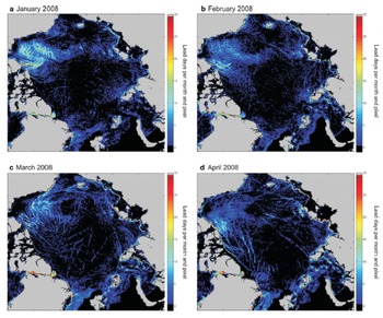
Fig. 8. Monthly lead frequencies (lead days per month) for (a) January, (b) February, (c) March and (d) April 2008 derived from daily FCAF outputs.
5. Conclusions
A non-parameterized global threshold method was validated and applied to derive binary lead maps from regional surface temperature anomalies derived from the MODIS ice surface temperature product. Swath-based binary maps were subsequently combined into daily pan-Arctic composites for January–April 2008. Results reveal the presence of cloud artifacts in the lead identification, which is caused by ambiguities in the MODIS cloud mask. To mitigate these artifacts we implemented a fuzzy filter system that employs temporal and spatial object characteristics to distinguish between physical leads and artifacts. The filter was tuned to keep the combined error (lead and artifact misclassification) at a minimum, which results in 5% of missed leads and 5 1% of non-recognized artifacts. The results obtained lend themselves to monitoring of seasonal sea-ice divergence patterns. For follow-on studies, we recommend the use of satellite-derived microwave data in the discrimination process to significantly improve the filter performance. We aim to use this technique to compute daily wintertime pan-Arctic lead maps for the entire MODIS data archive (2000 onwards).
Acknowledgements
This study was funded by the German Ministry for Education and Research (Bundesministerium für Bildung und Forschung, BMBF) under grant 03G0833D, and is part of the German–Russian Transdrift project. Valuable comments from P. Gemmar (Hochschule Trier), Stefan Kern and two reviewers are gratefully acknowledged.


