


1. Introduction
The mass balance of Sea ice is one of the key parameters in Studies of the cryosphere. accurate knowledge of this quantity is of fundamental importance for climate and ocean models as well as for quantifying past and future changes. Satellite remote Sensing can be used to estimate the lateral dimension of the Sea-ice cover. however, ice thickness cannot be derived directly from Satellite data, So estimates of the mass balance are difficult. as Sea ice is found in remote regions, field campaigns are difficult and costly. in addition, ground-based thickness measurements can only be carried out on local and regional Scales. indirect methods to determine the mass balance of Sea ice from remote Sensing are therefore crucial.
This Study presents an analysis of the Surface roughness relative to level-ice thickness. the level-ice thickness rather than the mean thickness is analyzed, as it represents the prevailing thickness along a profile, assuming that for Sufficiently long profiles the length of the level-ice Sections in the profile is greater than the length of the deformed-ice Sections. we take this value as representative of different ice types as defined by the World meteorological organization’s Sea-ice nomenclature (wmo, 1989). level-ice thickness is estimated from the observed modal thickness. roughness, in our context, is determined by undulations of Surface height over the entire profile, comprising both Smaller undulations on level ice and deformation features Such as ridges and rubble. the question is addressed whether different ice types can be discriminated in an analysis of the Surface roughness properties. Reference GoffGoff (1995) derived a method for Stochastic modelling of Sea-ice draft. he generated Synthetic draft profiles from a Set of Statistical parameters estimated from upward-looking Submarine Sonar data and compared these profiles to observed data. we take the positive results of his comparison as a motivation to investigate whether the roughness properties of Surface profiles, described by a Set of Statistical parameters, are characteristic for different ice types. the work focuses on the roughness of the top Side only, as this property affects measurements from air- and Space-borne Sensors Such as radar and laser.
2. Data
To derive the classification algorithm, data from the cruise ark xix of r/v Polarstern to the fram Strait and barents Sea, arctic ocean, in march–april 2003 were used. available data consist of Surface elevation and thickness profiles. the ice-thickness profiles were obtained by electromagnetic induction Sounding, the Surface profiles by laser altimetry. both Sensors were mounted on the Same platform, the ‘hem bird’, which was towed over the ice by a helicopter at an altitude of 10–15m above the Surface. ice-thickness data were acquired with an accuracy of 0.1 m and a point Spacing of 3–4 m. the Surface elevation profiles were measured with a riegl ld90-3100hs laser altimeter (905nm wavelength) with an accuracy of 3 cm and a point Spacing of 0.3–0.4 m. to remove the effect of altitude variation in the laser data due to the aircraft motion, the raw laser data were processed using a combination of high- and low-pass filters (Reference HiblerHibler, 1972), with high-pass cut-off frequency 1/40m–1. note that the resulting Surface elevation profiles are not identical to the ice freeboard, but measured relative to a reference-level Set by the processing Scheme. the reference level roughly follows the level-ice Surface. only flight profiles for which thickness and Surface elevation data were acquired Simultaneously were included in the analysis.
3. Roughness Parameters
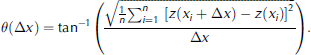
To describe Surface roughness, a number of different parameters are in use. analyses of Sea-ice roughness have been carried out in the past by, for example, Reference Rothrock and ThorndikeRothrock and thorndike (1980), Reference Bishop and ChellisBishop and chellis (1989), Reference Lewis, Leppäranta and GranbergLewis and others (1993), Reference GoffGoff (1995) and Reference ManninenManninen (1997). Several mathematical roughness characteristics used for the analysis
Of geological terrain are also described in Reference DierkingDierking (1999) and Reference Shepard, Campbell, Bulmer, Farr, Gaddis and PlautShepard and others (2001). however, unlike geological Surfaces Such as lava, the Sea-ice Surface comprises Stretches of level ice, as well as distinct vertical deformation features Such as pressure ridges. among the most frequently used parameters are the mean profile height, the Standard deviation of the profile elevation about the mean (rms height) and the autocorrelation length. another commonly used parameter is the empirical rms Slope, which measures the mean Slope angle between profile points z(x) Separated by a distance Δx (Reference Shepard, Campbell, Bulmer, Farr, Gaddis and PlautShepard and others, 2001):
Reference GoffGoff (1995) proposes to use the Skewness as an indicator of non-gaussian properties of the Surface. here, we also investigate the kurtosis, which is indicative of the properties of the peak of the distribution (for a definition, See Reference Abramowitz and StegunAbramowitz and Stegun, 1972, def. 26.1.18). another approach uses offset and Slope of the Surface’s power Spectrum to describe the roughness. however, as pointed out by Reference Bishop and ChellisBishop and chellis (1989), the asymptotic properties of the Spectrum are difficult to determine.
If the Surface Shape can be assumed to be a realization of a Stationary random process, empirical mean and Standard deviation are estimators of its true mean and Standard deviation. they take constant values and characterize the Surface regardless of the profile length. however, Several authors have Stressed the fact that the roughness of natural Surfaces is only poorly modelled by a Stationary process (e.g. Reference Sayles and ThomasSayles and thomas, 1978). instead, investigations of roughness Spectra of natural Surfaces have indicated power-law behaviour. in this case, mean height, Standard deviation and autocorrelation length cannot be used as estimates of the true values. they are not constant, but depend on the profile length and thus cannot be used to compare profiles across different length Scales.
A parameter that has been used by numerous authors to characterize the roughness of non-stationary Surfaces is the fractal dimension (Reference Rothrock and ThorndikeRothrock and thorndike, 1980; Reference Bishop and ChellisBishop and chellis, 1989; Reference Key and MclarenKey and mclaren, 1991; Reference Barabasi and StanleyBarabasi and Stanley, 1995). it describes the Scaling behaviour of a profile or Surface. for a Self-affine profile z=z(x), the height increments Scale with lag Δx according to
(angled brackets denote expected value). the Scaling parameter H is the hurst exponent, which in case of profiles is related to the fractal dimension d f by d f = 2–H. for ideal fractals, equation (1) is valid over the whole range of lags Δx. natural Surfaces, however, often display fractal properties only over a Specific length Scale (Reference Bishop and ChellisBishop and chellis, 1989; Reference DierkingDierking, 1999). on Scales larger than a certain cut-off, the Surface may Still be characterized as a realization of a Stationary random process.
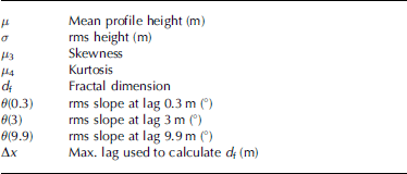
To capture the characteristics of profiles that may display fractal behaviour on one Scale, but appear to have properties of Stationary random processes on another Scale, this Study is based on parameters Suitable for Stationary random profiles as well as the fractal dimension. these parameters are listed in table 1.
Table 1. Roughness parameters
4. Classification OF Surface Profiles
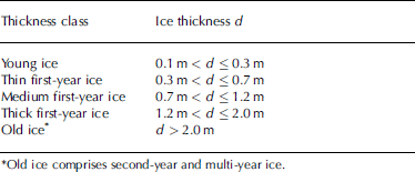
Firstly, all profiles were divided into Sections of equal length. for each profile Section, the modal ice thickness was calculated from the electromagnetic (em) data as an indicator for the level-ice thickness of that profile. the modal thickness was then used to assign the profile Sections to five ice classes according to the World meteorological organization’s Sea-ice nomenclature (wmo, 1989) Summarized in table 2.
Table 2. Wmo ice-thickness classes
Next, the roughness of the corresponding Surface profiles was analyzed. examples of laser Surface profiles for each thickness class are displayed in figure 1. for each profile, the parameters from table 1 were calculated. each profile is thus represented by a point p in nine-dimensional parameter Space. the parameter Space is partitioned into five regions Ωi (i=1,...,5) representing the five thickness classes, and an element is classified as belonging to class ωi if its corresponding parameter vector p lies in region Ωi .

Fig. 1. Examples of Surface profiles from different ice-thickness classes.
For classification of the profiles, the k-nearest-neighbour method was chosen. it is distribution-free, i.e. does not make a priori assumptions about the probability distributions of the data. the k-nearest-neighbour method is a Supervised classification procedure and therefore requires a Set of training data, for which the group assignments are known. a hypersphere is considered, centred on the element to be classified. it is chosen Such that it contains exactly k elements with known group assignments. from these, k 1 belong to class ω 1, k 2 to class ω 2, etc. the classification rule then States (Reference HandHand, 1981) that the element is assigned to class ωi if
I.e. it is assigned to whichever class most of the elements within the hypersphere belong to. here, k was chosen to be equal to the Smallest integer where n is the total number of points in the training Sample (Reference HandHand, 1981).
4.1. Performance of the classification
To assess the performance of the classification rule, the allocation error was calculated as the proportion of misallocated elements using a dataset with known group assignments. the data matrix was divided into a training Set and a test Set. the training Set was used for calculation of nearest neighbours. each element from the test Set was allocated to one of the groups as described above, and the allocation error was obtained as the proportion of misclassified elements.
As the allocation error depends on the particular choice of training and test Set, the procedure was repeated 1000 times, each time randomly drawing a training and a test Set. the division into training and test Set was Such that the training Set always contained 80% of the elements.
To assess the dependence of the classification method on the length of the Surface profiles, calculations were carried out for profile lengths of 2, 5, 8, 10 and 15 km.
4.2. Variable Selection
An important point concerns the Selection of classification variables used for discrimination between the groups. as explained above, the different parameters reflect different characteristics of the profiles. it might therefore be expected that the parameters also differ regarding their performance as classification variables. it is possible that two parameters, when used by themselves, are not very good discriminators. however, the classification performance may improve considerably when both parameters are used in combination. on the other hand, the notion that each new variable can only improve the classification is not generally true (Reference HandHand, 1981). the question which combination of the parameters to choose as classification variables therefore requires careful examination.
In this work, the parameters were chosen following a Strategy of forward Selection (Reference HandHand, 1981; Reference KrzanowskiKrzanowski, 1993), which was applied to the training Set. in the first Step, all variables were analyzed in turn to find the one that would lead to the Smallest allocation error. (the allocation error in this context was estimated by cross-validation of the training Set (e.g. Reference LachenbruchLachenbruch, 1975; hand, 1981; krzanowski, 1993).) the Single ‘best’ variable was retained, and in the next Step the allocation error was calculated for this variable in combination with each of the remaining variables. again, the pair with the Smallest allocation error was retained and the procedure was repeated for that pair combined with a third variable and So on, resulting in a list of allocation errors for ‘best combinations’ of 1, 2, . . . , 9 parameters. from this list, the combination with the Smallest overall allocation error was chosen as the final Set of classification variables, which was then used in the classification of the test Set.
As the allocation procedure was repeated 1000 times, different Sets of classification parameters were obtained. the properties and the distribution of these various combinations are discussed in Section 5.1. the results presented next, on the other hand, were obtained by averaging the allocation errors from the 1000 runs, regardless of the particular combination of classifiers used in each run.
5. Results
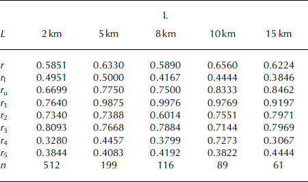
Results for the allocation errors obtained in 1000 runs are Summarized in table 3. the table also displays the within-group error rates r 1–r 5 for the five thickness classes, which are the fractions of misallocated elements from each thickness class. the mean allocation error was 58–66%, well below the value of 80% that would result if the probability of assigning an element to a particular group were identical for all groups. the Smallest allocation error was obtained for profile length L = 2 km. the within-group allocation errors for thickness classes 1–3 were 70–100%, indicating that these groups could not be discriminated adequately by the classification algorithm. the within-class allocation errors for groups 4 and 5 were 30–45% except for the case L = 10 km. apart from a decrease of r 1 with the transition of the profile length from 5 km to 2 km, no Strong dependence of the classification performance on the profile length was observed. as the range between lower and upper 5% quantile of the allocation error was Smallest for L = 2 km, this was chosen as a Suitable profile length.
Table 3. Results (k-nearest-neighbour classification). L is profile length, r is mean allocation error, r l is 5% quantile of r, r u is 95% quantile of r, r 1–r 5 denote within-group allocation errors for the five thickness classes, and n is Sample Size
Scatter plots of the modal ice thickness against the Surface parameters for L = 2 km are Shown in figure 2. the correlation coefficient is also displayed. the highest correlations were obtained for the parameters μ, σ and d F. in the first two cases, the thickest ice can be identified as a Separate cluster with values off the main diagonal. this Suggests that the correlation could be improved if a pre-classification method were used to Separate the thickest ice. figure 3 illustrates the classification performance for all five thickness classes. each panel displays the proportion to which elements from one particular thickness class were assigned to the five classes. the classification performed best for group 4 (thick first-year ice), where 67.2% of the profiles were allocated correctly. good results were also obtained for group 5 (old ice), where 61.6% of the classifications were correct. the allocation for the remaining groups was rather poor. these results indicate that thick first-year and multi-year ice can be distinguished adequately from each other and from other thickness classes using their Surface roughness as a Separation criterion. however, the roughness parameters did not differentiate Sufficiently between the thinner ice classes.

Fig. 2. Modal ice thickness vs Surface parameters for ARK XIX campaign (L=2 km). The correlation coefficient R is given in the top right corner.

Fig. 3. Classification performance. Each panel Shows the proportion to which profiles from one particular thickness class (indicated at top) were assigned to the five groups marked on the abscissa (L = 2 km). FY: first-year.
5.1. Classification variables
In Section 4, the dependence of the classification performance on the profile length, regardless of the Set of classification variables, has been analyzed. this Subsection investigates whether an optimal Set of classification parameters may be Specified.
As described in Section 4.1, the Set of parameters used in each run was chosen as the ‘best’ combination for that particular run. due to the nature of the forward Selection method, only 9 + 8 + . . . + 1 = 45 of the possible
Combinations of the nine parameters were investigated in each run. to compensate this Shortcoming, the procedure was repeated 1000 times. figure 4 displays the frequency distribution of the different combinations of classification variables used. tick marks on the abscissa represent the possible combinations. the Set of parameters which occurred most often (in 49.2% of the cases) consists of (μ, σ), in agreement with figure 2, followed by {μ, σ, d F} (19.7%) and {μ, σ, μ 3, d F, θ(0:3), θ(3) , θ(9:9)} (12.8%).

Fig. 4. Frequency distribution of different combinations of the classification parameters for profile length 2 km. Ticks on the abscissa are indices representing the possible combinations. The three most frequent combinations are Shown.
6. Applicability
One aim of this work is to assess the potential of the classification Scheme to identify ice-thickness classes in laser Surface profiles, for which no thickness data are available. if a robust relation between Surface roughness and ice thickness can be detected with the classification technique, a Set of high-quality training data could be constructed. this training Set could Subsequently be used in the classification of Surface data into thickness groups. the classification Scheme could thus Serve as a valuable tool in monitoring the thickness of the ice Sheets. this Section presents data from two additional measurement campaigns to the arctic to investigate the applicability of the classification method. the two datasets were obtained in different geographical locations and under different Seasonal conditions, thus covering a broad range of Surface roughness.
6.1. Lincoln Sea/Arctic Ocean, May 2004
Measurements were carried out within the framework of the european union project greenice, and took place in may 2004 north of greenland and ellesmere island. airborne em and laser Surveys were carried out with the instruments described in Section 2 (Reference Haas, Hendriks and DobleHaas and others, 2006). after division into 2 km long Sections, 107 profiles were available, with modal thickness ranging up to 6m. of these, 95% belonged to old ice, leaving only five profiles from young or thick first-year ice. in essence, the data reflected a one-class distribution. in consequence, the training Set also contained data from essentially one class, and all the elements of the test Set were assigned to that class.
A comparison of the thickness and roughness Statistics with the ark xix data Showed that the ice was much thicker for the greenice campaign, where it consisted almost entirely of ice thicker than 2 m. for ark xix, on the other hand, only 27.5% of the profiles consisted of old ice. figure 5 displays the data from both campaigns. the roughness parameters μ and σ take considerably larger values for the greenice data, but display an overall trend Similar to that observed in the ark xix data. the other roughness parameters cover roughly the Same range of values as for the ark xix Sample. the Surface roughness properties therefore do not indicate that the ice from the two datasets was inherently different. on the contrary, they display Similar behaviour with ice thickness. the two datasets were therefore pooled, and the classification procedure was applied to the combined Set. the classification performance was very Similar to that for the ark xix data, as expected from figure 5, yielding a Slightly lower allocation error of 49.85%. the best Set of classification parameters consisted of {μ,σ,d F} and occurred in 53.2% of instances. the allocation error for old ice (r 5) decreased for the combined Set to 20.21%.
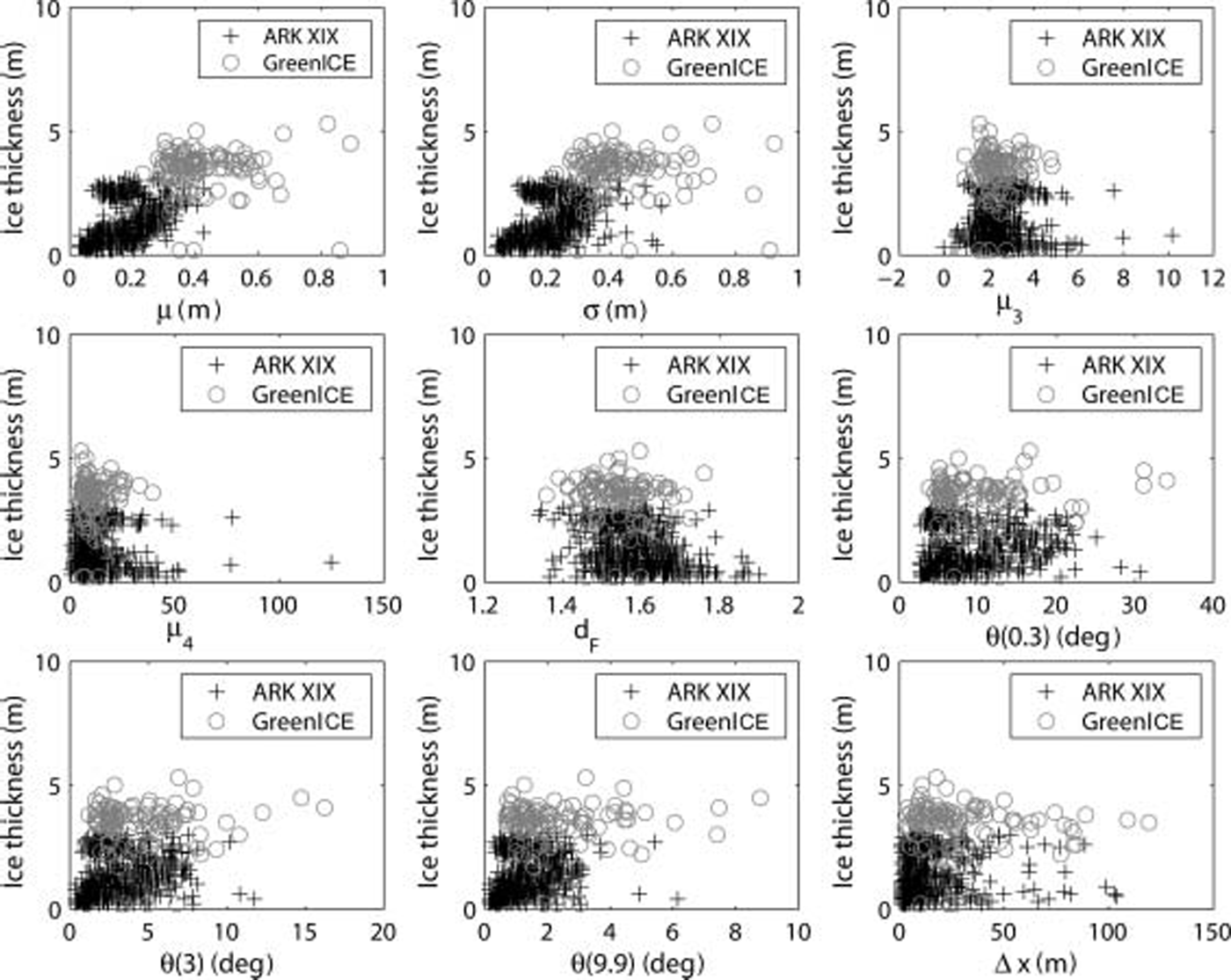
Fig. 5. Modal ice thickness vs Surface parameters for the combined dataset from ARK XIX and GreenICE (L=2km).
6.2. Fram Strait, July–August 2004
The cruise ark xx/2 took place during july–august 2004 with r/v Polarstern in the fram Strait. unlike ark xix and greenice, this campaign was carried out during the arctic Summer. as a consequence, melt ponds were present on top of the floes (estimated coverage 10–40%). melt ponds lead to an increase in Surface roughness due to the Slopes of the pond walls. this increase in roughness is counteracted by the Smoothing effect of melt processes on pressure ridges. the Surface melting thus causes complex changes in the topography.
Measurements of Surface elevation and ice thickness were obtained from laser altimetry and Simultaneous em induction Sounding as described in Section 2. after division of the profiles into 2 km long Sections, in total 149 Sections were available for classification. the distribution of the observed modal ice thickness Showed that hardly any thin ice was present, which can be attributed to the fact that it was Summer. only 15 profiles representing young, thin first-year or medium first-year ice were available, in contrast to 59 and 75 profiles of thick first-year and old ice, respectively. plots of the ice thickness vs Surface parameters reveal fairly Spherical distributions with no obvious inherent Structure. the correlation between the parameters μ and σ with ice thickness decreased for the Summer data. application of the classification rule in this case gave poor results, and it was not possible to discriminate between different thickness classes. from a Statistical point of view, the profiles from different classes had very Similar properties and could not be distinguished from each other.
7. Conclusion and Outlook
The relation between Sea-ice Surface roughness and level-ice thickness was investigated with regard to classification and discrimination of different ice regimes. here, level-ice thickness of a profile was represented by the modal thickness observed on that profile. the investigation focused on the level-ice thickness rather than the mean thickness, as it represents the typical thickness observed along a profile. Statistical parameters characterizing the roughness of ice Surfaces were extracted, and an algorithm was designed to classify the Surface profiles into different ice-thickness groups based on these parameters. five thickness classes were used, in accordance with wmo Sea-ice type nomenclature. the roughness parameters were Subjected to a k-nearest-neighbour classification algorithm in order to investigate whether different level-ice thickness is reflected in the Surface properties. different profile lengths were examined. no Strong dependence of the classification performance on the profile length was found, except for the thinnest ice class, for which the allocation error decreased from profile length 5 km to 2 km. the profile length 2 km was considered best. on the one hand, this value is Sufficiently large to derive Statistical information, while on the other hand it is Small enough to preserve homogeneity with respect to ice types within the profiles. the classification algorithm gave best results for the two thickest classes, namely thick first-year and old ice, where 67.2% and 61.6% of the profiles, respectively, were assigned correctly. these two classes could be distinguished clearly from each other and from the thinner ice classes. for young ice, thin first-year and medium first-year ice, the allocation errors were large, indicating that the Surface properties of these thickness classes were not Sufficiently different for Separating them.
In Section 6, the applicability of the classification Scheme was investigated on two different datasets. the greenice data displayed a relation of the parameters mean elevation and rms height to ice thickness Similar to that observed in the ark xix data. application of the classification to the combined datasets yielded a decrease of the within-class allocation error for old ice, due to the additional old ice profiles present in the greenice dataset, while the overall performance did not improve Significantly.
The ark xx dataset Showed that application of the classification Scheme to data obtained under Summer conditions is not feasible. even though essentially two different thickness classes were present, the roughness parameters gave no indication of the existence of different ice types. the difference in classification performance for Summer and winter illustrates that the Surface topography changes Significantly between Seasons. on the one hand, melt processes in Summer lead to a Smoothing of pressure ridges. on the other hand, the accumulation of melt ponds on top of the floes increases the Surface roughness due to the generation of vertical pond walls in former level-ice areas.
The results lead to the conclusion that the relation between modal ice thickness and Statistical Surface roughness parameters is not Sufficiently Stable to guarantee a robust classification of Surface profiles into thickness regimes. the parameters mean height and rms height were found to be indicative of the ice thickness. however, meaningful results were obtained only for the thickest ice classes. a classification into the five wmo ice types is therefore not feasible, as the modal ice thickness is not reflected Sufficiently in the Surface roughness properties of the thinner ice classes. in addition, a classification of Summer data is impossible with our method.
In the light of these results, the question arises whether the level-ice thickness is a Suitable thickness measure in the analysis presented. the Sea-ice thickness distribution is affected by thermodynamic processes, reflected in the level-ice thickness, as well as by deformation processes, which lead to rafting and ridging. the latter Strongly affect the Surface roughness in the Sense that pressure ridges appear as distinct roughness features. as the thickness of deformed ice affects the mean ice thickness, but not the level-ice thickness, future work will focus on the mean thickness.
Acknowledgements
This work was Supported by european union grants evk2-ct-2002-00146 and evk2-ct-2002-00156. we thank the participants in the field campaigns ark xix, greenice 2004 and ark xx/2 for providing laser and thickness data, and two anonymous referees for helpful comments on the manuscript.


