


1. Introduction
With limited research personnel, automated platforms for assessing conditions around vessels are likely to play an increasing part in scientific research. Many of the systems used in polar regions are not designed for autonomous use, and are used to relay images to human observers with minimal automatic processing. In this paper, we present the Polar Sea Ice Topography REconstruction System (PSITRES), a 3D camera system developed for long-term deployment aboard ice-going vessels. We detail the various deployments of this system, the public dataset of images, as well as computer vision and image processing techniques we have developed.
The crew of ice-going vessels need to maintain awareness of ice conditions around the ship, and doing so is critical for safe and efficient passage, furthermore ice conditions are important for research and archival purposes. Oftentimes, camera systems are used in conjunction with trained observers on these ships; however, these systems typically do not automate the task of extracting information about the environment. Observations are carried out by different crew members at different hours, and each person introduces their own bias. This can lead to differing results, and non-uniform sampling and reporting. Camera systems with modern computer vision algorithms are capable of extracting high-level information about the scene. The goal of developing the PSITRES was to develop an autonomous platform for observing and extracting high-level information about ice. As such, we have developed techniques for 3D reconstruction, detection, classification and image processing.
Ice observations are carried out from a variety of platforms using a standardized procedure. The Canadian Manual of Standard Procedure for Observing and Reporting Ice Conditions (MANICE) (MSC, 2005) has been widely used; more recently, shipborne ice observations have been carried out using the Arctic Shipborne Sea Ice Standardization Tool (ASSIST) (Scott Macfarlane and Grimes, Reference Scott Macfarlane and Grimes2012). Observers look at the ice 360° around the ship. Parameters such as freeboard, snow coverage, melt pond coverage, topography type and others are estimated. Some ships put a scale over the side so when the ship is moving, observers can directly measure the thickness of floes as they become upturned as the ship moves through (Worby and others, Reference Worby2008). Ice observations are done on an hourly basis, but in our experience, volunteers do not sign up for observation during the middle of the night, and if multiple observers are carrying out the observations, each can disagree or perform things differently.
We have aimed to develop the capabilities of PSITRES on a number of fronts, but it is not currently a replacement for ice observers, and will require considerable development before replacing human observers is viable. We have worked toward automating some of the measurements typically carried out by observers. These include melt pond coverage, algae coverage, 3D topography and detection of polar bear footprints. These parameters have been targeted because spring melt pond coverage is a good indicator of overall melt later in the season (Schroder and others, Reference Schroder, Flocco, Tsamados and Feltham2014), algae is an important source of primary production (Fernandez-Mendez, Reference Fernandez-Mendez2014), and polar bears present a risk to anyone working on the ice.
In the rest of this work, we will outline the camera system itself, and the algorithms we have developed, as well as the experiments we have conducted. We begin with the details of the specifications of the system, the deployments it has undergone, and the data it has collected. Following that we discuss the computer vision and image processing approaches utilized. We then discuss our experiments conducted on large volumes of image data to validate our approach. Subsequently, we detail the experimental results of our algorithms. We close with concluding remarks.
2. The polar sea ice topography reconstruction system (PSITRES)
The PSITRES is a 3D computer vision system developed for long-term deployment aboard an ice-going vessel. It was developed as a research tool for a variety of sea-ice observing tasks, with an initial focus on habitat classification.
2.1 Design and technical specifications
The PSITRES was built for long-term deployment aboard ice-going vessels. The environment in which the system operates presented many design constraints. PSITRES was first built in anticipation of the ARKXXVII/3 cruise in the summer of 2012 aboard the RV Polarstern. In order to achieve the largest possible viewing volume, we chose to mount the cameras at the highest point accessible to us, the flying bridge. To maintain stereo calibration, a rigid stainless steel frame is needed to maintain the relative orientation of the cameras throughout the entire deployment. The system is designed to mount to rails on the flying deck of a ship looking obliquely at the ice to one side of the ship as seen in Figure 1. The approximate viewing area of the camera system was determined by surveying the edges of the image on the ice.

Fig. 1. The Polar Sea Ice Topography REconstruction System, and its approximate viewing area.
The system is weatherproof, and can operate using 220 Volt European electrical systems, as well as American 110 Volt systems. The cameras mount to the flying deck rails; however, capturing and storing all the images requires a workstation computer. Gigabit Ethernet cameras were selected as this protocol supports high bandwidth at distances up to 100 m, and additionally Ethernet is available for outdoor use. This means it can tolerate harsh environmental conditions, allowing us to keep the computer storing the data inside the vessel.
PSITRES consists of two or three cameras, two acting as a stereo pair with a 2 m baseline. The stereo cameras are Point Grey Flea3 5 mega-pixel CCD cameras. These have been deployed with 8mm wide angle lenses. They are synchronized in hardware by a custom printed timing circuit. These cameras are housed in Dotworkz S-Type Ring of Fire enclosures, which are weatherproof and heated. An optional center camera is a Stardot NetCam SC, a 10 mega-pixel IP camera designed for security use. It has a wider field of view and does not need heating due to its low-temperature tolerance ( − 40°C). In practice, this camera has been used for development and providing context for images captured during development of the system. Figure 2 shows the cameras and their enclosures.

Fig. 2. The cameras used in the PSITRES. (a) One of the stereo cameras used in PSITRES. Each one has 2448 × 2048 (5 MP) resolution. (b) A stereo camera in its enclosure. Both enclosures are linked to allow for simultaneous triggering. (c) The center camera with a wider field of view and 10 MP resolution.
2.2 Deployments and data
PSITRES has been successfully deployed on three separate research expeditions in ice-covered waters. These expeditions were completed aboard three separate vessels in different parts of the Arctic and at different times of the year. It has imaged various ice types ranging from thin newly forming ice, to first-year floes, to multiyear ice.
In 2012, PSITRES was first deployed aboard the RV Polarstern for 80 d over a large region of the central Arctic, as well as the Berentz, Kara and Laptev seas. This expedition, the ARKXXVII/3 cruise, was the longest and northernmost for this system, covering more than 8750 nautical miles, and reaching as far as 89.283° North. For PSITRES's first deployment, the stereo cameras were triggered at a rate of 1/3 frames per second (FPS), and the center camera was triggered at 1 FPS. PSITRES operated for over 39 d, the vast majority of the time spent in ice-covered waters. In total, PSITRES recorded 2 700 285 images totaling 1.17 TB.
In 2013, PSITRES was again deployed, this time aboard the Oden, a Swedish icebreaker as part of the Oden Arctic Technology Research Cruise (OATRC 2013). OATRC brought PSITRES to the Fram Strait and the Greenland Sea with larger multiyear floes due to the transpolar current (Thomas and SDieckmann, Reference Thomas and SDieckmann2009). For this deployment, the frame rate of the stereo cameras was increased to ~2 FPS as the shorter cruise and larger hard drive capacity allowed for higher temporal resolution. The central camera remained at 1 FPS. This allowed PSITRES to capture 3 006 554 images totaling 1.46 TB.
For its most recent deployment, PSITRES was installed and operated aboard the RV Sikuliaq, an American ice-capable research vessel for its maiden expedition in ice-covered waters, the SKQ201505S cruise. This cruise through the Bering Sea began on 19 March 2015 and lasted 25 days. For this cruise, the stereo cameras were triggered at ~2 FPS; however, the central camera was not deployed to save time. PSITRES captured 2 341 876 images totaling 1.87 TB.
In total, PSITRES has spent 118 d at sea, collected 8 048 715 images or 4.5 TB of data, endured snow, ice, gale force winds, and has suffered only one unexpected shutdown. The system is reliableand capable of running for days on end with little intervention. It has proven robust in diverse environments of the geographic locations. The diversity of the platforms on which it has been deployed testify to its readily deployable nature. The system, once installed and calibrated, needs only basic maintenance in the form of ice removal when necessary.
The image data captured by the PSITRES camera system are truly unique. No other stereo camera system has been deployed in such an environment, offering certain capabilities unmatched by 2D counterparts. However, the data itself present numerous challenges to typical computer vision techniques. There are complications due to rain, fog and snow, and many other environmental issues. In spite of these difficulties, one of the largest problems is the sheer volume of data. With over 8 million images, many traditional image processing approaches become completely unfeasible. For example, a process taking just 1 min per image would require more than 15 years to complete if run sequentially. To combat these problems, we have developed new algorithms and have subsampled the dataset for different tasks.
The raw image data, as well as derived data products, are available at https://vims.cis.udel.edu/geo/ice/. This site will be updated with new elements as we develop new approaches and acquire new data. Additionally, we will be providing metadata in the form of data provided by other onboard sensors, such as GPS, and heading.
2.3 Comparison to other camera systems
PSITRES is not the first camera system to be deployed aboard ice-going vessels, and while its capabilities and specific goals are unique, many other systems have been deployed with the overall goal of extracting information about the environment around the ship. In this section, we will briefly discuss several camera systems and compare them to the PSITRES.
Eiscam 1 and 2 are monocular camera systems developed by Weissling and others (Reference Weissling, Ackley, Wagner and Xie2009) to observe a swath of ice and water adjacent to an ice breaker. Both Eiscam were deployed aboard the icebreaker NB Palmer, during the 2007 SIMBA (Sea Ice Mass Balance in Antarctic) cruise. The systems recorded at 3 and 10 frames per minute, respectively, recording at 480 television lines (TVL), in an analog picture format typically with a digital resolution equivalent of 510 × 492. In order to obtain quantitative measurements of the ice, the images were orthorectified by manually surveying the viewing area of the cameras. The system was used to derive ice concentration, ice types, floe sizeand area of deformed ice. These 2D parameters require careful selection of image sequences however, as ship roll is unaccounted for. Both cameras operated for ~125 h over the course of ~900 km of transit.
In 2009 and 2010, a group from Tokai University Research and Information Center in Japan constructed and tested a stereo camera system aboard a small icebreaker in the Okhotsk sea in the north of Japan (Niioka and CHO, Reference Niioka and CHO2010). The system was mounted aboard the sightseeing icebreaker the Garinko-2, in the Monbetsu Bay of Hokkaido. The system was mounted 2.5 m above sea level with a viewing area of a few square meters. The system was not built for full 3D reconstruction of ice, but was used to manually measure the cross-sectional thickness of upturned floes. The system recorded data over a few kilometers, taking ~30 image pairs that were evaluated manually.
Unlike these other systems, PSITRES was purpose built for high-resolution reconstruction of ice. It features a small pixel footprint, and can be used to measure 3D objects in real-world units. The camera system developed by Tokai University Research and Information Center is the only other 3D system, and therefore most readily compares to PSITRES. However, they have been developed for different tasks. PSITRES's viewing area is larger than this system, and it has been developed for fully automatic reconstruction with minimal human involvement. Furthermore, PSITRES has been developed to capture large volumes over long-term deployments in remote regions.
3. Computer vision methods
In this section, we will detail different computer vision and image processing algorithms developed for data collected by the PSITRES camera system. These include methods for stereo reconstruction, segmentation and detection of polar bear footprints, as well as algae and melt pond detection. While we have attempted to write this section so that it is clear to a wide audience, many of the algorithms discussed are ongoing research topics in the field of computer vision. We direct the reader to ‘Multiple View Geometry’ by Hartley and Zisserman (Reference Hartley and Zisserman2003) for an overview of many 3D reconstruction and computer vision approaches.
3.1 3D scene reconstruction
Stereo vision is a technique of using two images to generate a 3D model. This technique is a form of bio-mimicry that emulates one of the ways eyes perceive depth. Coarsely speaking, the scene forms two images on the different cameras, and then points in these images are matched and 3D position can be triangulated.
To begin discussing 3D computer vision, it is important to start with the camera model, and how projection of points in a 3D scene onto an image is modeled. The pinhole camera is used for many tasks in computer vision. Intuitively, this is a point in 3D space with a vector defining the direction the camera is looking. To simplify matters, we treat the left camera of the stereo pair as the origin of our coordinate system, and its look vector along the positive Z dimension. Mathematically, the camera can be modeled by the 3 × 3 matrix $\left[\matrix{ f_x & s & x_0 \cr 0 & f_y & y_0 \cr 0 & 0 & 1 }\right]$ where f x and f y are the focal lengths in the X and Y dimensions of the image, and s models image skew. (x 0, y 0) is the coordinates of the ‘principal point’ or the intersection of the camera's view vector with the image plane, in image coordinates.
Projecting a point from the 3D scene to the corresponding image point is simply a matter of multiplying this camera matrix and the 3D vector of the point's location. The X and Y terms resulting 3D vector are then divided by the Z component resulting in the image coordinates of the 3D point.
To project points to the right camera which is not centered at the origin, we apply the inverse of the transformation of the camera to the points, and project them using the same scheme. In order to identify these parameters, calibration is needed.
Stereo calibration is the process of fitting a model to the physical properties of the camera setup. This model incorporates the intrinsic parameters of the cameras, encapsulating lens parameters, the extrinsic parameters which model the translation and rotation of the different cameras. The process of calibrating PSITRES involves photographing a calibration pattern (a planar checkerboard) and using an optimization framework to iteratively improve estimates for the various parameters based on Zhang (Reference Zhang2000). This involves using the 3D position of the corners of each square on the checkerboard to solve for the intrinsic and extrinsic parameters of the camera system and the position of the system relative to the calibration board by over-constraining a system of equations. PSITRES was calibrated at ice stations by bringing a large checkerboard pattern onto the ice and into its viewing area, as shown in Figure 3. Once calibrated, matching pixels can be triangulated by identifying the closest point of intersection of two rays going from the camera pinhole through the image plane into the 3D scene.

Fig. 3. Calibrating the system at an ice station using a checkerboard calibration pattern.

Fig. 4. A sample point cloud reconstructed from PSITRES imagery, showing a small ridge.
3.1.1 Reconstruction
After calibration, stereo image pairs can be reconstructed by matching points in each image and finding the closest intersection of rays created by corresponding pixels. To do this, the images are first rectified as the cameras on PSITRES are not co-planar. The relationship between a given image point and its matching point on the other image is called epipolar geometry. Epipolar geometry relates corresponding points between images according to the depth of the scene point. Rectifying the images allows us to transform the images such that correspondences lie on horizontal scanlines. Rectification is done using uncalibrated techniques (Forsyth and Ponce, Reference Forsyth and Ponce2003). This allows for dense matching using disparity estimation.
Disparity estimation, or disparity matching, allows for dense correspondences between two stereo images. The resulting correspondences are often called a disparity map. Computing the disparity map of a given set of images is however not trivial and there are numerous techniques that have been developed in this line of research. In image regions where there is little texture information, the problem is inherently ill defined (Baker and others, Reference Baker, Sim and Kanade2001). This poses a problem for scenes with large areas with little image texture information such as those with uniform ice. We have used low texture matching techniques (Rohith and others, Reference Rohith, Somanath, Kambhamettu and Geiger2009) to generate dense correspondences between stereo pairs, and these correspondences are triangulated according to the calibration parameters to yield dense point clouds in metric scale (using real-world units).
After reconstructing a 3D scene, we are left with a 3D point cloud (set of 3D vertices with associated color values) in real-world units, which allows us to quantify the physical properties of the sea-ice surface. First, we fit a plane to the 3D point cloud using Principle Component Analysis (PCA). The coefficients from PCA give a surface normal for a plane that best fits to the 3D point cloud. We then compute a centroid and take it to define a plane using point-normal form.

where P is a point in the plane (the centroid), n is the plane normal and d is a constant. We solve for d, and this allows us to define the plane implicitly as

where a, b, c are the coefficients from PCA.
This plane allows us to measure 2D image regions in real-world units via reprojection. Projecting 2D components while preserving scale can be done by calculating the homography between the image plane and the scene plane. This requires four correspondences (Goshtasby, Reference Goshtasby1986, Reference Goshtasby1988). Since both planes are defined in the same coordinate system, we generate correspondences by randomly selecting points in the scene plane and projecting them to the image plane. To convert to homogeneous coordinates, the scene plane is defined in terms of a point on the plane, P, and two linearly independent vectors contained within the plane, $\overrightarrow {b_1}$ and $\overrightarrow {b_2}$
 .
.
In this implementation, P is the centroid of the point cloud, and $\overrightarrow {b_1}$ and $\overrightarrow {b_2}$
 are the first and second coefficients obtained from PCA of the point cloud. Using randomly generated numbers Q and R, we generate points on the plane using

The homogenous coordinate is then (Q, R). The corresponding point on the image plane, $\overrightarrow {x_{2i}}$ , is the projection of $\overrightarrow {x_{1i}}$
 onto the image using the camera parameters obtained from calibration. S is a scale factor relating pixels to the units of the 3D model, and is used to determine the size of the resulting reprojection. This allows us to reproject the image and maintain scale similar to the orthorectification technique used in Weissling and others (Reference Weissling, Ackley, Wagner and Xie2009).
The surface roughness of sea ice is an important geophysical parameter that effects momentum transfer from the atmosphere to ice (Cole and others, Reference Cole2017) and the suitability of the ice pack as habitat for marine mammals (Ferguson and others, Reference Ferguson, Taylor and Messier2000). Surface roughness is affected by dynamic processes such as ridge-building as well as summertime melt processes in the case of multiyear sea ice. Following the approach described by Manninen (Reference Manninen1997), we can parameterize ice surface roughness using the root-mean-square (RMS) distance of all the vertices in the point cloud, P x, from the fitted plane:

where D i is point-plane distance. Surface roughness is then measured using RMS point-plane distance from the fit plane by

3.2 2D sea-ice parameters
We have developed a novel technique to rapidly detect algae and melt ponds present in PSITRES images using a color space transformation and vectorized thresholding scheme. This technique was developed for real-time detection and the emphasis is on computational efficiency. We have modeled these parameters in terms of their surface extent, and therefore only 2D measurement is needed.
3.2.1 Color space transformation
We have utilized a novel color transformation and thresholding scheme which is fast and discriminative. The transformation is expressed as $f\lpar rgb\rpar = {\opf N}_3 \rightarrow {\opf N}_4$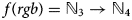 and transforms pixels from RGB to RGBI or red, green, blue, intensity space. It is computed:

This formulation is independent per pixel and is easily parallelized. Moreover, it is incredibly fast, requiring on average 0.0258 s per image. On its own, m is similar to a grayscale image but with darker artifacts. At least one of r − m, g − m, b − m will be 0 for a given pixel. This transformation preserves the relative differences between channels, making it robust to slight differences in illumination or intensity. The RGBI color space is also discriminative of colored regions in scenes where the primary variation is in luminosity, such as PSITRES images. These properties make it well suited for segmenting out melt ponds and algae, each of which can be distinguished from the ice.
3.2.2 Segmentation scheme
Segmentation is carried out on a per channel basis and is formulated formally for every pixel p i = {R i, G i, B i,} where R i, G i and B i are the red, green and blue color channels, we compute

We use two vectors,

and

where t r, t g, t b, t m, are the thresholds along each channel, and u = u r, u g, u b, u m is a four-element trinary vector with three possible values, indicating whether the threshold should be done using the ≤ or ≥ operator or the channel should be ignored. The individual results are combined together using logical AND. Like many threshold-based methods, this can lead to noisy segments. To mitigate this, morphological closing and opening are used. We use a small diamond-shaped structuring element of a radius of 12, as this is an efficient process which deals with most of the noise in these images.
PSITRES records an area adjacent to the ship, and as a result, the animals who are wary of a large, noisy ship do not often enter the field of view of the cameras. During the ARKXXVII/3 cruise, in 2012, PSITRES observed a large number of polar bear footprints, and we have developed a technique for detecting these prints in PSITRES images using a Convolutional Neural Network (CNN) (Sorensen and others, Reference Sorensen2017). We have trained a CNN to classify image patches as containing prints or not.
We have created a training and testing dataset by manually labeling ~5000 prints in PSITRES images. We extract a small patch around each print, and experiment with different patch sizes. We have collected an identical number of patches that do not contain prints from elsewhere in the same scenes to create a set of negative samples. Figure 6 shows a few positive samples with prints and negative samples for a patch size of 160 × 160.
Training is done using a transfer learning for classification. We treat the problem as a binary classification of patches containing polar bear prints or patches without polar bear prints. We initialize the network using the InceptionNet (Szegedy and others, Reference Szegedy2014) implementation in Google's Tensor Flow deep learning framework (Abadi and others, Reference Abadi2015). The network architecture is shown in Figure 5.

Fig. 5. InceptionNet architecture (Szegedy and others, Reference Szegedy2014).

Fig. 6. Positive samples with patches (left three images), and negative samples without patches (right three images).
The network was originally trained on the ImageNet Large Scale Visual Recognition Challenge dataset (Russakovsky and others, Reference Russakovsky2015) which consists of 1000 different image classes. This network consists of 22 layers, composed of convolution, pooling and softmax operations. This architecture was designed so that they are not fully connected to the previous layer, followed by aggregation in the form of pooling. This allows the network to perform well without drastically increasing the size. We have formulated our problem as a binary classification. To accommodate the large change in the number of labels, we have modified the network using a new softmax layer with the corresponding number of outputs to the classification domain (positive samples containing prints and negative samples containing no prints).
4. Experiments and results
We have conducted a number of experiments to assess the validity of these approaches as well as assess their viability toward processing large volumes of images in reasonable time frames.
4.1 Color space transformation and segmentation
In this section, we compare the colorspace transformation and segmentation technique described above and discuss performance both in terms of accuracy and speed. Tests have been conducted on the same machine, with a Core i7-4930 k CPU and 64 GB of RAM. For results specified as using Matlab, Matlab 2014A was used and C++ results using OpenCV 3.4.9 and gcc 4.6.3.
To test the segmentation approach, two experiments were conducted. First we focused on timing, as accuracy depends on the threshold selected, however computation time does not. We compare with fourtraditional color transformations. Each approach was tested on a set of 50 images and the mean is reported. Timing results are shown in Table 1. It is clear that this transformation is well suited for big data. Application of the threshold is quite fast, taking 0.0376 s, and the morphological operations take 0.126 s. In total, this scheme takes 0.174 s, meaning the entire dataset could be processed in a little less than 12 d.
Table 1. Color space transformation times

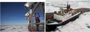
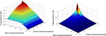
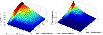
To evaluate the accuracy, we have manually labeled 50 images containing algae and melt ponds and iterate over each possible value on two channels (melt ponds along green and blue channels and algae along red and green). Results are shown in Figures 7 and 8. This scheme performs well for classifying melt ponds, but algae is a more difficult task as it appears as a subtle difference in color in small regions. Furthermore, even under ideal performance, this sort of technique would only work for algae that is visible at the surface, so is unlikely to be useful for measuring biomass, for example. Figure 9 shows some results of the proposed segmentation scheme.

Fig. 7. True- and false-positive rate for melt ponds.

Fig. 8. True- and false-positive rate for algae.

Fig. 9. Segmentation using the proposed scheme. The top row shows the input image with results on the bottom row for melt ponds (bright region, left), algae (bright region, center) and open water (red region, right).
4.2 Paw print detection
To test our convolutional neural network classifier, we have used ten-fold cross-validation. This means we train ten models with non-overlapping testing sets spanning our data. We evaluate accuracy on the testing set for each fold and average the results. The main criterion for evaluation is accuracy on the testing set averaged across each fold. In the following subsection, we discuss different patch sizes used.
4.2.1 Patch size
Since we extract patches around individual prints (which can contain other prints), we have experimented with different patch sizes to evaluate how this affects accuracy. We measured cross-fold validation accuracy on eight different paw print datasets of varying size. These patches range from 20 × 20 pixels to 160 × 160. Figure 10 shows the accuracy at different scales and includes the average across all ten folds as well as the performing classifier at each scale. We found a larger patch size resulted in higher accuracy, so our resulting accuracy of 90.67% corresponds to a patch size of 160 × 160.

Fig. 10. Detection accuracy for different patch sizes.
Below we will discuss the results of applying these algorithms to large portions of the PSITRES image data. In practice, these experiments are done to subsets, typically one cruise at a time, as these techniques can require considerable processing time.
4.3 3D results
We have used the low texture stereo technique and carried out a large-scale experiment in reconstructing pairs from the OATRC 2013 cruise aboard the Oden. We have reconstructed every 50th synchronized pair of images (which corresponds to roughly every 20 s) and evaluated the surface roughness of each scene. The resulting roughness estimates are noisy, so we have applied a 1D running Gaussian filter over 100 samples. The results are shown in Figure 11. These results show variance in a physically plausible range. They are however likely an overestimate, as ships would avoid larger ridges.

Fig. 11. Surface roughness measured during the OATRC 2013 cruise.
4.4 Algae and melt ponds
We have used the techniques described above to identify algae presence as well as melt pond fraction throughout the cruise track of the RV Polarstern during the ARKXXVII/3 cruise. To do this, we have used just the left stereo images, as the right image would be almost identical and is therefore redundant. We compute the fraction of coverage in terms of fraction of the image. Admittedly, this is not a true measurement for something like melt pond fraction, but in the process of manual ice observation, these parameters are reported per floe type, and we have not addressed many of these broader issues in developing a proof of concept. We present the results in the form of North Polar Stereographic maps of the cruise track with color representing concentration. For each map, concentration is the portion of pixels classified as containing algae or melt ponds naively ignoring spatial pixel coverage. The results for melt ponds are shown on the left in Figure 12 and algae results are shown on the right.

Fig. 12. North Polar Stereographic Map of detected melt ponds (A) and algae (B) for the ARKXXVII/3 cruise.
4.5 Polar bear prints
We have used the best trained CNN to identify prints across the entire cruise track. We have subsampled PSITRES images at a rate of approximately one image every 5 min. Each image was split into equally sized patches and the patches were classified using the trained model. The resulting frequency of patches was then filtered using a moving average filter over ten samples. Results are shown in Figure 13. Vertical lines denote days with photographed sightings of bears, and days with ice stations where humans would appear on the ice.

Fig. 13. Polar bear paw print frequency over the entire ARKXVII/3 cruise. Red vertical lines indicate days for which we have photo evidence of bears, and green lines indicate days with ice stations, where there are likely to be human prints.
These results show peaks on days where polar bears were spotted, including a strong peak on 17 September where over a dozen bears were sighted, but also shows peaks at days with ice stations, such as around 14 August, where many of these tracks were left by humans. The classifier was not presented with the challenge of classifying bear prints and human prints separately, and as a result identifies human prints as well.
4.6 Comparison to ASSIST observations
We have compared these results with ice observations made during the cruise to facilitate a comparison with available data. ASSIST (Scott Macfarlane and Grimes, Reference Scott Macfarlane and Grimes2012) reports ice parameters in terms of partial coverages based on different ice types. This means that algae, melt pond and 3D parameters are reported per ice type, and up to three can be reported during a single observation. Since PSITRES reports these values over an entire scene, we have aggregated ASSIST results. For melt ponds, total coverage T MPC is calculated using

where e is either primary, secondary or tertiary, PC is the partial coverage, and MPC is the melt pond coverage.
Using ASSIST, algae is reported more coarsely aggregated into the categories of 0, < 30, < 60 and $\gt 60\percnt$ . We have collapsed these ranges into discrete values to facilitate aggregation. These values were selected for partial coverage eA as eA = {0, 0.25, 0.5, 0.75}. Scene level algae coverage, T A, is then calculated using

For 3D comparison, we have used ridge height as a 3D measurement for which to compare. Surface roughness is not directly reported in the ASSIST framework; however, large ridges would contribute heavily to surface roughness changes over level ice, and so we expect these values to correlate. ASSIST reports ridge height in terms of ice types as well so we calculate the weighted sum ridge height T RH by

We have averaged PSITRES results over corresponding 1 h periods and compared these results in the graphs below. We have also carried out statistical analysis in the form of measuring the Pearson Correlation Coefficient of the two sequences and the results are reported in Table 2. Figure 14 shows resulting algae estimate comparison. Figure 15 shows a comparison for melt ponds. In the case of comparing algae concentration, there are some confounding factors that likely affect reported observations. Some observers did not report algae concentration, which is shown in the fluctuating reports. Additionally, days later in September had significantly less light and more oblique lighting.
Table 2. PSITRES ASSIST correlation


Fig. 14. Algae as estimated by the PSITRES and ASSIST observations.

Fig. 15. Melt pond coverage as estimated by the PSITRES and ASSIST observations.
5. Conclusion and discussion
Results presented in this paper show that an automated camera system can be used to supplement the role of trained ice observers. In polar summers, constant daylight allows for round-the-clock operation and an automated platform does not exhibit the same biases and potential for errors that humans do. This is not to say that the camera system is perfect, and we are actively developing both the hardware and software. These results are a starting point, and as we develop new techniques, we will improve upon them. We will make our data and the results of our continually developed algorithms available to the community.
In the future, we hope to continue to develop the capabilities of the PSITRES camera system. We are developing real-time techniques for the camera system to allow it to be reliably used during a cruise, as opposed to processing the data after the trip. We are exploring more deep learning approaches to develop robust techniques for estimating other key parameters of sea ice, and to leverage GPU hardware for real-time processing while underway.
We intend to improve the physical robustness and ease of deployment by creating a self-contained system that can be more easily mounted and deployed by someone unfamiliar with the system. On the software side, improvements to robustness and ease of use are also a priority. Requiring an expert user for assembly, calibration and maintenance limits the scope of deploying PSITRES and it is our goal to eliminate these barriers.
In this work, we have presented the PSITRES, a 3D camera system capable of high-resolution 3D reconstruction, and algorithms for automated extraction of parameters related to sea ice. PSITRES has been successfully deployed on three separate research expeditions in Arctic and Subarctic. We have also presented a series of computer vision and image processing techniques we have developed to extract high-level information about conditions around the ship. These techniques are aimed at extracting some of the more important parameters of sea ice, and ones that are reported by trained ice observers.


 Open access