

Introduction
The contribution to sea-level rise of Arctic glaciers, excluding the Greenland ice sheet, under climate-change scenarios is likely to be significant. For example, Reference DowdeswellDowdeswell and others (1997) estimated that Arctic glaciers, excluding Greenland, contribute about 5% of the current observed sea-level rise (or 0.13 mma–1). The Arctic mountain glaciers and island ice caps display a spatial and structural diversity. Circum-Arctic glaciers can be found in climatic zones ranging from dry high-Arctic climates to maritime Norway, and thus their current mass balance differs widely. White Glacier, Canadian High Arctic, had a net balance of –4.01 and –1.81mw.e. in 2000 and 2001 respectively, whilst Engabreen, Norway, had a net balance of +14.90 and –15.30 mw.e. in those years (Reference Haeberli, Frauenfelder, Hoelzle and ZempHaeberli and others, 2003). Therefore a distributed observation programme is required for monitoring the response of circum-Arctic glaciers to climate change. Monitoring data would provide a valuable insight into the spatial variation in glacier–climate interactions and the dynamic response of different glacier types to climatic forcing.
Amplitude SAR data have been used to map glacier features such as end-of-summer snowline (Reference Brown, Kirkbride and VaughanBrown and others, 1999), winter firn edge (Reference Hall, Williams, Barton, Smith and GarvinHall and others, 2000) and backscatter zonation (Reference PartingtonPartington, 1998; Reference König, Wadham, Winther, Kohler and NuttallKönig and others, 2002). In the dry-snow zone of Greenland, backscatter has been inversely correlated with snow accumulation (Reference Forster, Jezek, Bolzan, Baumgartner and GogineniForster and others, 1999). Reference Engeset, Kohler, Melvold and LundénEngeset and others (2002) attempted to relate specific net balance and backscatter on Kongsvegen, Svalbard, but found only proxy data could be extracted. There has been no definitive relationship between specific net balance or winter balance measurements and SAR backscatter from temperate glaciers.
In this paper, we analyze the processes affecting synthetic aperture radar (SAR) backscatter from two Arctic glaciers. We have acquired RADARSAT-1 SAR imagery over Blåmannsisen, an ice cap in north Norway, and Salajekna, a valley glacier on the Swedish–Norwegian border (Fig. 1). The paper examines the composition of SAR backscatter using coupled surface and volume backscatter models, and compares it to observations made using RADARSAT-1 standard beam imagery. Field data are used to constrain the models, and the effect of changing specific winter balance is modelled. From these results we show that terms such as surface roughness can be more important to SAR backscatter on these glaciers than differences in net accumulation between years. These results support similar observations by Reference De Ruyter de Wildt and Oerlemansde Ruyter de Wildt and Oerlemans (2003) on another temperate glacier, Vatnajökull, Iceland.
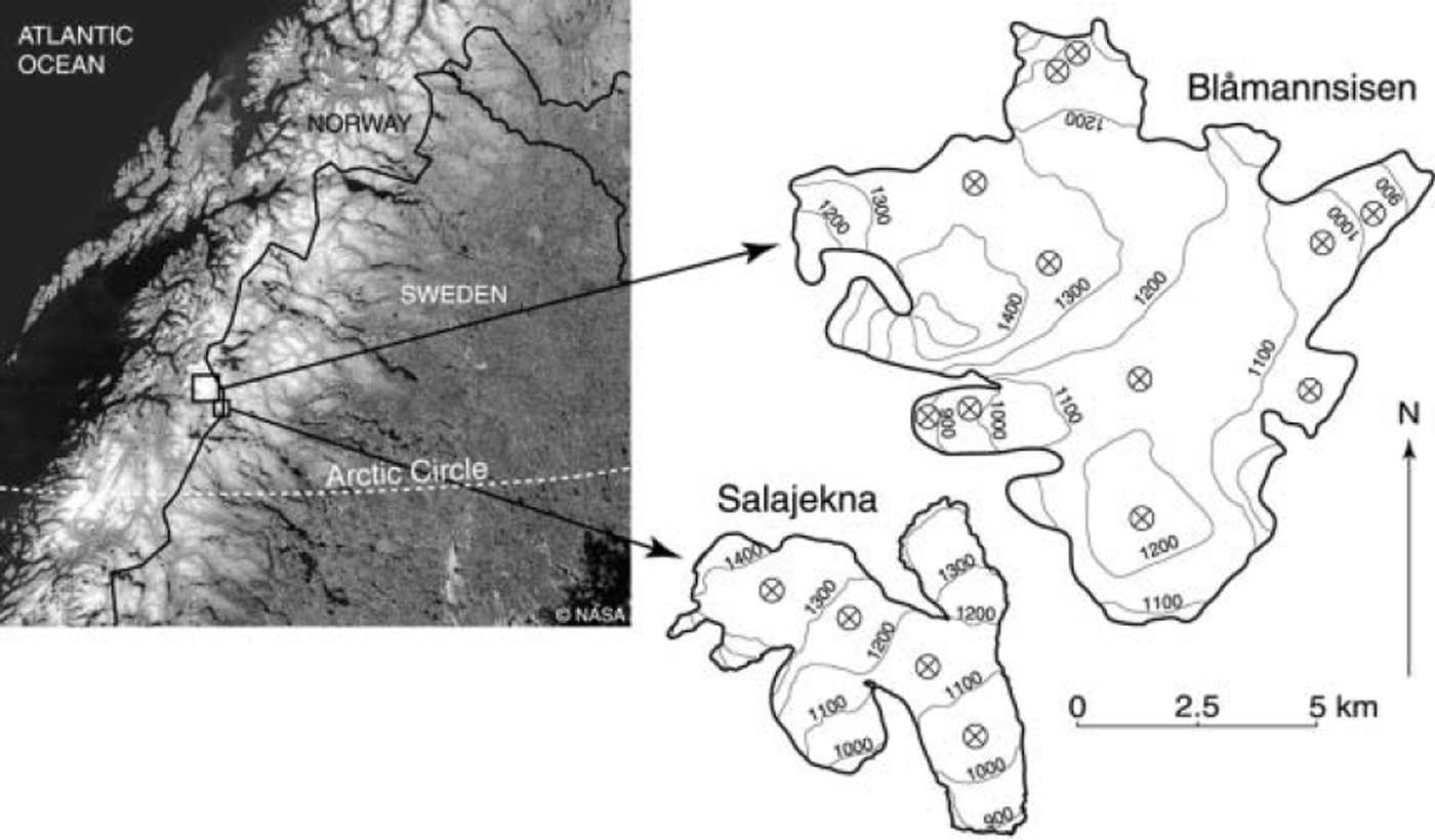
Fig. 1. A location map showing Blåmannsisen and Salajekna. Both glaciers are temperate and lack dry-snow facies. The ⊗ symbols indicate the location of sampling points in the SAR imagery.
Backscatter Processes and Modelling
Radar waves interacting with a target are scattered at the interface with the air (surface scattering) and from within the target (volume scattering); there may be a further contribution to the total backscatter from subsurface layers. Surface scattering is primarily dependent on the surface roughness, permittivity (dielectric constant) and the imaging geometry. Volume scattering results from dielectric discontinuities within inhomogeneous media such as snowpacks (Reference Curlander and McDonoughCurlander and McDonough, 1992; Reference FungFung, 1994). Backscatter at centimetre wavelengths, such as from a glacier in winter, typically comprises surface scattering from the air– snow interface, and from the snow–ice interface in the bare-ice zone; volume scattering occurs in the snowpack and in the firn (Reference PartingtonPartington, 1998; Reference Forster, Jezek, Bolzan, Baumgartner and GogineniForster and others, 1999). The presence of liquid water reduces transmissivity, increases absorption and causes a reduction in the penetration depth of the radar waves. In the presence of liquid water, surface scattering may be enhanced but volume scattering is significantly reduced. In some cases, the increase in the dielectric contrast at the air–snow interface may paradoxically increase backscatter by offsetting the loss of volume scattering against larger surface scattering.
Semi-empirical scattering models are useful tools for examining the composition of backscatter. Such models can be used to decompose backscatter into its various components (surface, volume and secondary surface scattering). Alternatively, backscatter models can be used to identify the likely response of backscatter to environmental changes. Surface scattering models typically parameterize the roughness of the surface relative to the radar wavelength, the imaging geometry and permittivity (Reference Barber and LeDrewBarber and LeDrew, 1994; Reference FungFung 1994). The complexity of such models is in part represented by the parameterization of the surface roughness. Solutions are normally based on either a Gaussian correlation function in simpler models or a Fourier transform in the more complex models. Here we use a simple geometric optics formulation of a Kirchhoff scattering model to estimate backscatter from a rough snow surface (Reference Barber and LeDrewBarber and LeDrew, 1994; Reference GuneriussenGuneriussen, 1997), and the small-perturbation model (SPM) for smoother surfaces (Reference FungFung, 1994; Reference ReesRees, 2001).
The Kirchhoff model is given by:
where denotes parallel polarization, 9 is the incidence angle, ||(0) is the Fresnel reflection coefficient for normally incident radiation at nadir and m is the root-mean-square (rms) surface slope which is given by:
where l is the correlation length and Δh the rms height variation. The rms height variation is the simplest measure of the roughness of the surface above a reference plane. The correlation length is a measure of the width of these irregularities (Reference ReesRees, 2001).
Smoother surfaces can be modelled using the SPM:
where σ°||(θ) denotes the backscatter from a co-polarized wave at a given incidence angle, f||(θ) is a measure of the reflectivity for co-polarized radiation defined as
k is the wavenumber and ε2 the complex dielectric constant of snow.
Volume scattering is represented in scattering models by the dielectric properties of the medium and its morphometry (commonly represented by the grain-size and number density). Here we use a Rayleigh approximation to model the volume scattering from a snowpack (Reference GuneriussenGuneriussen, 1997; Reference Forster, Jezek, Bolzan, Baumgartner and GogineniForster and others, 1999; Reference Nagler and RottNagler and Rott, 2000):
where σ°b is the average scattering cross-section from a snow grain, κe is the extinction coefficient, L is the one-way propagation loss and N is the number density of the scatterers, which is calculated from:
where v is the volume fraction of snow and r is the grain radius. The value of σ°b is calculated according to:
where λ is the wavelength of the SAR and K is a term describing the dielectric properties of the scatterers in relation to the background medium.
The volume-scattering model employs a correction for near-field effects in dense media (Reference Shi, Davis and DozierShi and others, 1993; Reference Forster, Jezek, Bolzan, Baumgartner and GogineniForster and others, 1999):
This correction introduces an optically equivalent grain-size which is usually larger than the physical grain-size in snow but smaller than the grain-size in firn. The integration of the models is weighted by the transmissivity of the medium and the propagation loss to account for extinction within the volume (Reference Barber and LeDrewBarber and LeDrew, 1994; Reference GuneriussenGuneriussen, 1997). Surface scattering between snow and firn layers is ignored (Reference Forster, Jezek, Bolzan, Baumgartner and GogineniForster and others, 1999). Where not measured in situ, the permittivity and dielectric loss were calculated according to Reference FungFung (1994, appendix 9A). The imaginary part of the complex dielectic constant for glacier ice was estimated from Reference Matsuoka, Fujita and MaeMatsuoka and others (1996), because measurements were not possible.
SAR Data
The integrated model is used to improve our analysis of the processes affecting backscatter in RADARSAT SAR imagery. Our image dataset includes RADARSAT standard beam modes 1-3 scenes acquired between 2000 and 2002 (Table 1). The images were processed using the Alaska Satellite Facility’s STEP software. Samples of 625 pixels, extracted from a 25 × 25 pixel window, were corrected for topographic effects using three-dimensional angles derived from photogrammetric digital elevation data with a 25 m grid size. A topographic correction, a, derived from weighting the inverse sine correction (Reference Laur, Meadows, Sanchez and DwyerLaur and others, 1993) with the spherical geometry solution of Reference UlanderUlander (1996), was used after adjusting for slant-range to ground-range effects (Reference UlanderUlander, 1996):
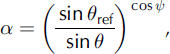
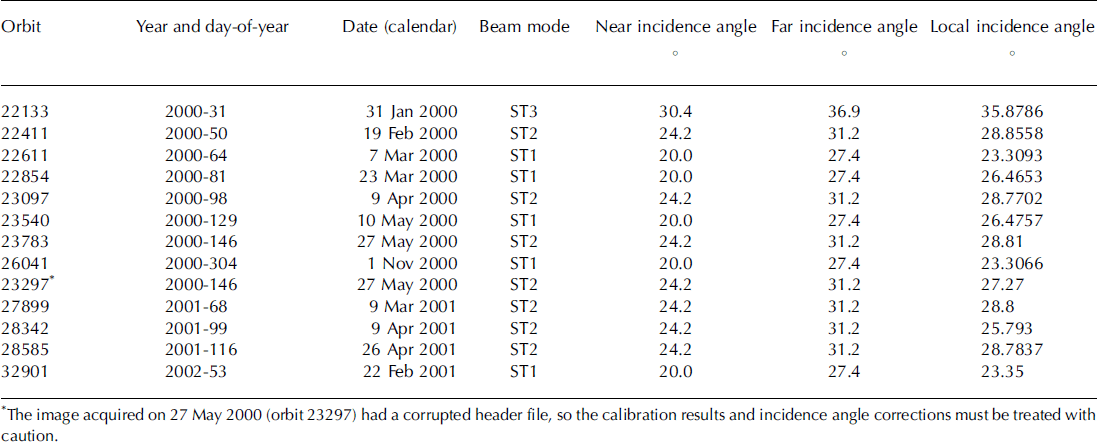
Table 1. The SAR image properties for the images used in this study
where θ re f is the reference incidence angle (23°) and is the angle between surface normal and image plane normal.
This solution introduces a correction for surface tilt in range and azimuth rather than the simple range solution often used (Reference Laur, Meadows, Sanchez and DwyerLaur and others, 1993; Reference GuneriussenGuneriussen, 1997). The effect of varying satellite altitude on the calculation of local incidence angle was estimated, but the incidence angle difference was lower than the confidence in the elevation data, so a constant (average) satellite altitude was used (802.4 km).
Field Measurements
Field observations are required in order to constrain the model. Measurements of dielectric constant, liquid-water content and winter, summer and net balance were made intermittently between 1998 and 2004 on Salajekna (Reference KlingbjerKlingbjer, 2004). Similar measurements, excepting the surface net, winter and summer balance, were made on Blåmannsisen. Snow pits 1.5–3 m deep were excavated. Snow density was calculated using samples collected in a cylinder of known volume; dielectric constant was measured with a Denoth-type flat capacitance probe; and snow depth was also measured by probing. Typically snow-pit measurements were made every 20cm (each measurement being 8cm in diameter). Firn cores were also acquired in 2002 and 2004 from Blåmannsisen to constrain the modelling of the upper firn (3–8 m deep). Ground-penetrating radar (GPR) was used to measure the firn–ice transition depth on Blåmannsisen to allow us to extrapolate the firn measurements. Frequencies between 800 and 3000MHz were used to observe the firn–ice transition which normally occurs at depths of 12–15 m. The extrapolation from the measured density used the observed depth–density curve extrapolated to 12m. This increased backscatter by 1 dB compared with the 8 m measurement, emphasizing the role of near-field effects in dense media. Field measurements were made approximately contemporaneously with satellite overpasses on three occasions (10 May 2000, 27 May 2000 and 24 April 2001).
Results
Field results
The mass-balance data show that Salajekna is approaching equilibrium (Reference KlingbjerKlingbjer, 2004; Fig. 2). Although few data exist, the winter and net balance appear strongly correlated, suggesting the winter component of the net balance may have a stronger influence than summer balance. In mass-balance year 2000 the specific net balance was +0.10 mw.e. with a specific winter balance of 2.30 mw.e. Salajekna had a very negative balance (–0.8m w.e.) with a specific winter balance of 1.31 mw.e. the following year. The SAR image from early 2002 suggests that firn thinning may have occurred near the firn limit during the previous summer. GPR data from 1998 showed firn thinning as a result of melting at the surface had occurred at some time in the recent past. An Advanced Spaceborne Thermal Emission and Reflection Radiometer (ASTER) satellite scene showing the exposure of firn at the surface in the accumulation area suggests this thinning may have also occurred in summer 2001. Firn cores taken in 2004 showed extremely dense layers had developed at depths of 4–5m, marking the accumulation of superimposed ice at an annual boundary. In these cores, snow/firn densities increased by 0.1–0.2 g cm–3 over 20–50 cm.
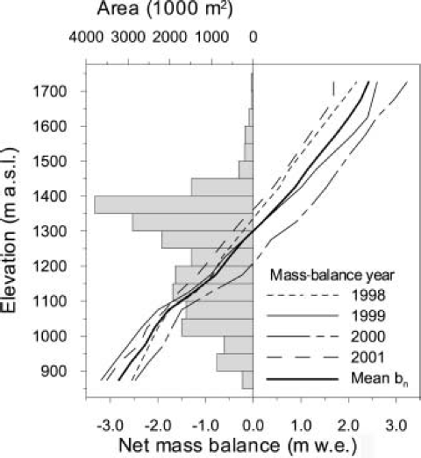
Fig. 2. The mass balance of Salajekna, 1998–2001, and the area– altitude distribution. The glacier is assumed to be at or near a balanced state.
Sensitivity analysis
Sensitivity analysis of the models to perturbations in input parameters shows the relative importance of different snowpack properties on SAR backscatter. The sensitivity tests for the Kirchhoff model show that the model is highly responsive to changes in dielectric constant across a range of possible values that are consistent with field measurements of dry snow (Fig. 3). The SPM is similarly sensitive to changes in the dielectric constant. The surface-scattering models parameterize surface roughness using the rms surface height and correlation length, and the height variation and width of that variation respectively. The models are sensitive to perturbations in these parameters, particularly when they are altered in combination.
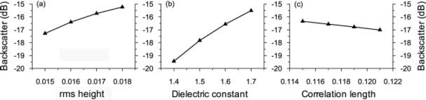
Fig. 3. Sensitivity analyses of the response of the Kirchhoff surface-scattering model to perturbations of rms height, dielectric constant and correlation length. The rms height and correlation length together describe the surface roughness. In each case, the non-perturbated parameters remained the same.
The Rayleigh model is sensitive to a combination of parameters describing individual scatterers and the dielectric slab they compose (Fig. 4). Grain radius, snow density, snow depth and the complex dielectric constant describe the volume as a homogeneous medium. The manipulation of the permittivity between 1.45 and 1.6 in the Rayleigh volume-scattering model (Fig. 4d) shows that the permittivity can influence the backscatter by about 2 dB for a dry snow cover (density 0.35 g cm–3; grain-size 0.5 mm; depth 3 m). These values represent the typical range of permittivity observed in the upper snowpack on Blåmannsisen and Salajekna in winter and early spring. Higher permittivity values are more representative of metamorphosed and/or wet snow. A permittivity of 1.7 would reduce the backscatter by a further 0.9dB to -26.5dB, while a permittivity of 1.8 results in a modelled backscatter of -25.6dB. The resultant model is found to be primarily dependent on perturbations of grain-size. The correction for optical grain-size reduces the backscatter from large-grained, dense firn, but increases backscatter in lower-density snow. The case shown in Figure 4a covers a range of values from the moderately sized snow grains (0.5 mm radius) to large crystals (1.25 mm radius), with a resultant 12 dB difference in backscatter (the difference is the same for physical and optical grain-sizes, though the latter results in a 2 dB increase in backscatter). Our qualitative observations of snow on the two glaciers suggest grain-sizes vary from 0.5 to 1 mm. This is supported by grain-size estimates from photographs taken of the snow and firn cores. In the absence of measurements, we have assumed a linear grain-size change associated with snow densification. At densities of <0.3gcm–3 a physical grain radius of 0.5 mm was assumed, rising to 0.66 mm for densities between 0.3 and 0.4gcm–3, and to 0.75 mm between 0.4 and 0.5gcm–3, while at densities of >0.5gcm–3 a physical grain radius of 1 mm was assumed. This assumption may introduce an error of ±3.3 dB (density 0.3 gcm–3; permittivity 1.533) for fine snow with grain-sizes of 0.5 ± 0.1 mm; for denser snow the error may be ± 2 dB (density 0.46gcm-3 ; permittivity 1.882). Such a linear grain-size distribution is a simplification. However, data series reported by Reference KeelerKeeler (1969) from Alta, Utah, USA, and by Reference Alley, Bolzan and WhillansAlley and others (1982) and Reference Shoji, Mitani, Horita and LangwayShoji and others (1993) from Antarctica indicate that linear grain-size and depth measurements occur. Density and depth are positively correlated, suggesting our assumption may not be unreasonable.
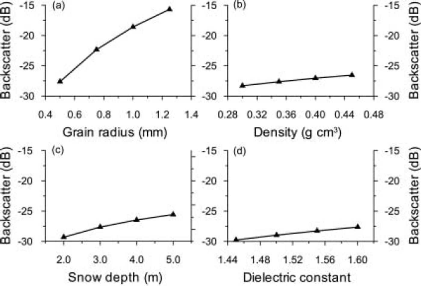
Fig. 4. The sensitivity of the Rayleigh volume-scattering model to perturbations in grain radius, density, snow depth and dielectric constant. At higher densities (>0.6 g cm–3) the optical grain-size correction reduces the influence of grain-size. The other parameters in each sensitivity test remained unchanged.
The correction for the optically equivalent grain-size (Reference Shi, Davis and DozierShi and others, 1993; Reference Forster, Jezek, Bolzan, Baumgartner and GogineniForster and others, 1999) dampens the sensitivity of the model to grain-size, with the aim of replicating in dense media the coherent scattering that reduces the backscatter. For low-density snow, incoherent scattering is enhanced, resulting in higher backscatter; the difference can be >3dB for a 0.5 m layer of fine powder snow. Above densities of around 0.6gcm–3 the correction reduces backscatter. This correction ameliorates the model’s tendency to be dominated by volume scattering from large-grained, dense layers such as firn.
By assuming hypothetical snowpacks with identical density profiles and perturbating the upper surface, we can see the impact of mass change on the volume scattering of the accumulation area. A 3.5m deep snowpack with a gradual density increase and stepped grain-size increases from 0.5 mm to 1 mm radii produced volume scattering of –15.52dB. Reducing the snowpack by removing the uppermost 0.5 m (density 0.28 g cm–3; grain radius 0.5 mm; permittivity 1.49) lowered the backscatter to –15.60 dB. Removing another layer (thickness 0.5 m, density 0.32 g cm–3; grain radius 0.5 mm; permittivity 1.57) reduced the backscatter to –15.87 dB. Removing a dense layer 0.5 m thick (density 0.48gcm–3; grain radius 0.75 mm; permittivity 1.93) from the hypothetical snowpack lowered backscatter to –18.01 dB.
Coupling the volume- and surface-scattering models, we can see the impact of changes in the dielectric contrast at the air–snow interface. This resulted in backscatter of –8.61, –8.36, –8.50 and –9.00 dB for the different snow-pack states described above. That backscatter is smaller in the first case (–8.61 dB) than the second and third cases, despite additional mass, shows the importance of the dielectric contrast at the air–snow interface. In this case, fresh powder snow, with small grains and a low density, reduces the surface scattering and total backscatter. These hypothetical cases show that small temporal fluctuations in mass balance would have a negligible or undetectable impact on backscatter. Changes in snow metamorphosis and internal storage of meltwater can have a stronger backscatter effect than the addition or loss of fresh, finegrained snow (Reference Rott, Sturm and MillerRott and others, 1993).
Observed backscatter from the firn area is typically between − 3 and − 6 dB . Lower volume scattering below the firn edge results in backscatter ranging from − 8 to -16dB. Backscatter during dry snow conditions is from the underlying firn or, below the firn limit, the glacier ice surface. Equation (3) shows that, for smoother surfaces modelled by the SPM, incidence angles must be small (<158) to promote scattering greater than -15dB. Even assuming a very rough snow surface (e.g. small wind features and a granular surface), the surface scattering accounts for <20% of the backscatter at incidence angles of 20-40˚. Kirchhoff scattering from the snow-ice interface is more important below the firn limit. Volume scattering from the firn accounts for around 70% of the total backscatter above the equilibrium-line altitude (ELA) or firn limit.
Backscatter response to changes in mass balance
The Salajekna mass-balance data indicate a fluctuation from net (specific) ablation of ∼0.5 m w.e. in 1998 and 1999 to a slight positive balance in 2000 before a strong negative balance again in 2001. Volume scattering in those years was estimated to be -15.70, -15.58, -15.09 and -17.61dB, respectively (at 1150ma.s.l.). The maximum variation was ∼2.5dB between years, with just less than 1 mw.e. net surface balance difference. This is due, in part, to the effect of slight surface melting in the 2000 data (as measured in situ) reducing the volume scattering in those data. Adding the surface-scattering model and scattering from glacier ice (below the ELA), the backscatter differences between years are <1 dB, suggesting only extreme variations in net balance can be detected (assuming uniform surface scattering).
Observed vs modelled backscatter
Digital values (β˚) were extracted from seven locations in the firn area and nine in the ablation area of the two glaciers; each sample represented a mean of 625 pixels from 25 × 25 pixel windows (Fig. 5). Sampling a large number of pixels reduces the potential impact of speckle, local topographic features or scatterers such as crevasses, and improves the calibration certainty in the SAR imagery (Reference Laur, Meadows, Sanchez and DwyerLaur and others, 1993). The locations were the same in all images and selected for homogeneity of backscatter in order to eliminate extreme topographic effects such as layover or severe foreshortening. The modelled backscatter for the two years with SAR data at the end of the accumulation season, 2000 (10 May) and 2001 (24 April), was calculated as –8.11 and –8.83 dB respectively. The observed backscatter below the ELA was –7.47 and –10.63dB (at the observation point closest to the mass-balance stakes). An ELA transect extracted from the 9 April 2001 scene exhibits very low backscatter immediately below the firn limit. The region of low backscatter (–15 dB) is confined to the region below the firn limit on Salajekna (Fig. 6) and parts of Blåmannsisen. It is likely that the reduction in backscatter is caused by the release of liquid water from the firn reservoir (it is too localized to be surface water). Mean hourly temperature data from a nearby weather station suggest temperatures around –6 to –9˚C. Two days prior to the image acquisition, temperatures were close to 0˚C. Both the lag time and the mechanism (water release from the firn or firn–ice transition) have been observed on other glaciers (Reference SchneiderSchneider, 2001). In the case of the two dates with SAR overpasses and contemporary field data (and dry snow conditions), the difference between modelled and observed backscatter was in the range 0.27–5.03 dB (four observations from Salajekna) and averaged 2.62 dB. The modelled backscatter in the firn area was within the calibration error of the observed SAR values (–2.93 to –5.92 dB); the firn models used firn profiles of 8 and 12 m thickness.
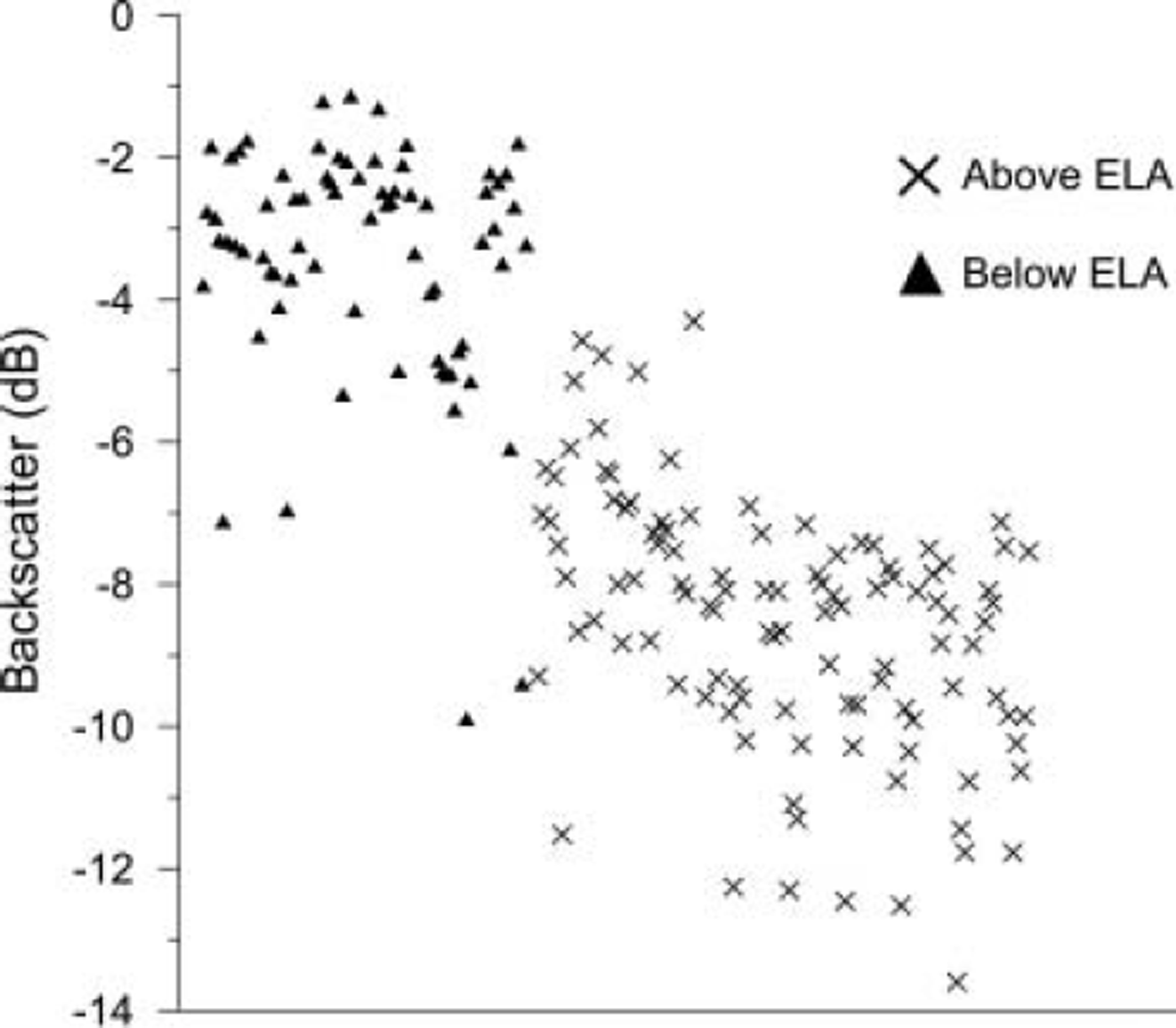
Fig. 5. The observed backscatter of 16 samples from each SAR image. The separation between bare-ice zone and firn area is largely clear, excepting a few outliers. These can be explained by perturbations in surface scatter at the snow–ice interface and by the occurrence of surface melting. The x axis represents the sampling order.
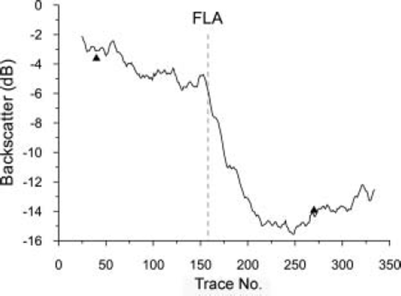
Fig. 6. A backscatter transect from the firn area of Salajekna to the bare-ice facies in the ablation area. The image from which the values were extracted was an ST2 image from 9 April 2001 which exhibited the presence of liquid water at the base of the snowpack. The x axis shows the location along the transect in pixels (which are 12.5 × 12.5 m). FLA is firn-line altitude.
Discussion
Snow probing suggests that significant local variation in accumulation rate and net balance may affect SAR backscatter. However, this is likely to be most pronounced above the firn limit, where volume scatter is most important. Excluding images with wet snow and an anomalous image from November 2000 which was lacking a header file and hence was uncalibrated, observed backscatter above the firn limit varies by 4.02 dB (n = 65), with a mean of -2.8 dB and a standard deviation of 1.0 dB. This variance can be explained by the GPR measurements made in 1998 which indicate that firn thickness varies by as much as 10 m on Blåmannisen and is mostly 10-15 m. The backscatter model estimates the total backscatter for two occasions when contemporaneous field data were available (10 May 2000 and 24 April 2001) to be within <1 dB in the 2000 dataset and 2.4 dB in the 2001 dataset (ablation area). In the accumulation area, firn dominates the backscatter and field data were not available to study annual changes in firn mass. A typical ‘winter balance’ (late-spring) snowpack was extrapolated and modelled using all field data. The model results for bare-ice facies overestimated backscatter by around 1-2 dB, suggesting either surface scatter from the air-snow interface or the snow-ice interface was exaggerated. Occasionally the difference between modelled and observed backscatter is larger (e.g. for scenes acquired in late April). It is likely that liquid water causes absorption in the snowpack on these occasions (Fig. 7). In the bare-ice facies the average backscatter was -8.19 dB, with a standard deviation of 1.54dB (n = 99).
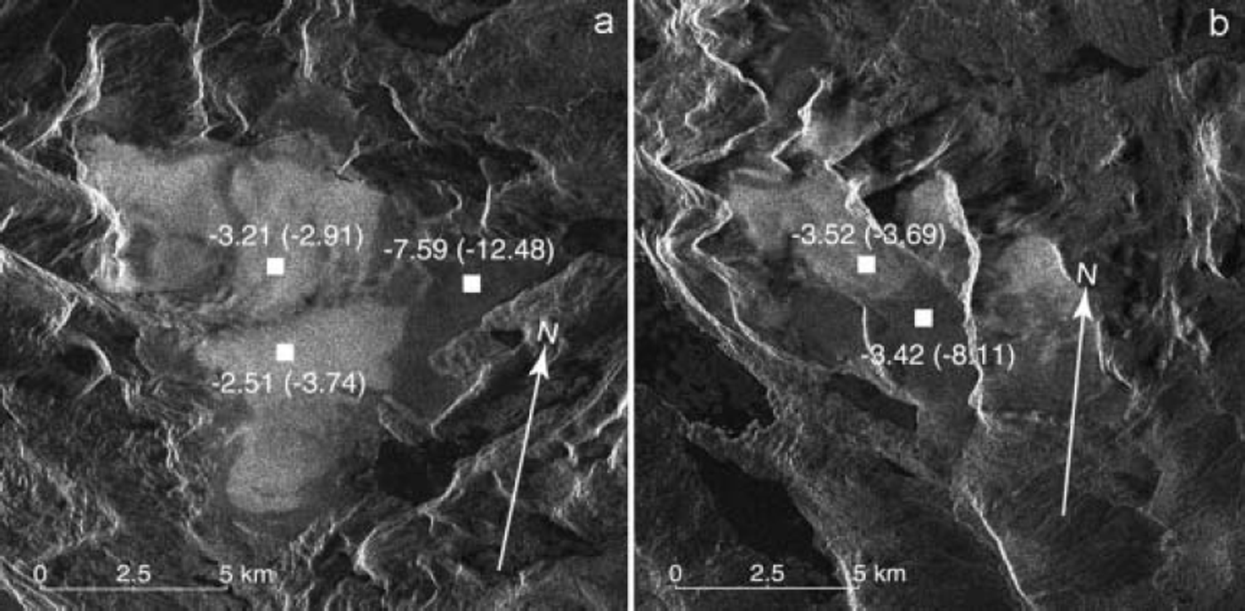
Fig. 7. SAR image subsets of Blåmannsisen (a) and Salajekna (b). The images are annotated with the 10 May 2000 observed and modelled (in parentheses) backscatter.
The inclusion of ∼ 2 % liquid water reduces the estimated backscatter to − 13 dB which is within 2 dB of the observed backscatter. The most significant anomaly is the high backscatter values retrieved from the bare-ice facies on Blåmannisen in the image acquired on 22 February 2002. Here backscatter from below the firn limit averages -4.6 dB which is typical of volume scattering from firn. The imagery indicates bright scattering across the bare-ice facies, suggesting a roughened snow surface or higher backscatter from the snow-ice interface. Snow-pit observations suggest that the ice surface is usually smoother in winter than in summer. It is possible that in late summer 2001 the roughened glacier surface was not in-filled by refrozen meltwater and consequently exhibited the strong surface scattering observed on summer snow-free glacier surfaces (e.g. Reference Brown, Kirkbride and VaughanBrown and others, 1999). Similar processes have been hypothesized by Reference Engeset, Kohler, Melvold and LundénEngeset and others (2002) for glaciers in Svalbard. Alternative processes resulting in higher backscatter include the formation of depth hoar, which, with large snow grains and moderate to low snow density, would volume-scatter strongly due to the relatively large spaces between grains (Reference Rott, Sturm and MillerRott and others, 1993; Reference Shi, Davis and DozierShi and others, 1993). Very strong surface scattering at the air–snow interface could also be responsible. The latter is less likely, as the modelling already assumes a very rough snow surface.
Backscatter modelling suggests that only large variations in winter balance should be detectable. Surface scattering at the snow–ice interface could affect the total backscatter more strongly if the hypothesis of Reference Engeset, Kohler, Melvold and LundénEngeset and others (2002) is correct. Interannual variations in net balance on the order of 0.5 m w.e. were measured on Salajekna; modelling suggests this variation is likely to result in a backscatter difference of <1 dB. Reference Forster, Jezek, Bolzan, Baumgartner and GogineniForster and others (1999) report an inverse correlation between backscatter and accumulation rate in the dry-snow facies on the Greenland ice sheet, suggesting small-scale differences in volume scattering can be detected. Modelling indicates that a perturbation in permittivity on the order of 0.2 (from 1.6 to 1.4), representing the difference between older, denser snow and fresh fine-grained snow, reduces backscatter from –16.6dB to –19.4 dB (assuming a rough snow surface and 23˚ incidence angle). This result shows that fresh powder snow will dampen surface scattering as a result of a lower dielectric contrast. This difference is likely to be enhanced by also reducing surface roughness (to values outside the validity range of our models).
Our measurements and those of Reference Forster, Jezek, Bolzan, Baumgartner and GogineniForster and other (1999) were made during dry snow conditions. Densification of the snow and firn during wet snow conditions cannot be observed using SAR imagery because liquid water will absorb microwaves and limit penetration. SAR must therefore be limited to winter balance observations or net balance observations in winter imagery. Reference Forster, Jezek, Bolzan, Baumgartner and GogineniForster and others (1999) note that, in Greenland, the differences in accumulation rate observed in the SAR backscatter variation are quite small and may be exceeded by the calibration uncertainty. This therefore limits the potential of any relationship between backscatter and accumulation rate in terms of absolute monitoring.
Conclusions
Our modelling and SAR observations show that spatial and temporal variations in surface roughness and grain-size distribution can mask the variance in SAR backscatter associated with mass-balance fluctuations. On glaciers with large spatial variations in snow accumulation and firn depth, backscatter above the firn limit may vary considerably, further complicating the retrieval of representative observations. We have shown that some observed changes in SAR backscatter are the product of metamorphism of the snow column rather than changes in mass. Near-field effects mean that there is no simple relationship between backscatter and snow density. A possible inverse relationship between backscatter and accumulation rate under dry snow conditions may exist, but this is not directly related to glacier mass balance but rather snow surface roughness and dielectric contrast. Furthermore, SAR data are not able to measure such fluctuations during melting conditions. Therefore net surface balance cannot be retrieved directly from SAR imagery over temperate glaciers. Nevertheless, we have shown that backscatter modelling, based on field measurements, enables us to better interpret the processes affecting SAR backscatter, decompose the backscatter into its component parts and infer processes extending beyond the period of in situ data. Proxy measurements may be retrieved and correlated to net surface parameters such as net surface balance or winter balance.
Acknowledgements
We thank the Swedish National Space Board for supporting this research and conference attendance. Additional funding was received from Ájtte’s Research Fund, the Andrée Foundation, Axel Hamberg’s Foundation, Göran Gustavsson’s Foundation, Lars Hierta’s Foundation and the Swedish Tourist Association’s Research Fund. Our data were provided by the Alaska Satellite Facility (ASF); we used their STEP software. We are grateful for their support and, in particular, help from the User Services Office at ASF. Our field assistants and logistic support are gratefully acknowledged, in particular the Olsen family in Sulitjelma. We also thank G. Hamilton and an anonymous reviewer for their comments.


