


1. Introduction
Since the late 1970s, numerical modelling has become established as an important technique for the understanding of ice-sheet dynamics. Ice-sheet models are particularly relevant for predicting future changes of ice sheets, mass loss and resultant contribution to sea-level rise in response to climate change (e.g. Reference Blatter, Greve and Abe-OuchiBlatter and others, 2011). Approximately half the mass transfer from the Greenland ice sheet to the surrounding ocean is by surface melting and runoff, while most of the rest is through ice streams and outlet glaciers that have a higher velocity than the surrounding ice (e.g. Reference Thomas, Bamber and PayneThomas, 2004). Since in many cases they form due to the existence of subglacial troughs, bed topography plays an important role in properly modelling the dynamics of the Greenland ice sheet. However, these trough systems typically have a width of <10 km and are thus poorly resolved in large-scale simulations that employ coarser grids.
The widely used digital elevation model (DEM) of the present-day bed topography of the Greenland ice sheet by Reference Bamber, Layberry and GogineniBamber and others (2001) has a grid spacing of 5km. However, many subglacial troughs are not well represented in this DEM, partly because their dimension is of the same order of magnitude as the grid spacing, partly because accurate data describing their detailed topographies were not available at the time when the DEM was assembled. With respect to the latter problem, the situation has meanwhile improved, and Reference Herzfeld, Wallin, Leuschen and PlummerHerzfeld and others (2011, Reference Herzfeld, Fastook, Greve, McDonald, Wallin and Chen2012) devised an algorithm for preserving important sub-scale morphologic characteristics at grids of lower resolution, in particular for linear features, such as canyons and ridgelines. The algorithm employs topological and mathematical morphological concepts to calculate canyon depth and ensure simple connectedness of canyons and canyon systems. The trough–bed algorithm was applied to derive a 5 km bed DEM, using new radar data collected by the Center for Remote Sensing of Ice Sheets (CReSIS, University of Kansas, USA) for Jakobshavn Isbræ and Helheim, Kangerdlussuaq and Petermann glaciers and integrated into the basic topography of Reference Bamber, Layberry and GogineniBamber and others (2001) outside those four regions (‘JakHelKanPet DEM’).
Comparing the different responses of two Greenland ice-sheet models, UMISM (University of Maine Ice Sheet Model; Reference FastookFastook, 1993; Reference Fastook and PrenticeFastook and Prentice, 1994) and SICOPOLIS (SImulation COde for POLythermal Ice Sheets; Section 2), both run at 5km resolution, between the original bed of Reference Bamber, Layberry and GogineniBamber and others (2001) and the more accurately represented JakHelKanPet bed, revealed significant differences in modelled surface velocity, basal water production and ice thickness. Consequently, modelled ice volumes for the Greenland ice sheet are significantly smaller for the JakHelKanPet DEM than for the Reference Bamber, Layberry and GogineniBamber and others (2001) DEM (Reference Herzfeld, Fastook, Greve, McDonald, Wallin and ChenHerzfeld and others, 2012). In this study, the model SICOPOLIS is applied to the Greenland ice sheet with resolutions ranging from medium (20 km) to high (5 km). The highest resolution makes full use of the JakHelKanPet bed, while for the lower resolutions the JakHelKanPet bed is downsampled by averaging the bed topography over the respective gridcells with 10 or 20 km edge length, which broadens and flattens the troughs. Within the framework of the SeaRISE (Sea-level Response to Ice Sheet Evolution) community effort (http://tinyurl.com/srise-umt), we discuss the impact of horizontal resolution on the simulated surface velocity field of the present-day ice sheet, and investigate the consequences for predictions of mass loss and contribution to sea-level rise under several climate-change scenarios for the next centuries.
2. Ice-Sheet Model Sicopolis
SICOPOLIS is a three-dimensional, polythermal ice-sheet model that was originally created by Reference GreveGreve (1995, Reference Greve1997) in a version for the Greenland ice sheet, and has been developed continuously since then (for the open-source version 3.0, used here, see sicopolis.greveweb.net). It is based on finite-difference solutions of the shallow-ice approximation for grounded ice (Reference HutterHutter, 1983; Reference MorlandMorland, 1984) and the shallow-shelf approximation for floating ice (Reference Morland, Van der Veen and OerlemansMorland, 1987; Reference MacAyealMacAyeal, 1989); the latter is not relevant for the Greenland ice sheet.
In this study, we use the regularized Glen flow law for the ice fluidity (inverse viscosity), 1 =r\, in the form of Reference Greve and BlatterGreve and Blatter (2009),

where T is the temperature relative to pressure melting (more precisely, following Reference Greve and BlatterGreve and Blatter, 2009, T = T — Tm + T0, where T is the ice temperature (K or 8C), Tm = T 0 — ft
p the pressure-dependent melting point, p the pressure, /3 the Clausius-Clapeyron gradient and T 0 the melting temperature at standard atmospheric pressure), A(T’) the rate factor, 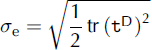 the effective stress (square root of the second invariant of the deviatoric stress tensor tD ) , f(ere) the creep function and E the flow enhancement factor. The rate factor is expressed in the form of an Arrhenius law,

with A0 the pre-exponential constant, Q the activation energy, R the universal gas constant and with T in kelvin. The creep function is given by a power law with an additional constant term,

with n the stress exponent and a0 the residual stress. In temperate ice, the rate factor of Eqn (2) is replaced by a rate factor, At, depending on the water content, W,

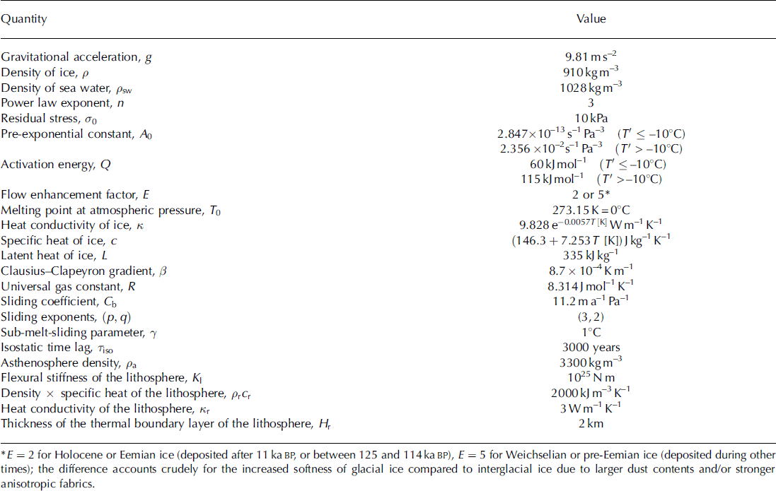
(Reference Lliboutry and DuvalLliboutry and Duval, 1985). The values for the several parameters largely follow the recent recommendations by Reference Cuffey and PatersonCuffey and Paterson (2010) and are listed, among others, in Table 1.
Table 1. Physical parameters used for the simulations in this study
Basal sliding under grounded ice, vb, is described by a Weertman-type sliding law with sub-melt sliding, of the form applied to the Greenland ice sheet by Reference Greve, Saito and Abe-OuchiGreve and others (2011),

where p and q are the sliding exponents, C b the sliding coefficient, 7 the sub-melt-sliding parameter, Tb the basal drag (shear stress), Nb the basal normal stress (counted positive for compression) and T^ the basal temperature relative to pressure melting (in 8C, always <08C ). Note that in the shallow-ice approximation the basal normal stress is equal to the hydrostatic pressure and the basal drag is equal to the hydrostatic pressure times the surface slope (e.g. Reference Greve and BlatterGreve and Blatter, 2009). Isostatic depression and rebound of the lithosphere due to changing ice load is modelled by the elastic-lithosphere-relaxing-asthenosphere (ELRA) approach (Reference Le Meur and HuybrechtsLe Meur and Huybrechts, 1996; Reference Greve, Straughan, Greve, Ehrentraut and WangGreve, 2001).
The model domain covers the entire area of Greenland and the surrounding oceans, projected on a polar stereographic grid with standard parallel 71 8N and central meridian 398W. Distortions due to this projection are accounted for as metric coefficients in all model equations. The present geometry (surface and basal topographies, ice thickness, equilibrated bedrock elevation) is derived from the ‘Greenland Developmental Data Set’ (Greenland_5km_ dev1.2.nc) provided on the SeaRISE website, which is complemented by the JakHelKanPet bed (that includes improved troughs for Jakobshavn Isbræ, Helheim, Kanger-dlugssuaq and Petermann glaciers; Reference Herzfeld, Wallin, Leuschen and PlummerHerzfeld and others, 2011, Reference Herzfeld, Fastook, Greve, McDonald, Wallin and Chen2012) and resampled to horizontal resolutions of 5, 10 and 20 km. In the vertical direction, sigma coordinates are used; the cold ice column, the temperate ice layer (if present) and the thermal boundary layer of the lithosphere are mapped separately to [0,1] intervals. The cold ice column is discretized by 81 gridpoints (concentrated towards the base), the temperate layer by 11 equidistant gridpoints and the thermal lithosphere layer by 41 equidistant gridpoints. Time-steps are 0.1-0.2 years for 5 km, 1 year for 10 km and 1-5 years for 20 km resolution.
3. Model Experiments
3.1. Paleoclimatic spin-up
In order to obtain a suitable present-day configuration of the Greenland ice sheet, it is desirable to carry out a paleo-climatic spin-up over at least a full glacial cycle. However, it is very difficult to reproduce the observed geometry by an unconstrained, freely evolving simulation without heavy tuning (e.g. Reference Greve, Saito and Abe-OuchiGreve and others, 2011). For this reason, we largely follow Reference Sato and GreveSato and Greve (2012) for the Antarctic ice sheet and carry out the spin-up simulation in four steps, each run using the result of the previous run as the initial condition:
-
1. An initial relaxation run with freely evolving ice topography over 100 years, starting from the present-day geometry and isothermal conditions at –108C everywhere, in order to avoid spurious noise in the computed velocity field (Reference CalovCalov, 1994). The ice sheet is not allowed to extend beyond its present-day margin. The surface temperature and the sea level are those of today; the surface mass balance and basal sliding are set to zero.
-
2. A steady-state run from 250 ka BP (kaBP means thousand calendar years before present (1989)) until 125 ka BP, with the entire topography (surface, bed, ice margin) kept fixed over time. The surface temperature is that of 125 kaBP; the surface mass balance is unspecified (due to the fixed topography). The purpose of this run is to bring internal and basal temperatures to near equilibrium for the climate conditions at 125 ka BP.
-
3. A transient run from 125 ka BP until 100 years BP; with the entire topography kept fixed over time in order to enforce a good fit between the simulated and observed present-day topographies. The surface temperature varies over time (see below); the surface mass balance is unspecified.
-
4. A short transient run from 100 years BP until the present, with evolving ice topography in order to avoid transition shocks at the beginning of the subsequent future-climate experiments. The climatic forcing (surface temperature, surface mass balance) and the sea level are kept steady at today’s conditions, and the ice sheet is not allowed to extend beyond its present-day margin.
This procedure is followed for 10 and 20 km resolution. However, in order to limit the required computation time, the spin-up for 5 km resolution is conducted from 5 ka BP until today only, with the resolution-doubled output of the 10 km version of run 3 at 5 ka BP as the initial condition. Over the first 10 years (until 4.99 ka BP), the topography (surface, bed, margin) is changed gradually to the result of the 5 km version of run 1, and from then on the procedure is as above (run 3 until 100 years BP, followed by run 4 until the present).
Apart from the fixed geometry of the ice sheet in runs 2 and 3, the runs are conducted with the forcings suggested by SeaRISE. The mean annual and mean July (summer) surface temperatures, Tma and Tmj, respectively, are decomposed into present-day spatial distributions plus a time-dependent anomaly, AT(t):

where t is time, h surface elevation, <p geographical latitude and A geographical longitude. The present-day parameterizations are by Reference Fausto, Ahlstrøm, Van As, Bøggild and JohnsenFausto and others (2009):

where temperatures are in 8C, surface elevations in km a.s.l., latitudes in 8 N and longitudes in 8W (counted positive). The time-dependent anomaly, AT(t), results from the Greenland Ice Core Project (GRIP) oxygen isotope (d18O) record (Reference DansgaardDansgaard and others, 1993; Reference JohnsenJohnsen and others, 1997), converted to temperature with a AT / d18O conversion factor of 2.48C %–1 (standard value used by Reference HuybrechtsHuybrechts, 2002). The resulting temperature anomaly is shown in Figure 1.
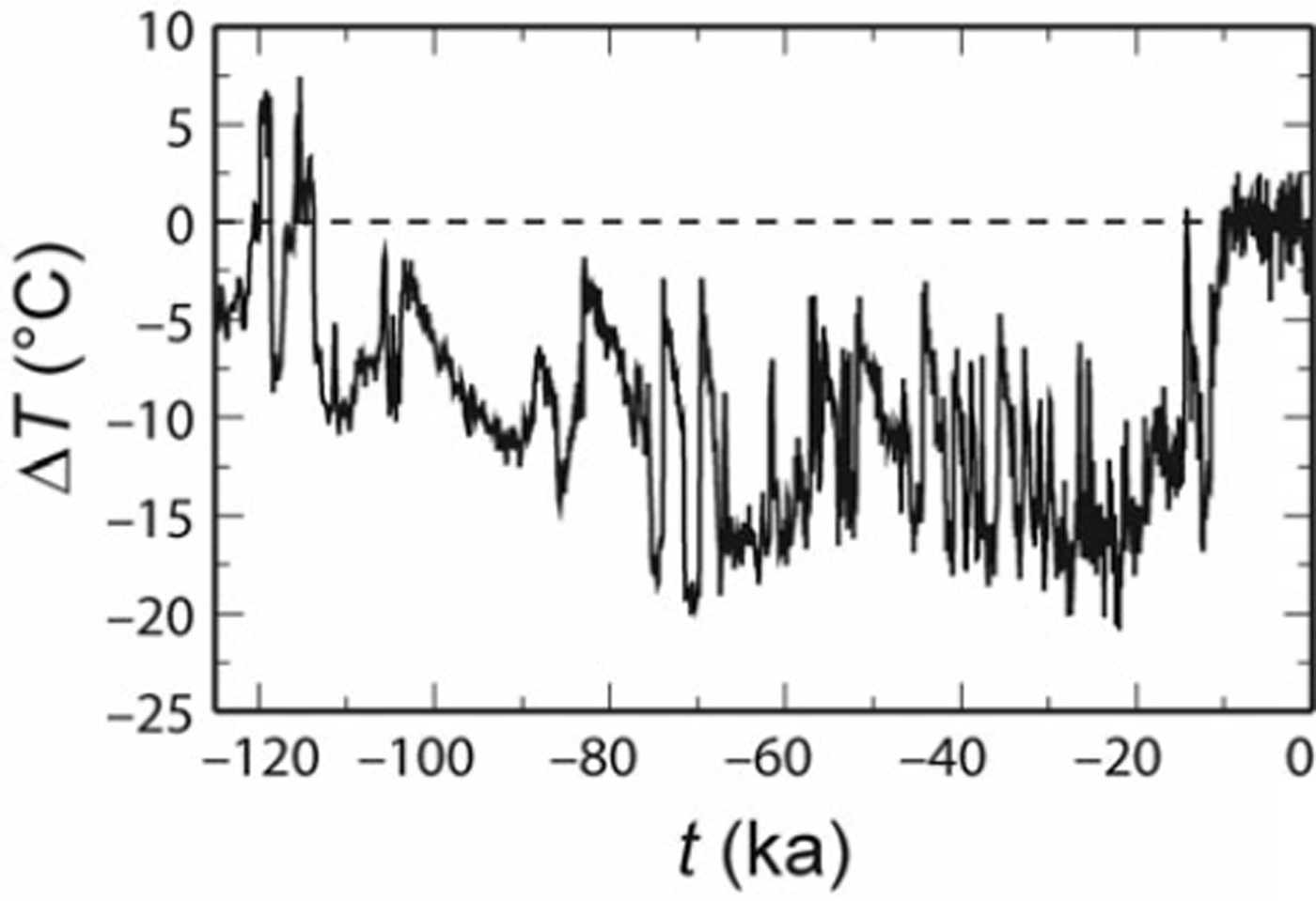
Fig. 1. Surface temperature anomaly, AT(t), derived from the GRIP d18O record (Reference DansgaardDansgaard and others, 1993; Reference JohnsenJohnsen and others, 1997).
Precipitation, surface melting and sea-level forcings are not required for runs 2 and 3 due to the fixed geometry approach. For run 4, the present-day mean annual precipitation data by Reference EttemaEttema and others (2009) are used, and they are converted to snowfall rates (solid precipitation) on a monthly basis using the empirical relation of Reference MarsiatMarsiat (1994). Surface melting is parameterized by Reference ReehReeh’s (1991) positive degree-day (PDD) method, supplemented by the semi-analytical solution for the PDD integral by Reference Calov and GreveCalov and Greve (2005). The PDD factors are /3ice = 8mmw.e. d–1 8C–1 for ice melt and Anow = 3 mm w.e. d–1 8C–1 for snowmelt (Reference Huybrechts and de WoldeHuybrechts and de Wolde, 1999). Furthermore, the standard deviation of short-term, statistical air temperature fluctuations is er = 58C, and the saturation factor for the formation of superimposed ice is chosen as Pmax = 0:6 (Reference ReehReeh, 1991).
As for the geothermal heat flux, we deviate from the recommendation of SeaRISE and use a slightly modified version of the map by Reference GreveGreve (2005, right panel of his fig. 4) instead. It is an interpolation based on the global heat-flux representation by Reference Pollack, Hurter and JohnsonPollack and others (1993) and prescribed point values at the deep ice-core locations GRIP (59mWm–2 ) , NorthGRIP (135mWm–2 ) , Camp Century (54mWm– 2 ) and Dye3 (26mWm– 2 ) . These values were found to provide better agreements between simulated and observed ice thicknesses and basal temperatures at the ice-core locations for simulations with 10 km resolution than the values listed by Reference GreveGreve (2005) that were determined on the basis of simulations with 20 km resolution (Greve, unpublished imformation).
The simulated present-day configuration of the ice sheet (result of run 4) is used as the initial condition for the future-climate experiments described in the following subsection.
3.2. Future-climate experiments
For the future-climate experiments, we use the following subset of the suite defined by SeaRISE (Reference BindschadlerBindschadler and others, 2013):
Experiment CTL: constant climate control run; beginning at present (more precisely, the year 2004, corresponding to t = 0) and running for 500 years, holding the climate steady to the present climate.
Experiment C2: 1.5 x AR4 climate forcing (mean annual temperature, mean July temperature and precipitation anomalies derived from an ensemble average from 18 of the Intergovernmental Panel on Climate Change’s Fourth Assessment Report (IPCC AR4) models, run for the period 2004-98 under the A1B emission scenario; Reference Nakicenovic and SwartNakicenovic and Swart, 2000) until 2098, then held steady.
Experiment S1: constant climate forcing, 2 x basal sliding (implemented by doubling the value of the sliding parameter, C b , everywhere).
Experiment M2: constant climate forcing, 20mw.e. a∼1 ocean-induced marginal melting (applied at grounded ice cells that have a base below the sea level and are adjacent to ocean).
Experiment R8: combination experiment approximating IPCC’s RCP (Representative Concentration Pathway) 8.5 scenario (Reference MeinshausenMeinshausen and others, 2011; Reference Van VuurenVan Vuuren and others, 2011); 1.5 x AR4 climate forcing (continued beyond 2098 over the entire 500 years) plus 1.5 x basal sliding plus ocean-induced marginal melting increasing over time to a maximum of 70 mw.e. a∼1 (for details of this set-up and its rationale see Reference BindschadlerBindschadler and others, 2013).
The reason for the selection of C2, S1 and M2 is that, within the ‘2011 Sensitivity Experiments’ defined by SeaRISE, they are closest to the settings of the combination experiment R8. For all experiments, the present-day surface temperature, precipitation, conversion to snowfall (solid precipitation), surface melting and geothermal heat flux are as explained in Section 3.1. All experiments are carried out at the three different resolutions of 5, 10 and 20 km. In order to minimize the inconsistency that arises from the transition from the essentially fixed-topography spin-up to the future-climate experiments with evolving topography, in neither case is the ice sheet allowed to extend beyond its present-day margin (a test of the control run at 5 km resolution without this constraint showed an immediate ice area increase of ∼ 0:14 x 106 km2 or ∼ 8 . 5% of the initial area).
4. Results
The results of the paleoclimatic spin-up run at the highest resolution of 5 km (Section 3.1) for the present are shown in Figure 2. Comparison of the simulated (Fig. 2a) and observed (Fig. 2b; data by Reference Joughin, Smith, Howat, Scambos and MoonJoughin and others, 2010) surface velocities reveals that the general pattern with the low-velocity (<10ma∼1 ) ‘backbone’, the general acceleration towards the coast and the organization into drainage systems is reproduced very well. The most conspicuous discrepancy is in the region of the northeast Greenland ice stream (NEGIS), which appears only very weakly in the simulation.

Fig. 2. Results of the paleoclimatic spin-up at 5 km resolution. (a) Simulated (vs) and (b) observed (vs, obs; Reference Joughin, Smith, Howat, Scambos and MoonJoughin and others, 2010) present-day surface velocities. (c) Difference of simulated (H) and observed (Hobs) present-day ice thicknesses. (d) Simulated present-day basal temperature relative to pressure melting, Tb0 .
This is reflected in the difference of simulated and observed ice thicknesses (Fig. 2c). This misfit is generally small (<100m) due to the fixed-topography constraint during most of the spin-up run. However, some areas stick out, and one of them is the NEGIS area, where simulated ice thicknesses are too large as a consequence of the under-predicted drainage towards the coast. The same holds for the area of Petermann Gletscher in the northwest. In contrast, along the southeastern ice margin simulated ice thicknesses are generally too small, which may be due to over-predicted ice flow (difficult to judge because of gaps in the observational coverage) or to inaccuracies in the surface mass balance. Most of the rapid topographic adjustments that lead to these local misfits arise early during the short transient run 4 over 100 years at the end of the spin-up sequence. After these 100 years, the ice-sheet geometry has largely stabilized, and no spurious rapid adjustments occur in the future-climate runs (including the control run).
Basal temperatures (Fig. 2d) are at the pressure-melting point for ∼ 4 4% of the ice-covered area, including all major drainage basins. At the deep ice-core sites, GRIP, NorthGRIP, Camp Century and Dye3, the spin-up run produces basal temperatures of —8:66°C, —2:64°C (pressure-melting point), —13:96°C and —14:08°C, respectively, while the observed values are —8:56°C (GRIP; Reference DansgaardDansgaard and others, 1993; Reference Dahl-JensenDahl-Jensen and others, 1998), —2:4°C (NorthGRIP; Reference Dahl-Jensen, Gundestrup, Gogineni and MillerDahl-Jensen and others, 2003; North GRIP Members, 2004), — 13:00°C (Camp Century; Reference Dansgaard, Johnsen, Møller and LangwayDansgaard and others, 1969; Reference Gundestrup, Clausen, Hansen and RandGundestrup and others, 1987, Reference Gundestrup, Dahl-Jensen, Hansen and Kelty1993) and —13:22°C (Dye 3; Reference Gundestrup and HansenGundestrup and Hansen, 1984). The good agreement is mainly due to the choice of the geothermal heat flux, as explained in Section 3.1. Using the distribution by Reference Shapiro and RitzwollerShapiro and Ritzwoller (2004) that is recommended in the SeaRISE specifications worsens the agreement significantly (Reference Seddik, Greve, Zwinger, Gillet-Chaulet and GagliardiniSeddik and others, 2012).
To continue the analysis of surface velocities, Figures 3-6 show the simulated and observed (Reference Joughin, Smith, Howat, Scambos and MoonJoughin and others, 2010) distributions in the vicinity of Jakobshavn Isbræ, Helheim, Kangerdlugssuaq and Petermann glaciers for all three applied resolutions. For Jakobshavn Isbræ (Fig. 3), the 5 km run best reproduces the high flow velocities along the center line, while, as expected, the pattern is increasingly smeared out for 10 and 20 km resolution. A problem with the velocity field of the 5 km run is that the area of fast flow is too much focused on the narrow trough in the bed, while the observed field is somewhat wider. This is a consequence of the local nature of the shallow-ice approximation; similar simulations with the full Stokes model Elmer/Ice feature a wider fast-flowing area (Reference Seddik, Greve, Zwinger, Gillet-Chaulet and GagliardiniSeddik and others, 2012). An attempt to quantify the misfit between simulated and observed velocities is made in the scatter plots shown in Figure 3e–g. For all three resolutions, the slopes, m, of the least-squares regressions are less than unity, so that even for 5 km resolution fast ice flow is only partly captured by the simulation. However, the increasingly degraded ice-stream patterns for 10 and 20 km resolution are reflected well by the strongly decreasing values of m.
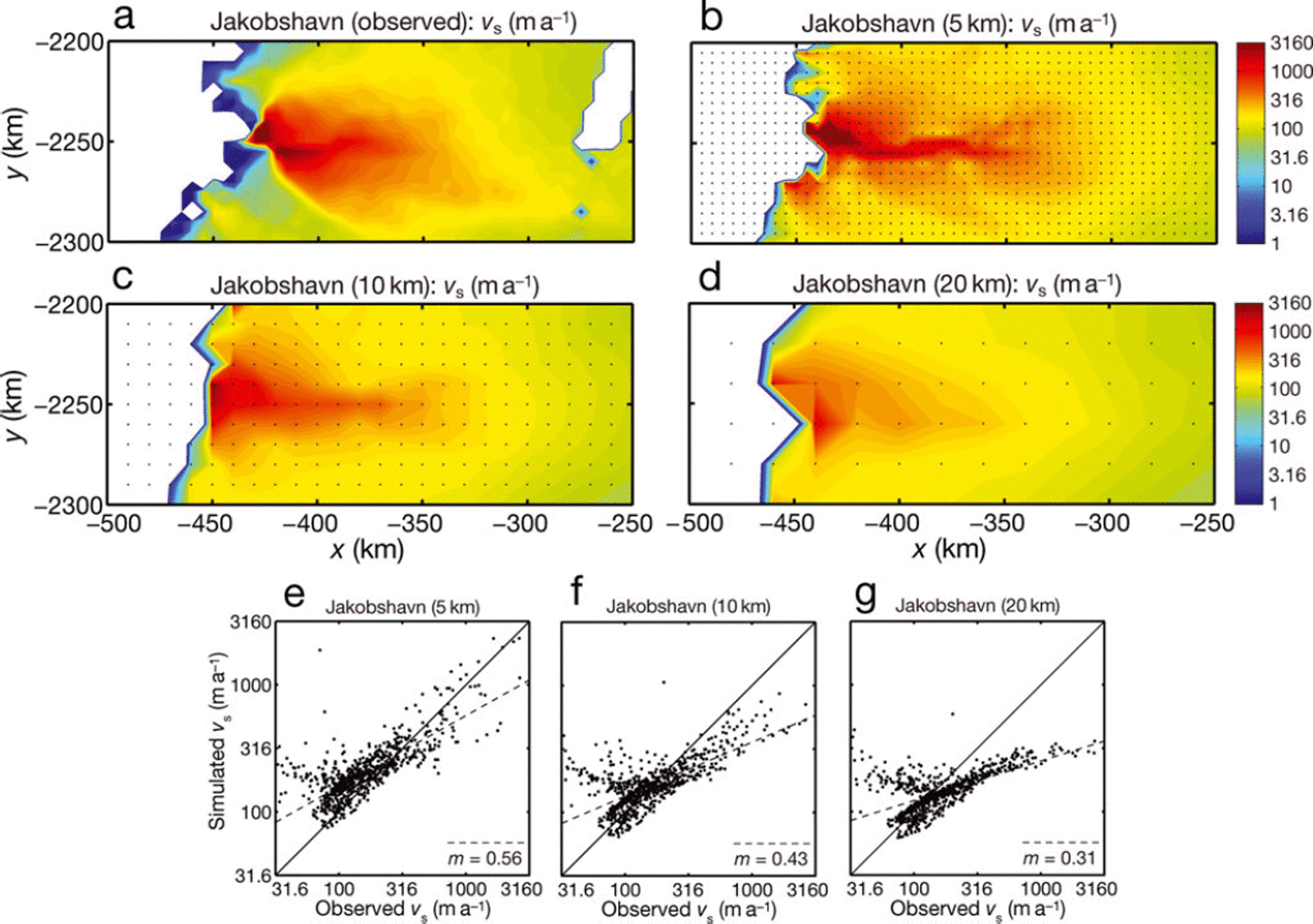
Fig. 3. Results of the paleoclimatic spin-ups for the vicinity of Jakobshavn Isbræ. (a–d) Present-day surface velocities: (a) observed (Reference Joughin, Smith, Howat, Scambos and MoonJoughin and others, 2010) and for simulated resolutions of (b) 5 km, (c) 10 km and (d) 20 km. (e–g) Scatter plots of simulated vs observed velocities for the three different resolutions (simulation data re-gridded to a uniform spacing of 5 km). Solid lines in the scatter plots are ideal lines (simulated = observed), dashed lines are least-squares regressions and m denotes their slopes.
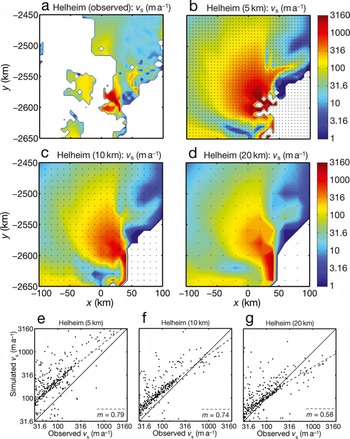
Fig. 4. Same as Figure 3, but for Helheim Glacier.

Fig. 5. Same as Figure 3, but for Kangerdlugssuaq Glacier.
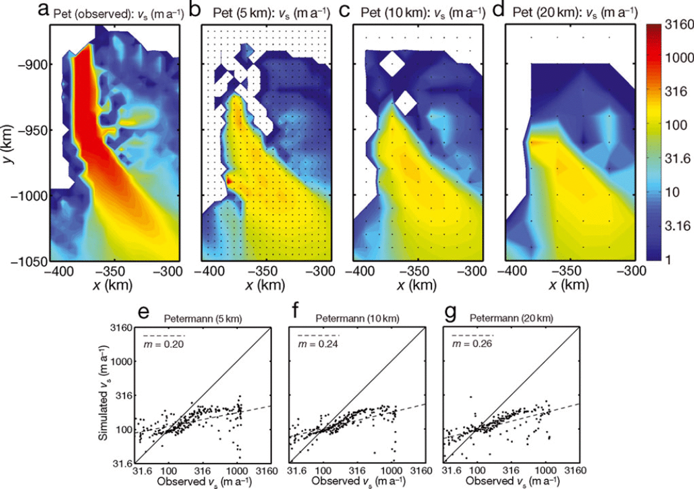
Fig. 6. Same as Figure 3, but for Petermann Gletscher.
For Helheim Glacier and its drainage area further upstream (Fig. 4), the observational data only cover the fastest-flowing area near the terminus. Analogous to the situation at Jakobshavn Isbræ, the observations are best matched by the 5 km run (which even resolves the nunataks near the ice margin), while the 10 and 20 km runs show less pronounced fast flow. In addition, the pattern of the velocities obtained at 5 km resolution agrees well with the pattern found in the balance velocities by Reference Bamber, Layberry and GogineniBamber and others (2001). The slopes, m, of the least-squares regressions in the scatter plots (Fig. 4e-g) are closer to unity than those for Jakobshavn Isbræ, and the values for 5 and 10 km resolution differ only slightly, while the value for 20 km resolution is distinctly smaller. The reason why the 10km simulation performs better for Helheim Glacier than for Jakobshavn Isbræ is that the drainage basin is wider, so it is better resolved by the 10 km grid than the more channelized Jakobshavn Isbræ.
The multiple-tributary structure of Kangerdlugssuaq Glacier (Fig. 5) is also reproduced well by the 5 km run and, to a lesser extent, by the 10 km run. In the 20 km run, the structure is only reflected rudimentarily, and fast ice flow limited to a few gridpoints near the terminus of the glacier. This is clearly corroborated by the scatter plots (Fig. 5e-g), which are similar to those for Helheim Glacier, with similar, close-to-unity regression slopes, m, for 5 and 10 km resolution and a much smaller value for 20 km resolution.
The situation is different for Petermann Gletscher (Fig. 6). None of the three resolutions reproduces adequately the very pronounced, ∼150km long fast-flowing zone of the observational data. Even for the 5 km run the modelled length of the fast-flowing zone is only about two-thirds of the actual length, and the velocities are far too small. An explanation for this mismatch lies in the fact that Petermann Gletscher had a ∼ 7 0 km long floating tongue that is not represented in the grounded-ice-only simulations. Furthermore, about a quarter of the ice tongue calved in 2010. In the simulations, the floating tongue hence appears partly as grounded and partly disintegrated. The poor agreement for all three resolutions is also evident in the scatter plots (Fig. 6e-g), which show regression slopes m < 0:26, much smaller than for Jakobshavn Isbræ and Helheim and Kangerdlugssuaq Glaciers.
Let us now investigate the influence of horizontal resolution on ice volume evolution for the future-climate experiments described in Section 3.2. Figure 7a, c, e and g show the absolute ice volumes (in meters sea-level equivalent; mSLE) for all five scenarios. The initial (t = 0, equivalent to the year 2004) spread of ice volumes is ∼10cmSLE and increases over time to ∼20cmSLE. Ice volumes are consistently smaller for higher resolutions and larger for lower resolutions because of the faster ice flow occurring in the high-resolution simulations.

Fig. 7. Results of the future-climate runs for horizontal resolutions of 5 km (solid lines), 10 km (dashed lines) and 20 km (dash-dotted lines). Ice volumes (a, c, e, g) and differences relative to the constant-climate control run CTL (b, d, f, h) for runs (a, b) C2 (1.5 x AR4 climate forcing until 2098, then held steady), (c, d) S1 (2 x basal sliding), (e, f) M2 (20mw.e. a∼1 ocean-induced marginal melting and (g, h) R8 (combination experiment, 1.5 x AR4 climate forcing (continued over 500 years) plus 2 x basal sliding plus up to 70mw.e. a∼1 ocean-induced marginal melting.
In contrast, the ice volume sensitivities of experiments C2, S1, M2 and R8 relative to the control run CTL (plotted in Fig. 7b, d, f and h as control minus experiment in order to have positive numbers) show only a small dependence on resolution. After 500 years, for experiment C2 (1.5 x AR4 climate forcing), the spread is ∼3.6cmSLE (spread/mean 12.4%), for S1 (2 x basal sliding) ∼4.1 cmSLE (spread/mean 19.0%), for M2 (20mw.e. a∼1 marginal melting) ∼3.1 cm SLE (spread/mean 55.4%) and for R8 (combination experiment) ∼6.4 cm SLE (spread/mean 2.5%). No consistent trend is found: for C2 and M2, the lowest resolution (20 km) produces the largest sensitivity, while for S1 and R8 the highest resolution (5 km) produces the largest sensitivity.
It is particularly noteworthy that the dependence of ice volume sensitivity on horizontal resolution is so small for the combined experiment R8 that includes forcings induced by surface climate, the surrounding ocean and ice-dynamical changes, and thus comes closest to a realistic scenario. This experiment produces an ice volume sensitivity of ∼2.5 m SLE after 500 years (more than one-third of the entire volume of the Greenland ice sheet), with, as listed in the previous paragraph, only 2.5% variation among the runs with 5, 10 and 20 km resolution. The main reason why the sensitivity of this experiment is so much larger than the combined sensitivities of C2, S1 and M2 is that the 1.5 x AR4 climate forcing is extrapolated beyond 2098 over the entire 500 year simulation time, while in C2 the climate forcing is held steady after 2098 (Section 3.2). This leads to a much stronger warming, and thus a more pronounced surface melting, in experiment R8 during the 22nd to 25th centuries.
5. Summary and Discussion
We have applied the dynamic/thermodynamic ice-sheet model SICOPOLIS to the Greenland ice sheet and carried out paleoclimatic spin-ups as well as a set of future-climate runs specified by the SeaRISE community effort. Three different resolutions were employed, ranging from medium (20 km) via medium-high (10 km) to high (5 km), and the fixed-topography approach in the spin-ups ensured a good match between the modelled and observed present-day ice sheet. Comparison of modelled and observed surface velocities for the four ice streams and outlet glaciers (Jakobshavn, Helheim, Kangerdlugssuaq, Petermann) with well-represented troughs in the bed topography showed, with the exception of Petermann Gletscher, reasonably good agreements for the 5 km spin-up, moderate agreements for the 10 km spin-up and rather poor agreement (ice flow too slow) for the 20 km spin-up.
In the future-climate experiments over 500 years, the simulated absolute ice volumes are consistently smaller for higher resolutions and larger for lower resolutions, with an initial spread of ∼-10cmSLE that increases over time to ∼20cmSLE. In contrast, the ice volume sensitivities of the different scenarios relative to the constant climate control run do not show a consistent dependence on resolution, and even for the most extreme combination experiment that leads to an ice loss of ∼2.5 m SLE after 500 years the spread for the three runs with different resolutions is limited to ∼6.4cmSLE (less for the three other scenarios). Consequently, for all considered forcings (surface climate, the surrounding ocean, ice-dynamical changes and a combination of them), most of the resolution dependence consists of an offset of the absolute ice volume, whereas ice volume sensitivities relative to the control run show a surprisingly small dependence on resolution.
Reference Herzfeld, Fastook, Greve, McDonald, Wallin and ChenHerzfeld and others (2012) reported a similar finding, where the constant climate control run CTL and the 2 x basal sliding run S1 were carried out with two different ice-sheet models (UMISM, SICOPOLIS) at 5 km resolution for the Reference Bamber, Layberry and GogineniBamber and others (2001) DEM and the JakHel-KanPet DEM (that is used here). For both models, the main effect of the improved DEM consisted of an up to ∼10cm SLE decrease in the simulated absolute ice volumes, while the sensitivities (S1 relative to CTL) were an order of magnitude lower. Together with the findings reported here, this relative insensitivity could indicate that, on multi-decadal to centennial (and longer) timescales, the mass transfer from the Greenland ice sheet to the surrounding ocean is not so much controlled as merely organized by the fast-flowing ice streams and outlet glaciers. Hence, reproducing every detail of their small-scale dynamics may not be imperative for capturing the essentials of the large-scale response of the ice sheet to climate change.
A limitation of this study is that the findings arose from a model (SICOPOLIS) that is based on the shallow-ice approximation. It is known that the shallow-ice approximation describes fast-flowing ice streams and outlet glaciers only in a very simplified way; their dynamics is modelled more appropriately by shelfy-stream, higher-order or even full-Stokes dynamics (e.g. Reference Kirchner, Hutter, Jakobsson and GyllencreutzKirchner and others, 2011). Models that employ different flavors of ice dynamics beyond the shallow-ice approximation exist (Reference PattynPattyn and others, 2008) and have been applied to real-world, large-scale ice-sheet dynamics (Reference Pollard and DeContoPollard and DeConto, 2009; Reference Ren, Fu, Leslie, Chen, Wilson and KarolyRen and others, 2011; Reference Larour, Seroussi, Morlighem and RignotLarour and others, 2012; Reference Seddik, Greve, Zwinger, Gillet-Chaulet and GagliardiniSeddik and others, 2012; Reference Winkelmann, Levermann, Frieler and MartinWinkelmann and others, 2012), but a systematic study of the influence of resolution on ice stream representation and ice volume evolution under future-climate scenarios has not been carried out so far (to the best of our knowledge). Hence, future work will have to show whether our findings still hold when ice streams and outlet glaciers are modelled by more sophisticated dynamics, or whether the latter must be necessarily combined with very-high to ultra-high resolutions (at least locally) in order to produce good results.
Acknowledgements
We thank R.A. Bindschadler, S. Nowicki and others for their efforts in the management of the SeaRISE project, J.V. Johnson and others for compiling and maintaining the SeaRISE datasets and F. Saito and A. Abe-Ouchi for continued, fruitful exchange on ice-sheet modelling issues. R. Greve’s invitation to the Workshop on Numerical Methods for Scale Interactions (Hamburg, Germany, 21–23 September 2011) by A. Humbert, T. Frisius and J. Behrens, which kicked off this study, is gratefully acknowledged. Thoughtful and constructive comments by the scientific editor, T.H. Jacka, and two anonymous reviewers helped to improve the manuscript considerably. This work was supported by the Japan Society for the Promotion of Science (JSPS) through a Grant-in-Aid for Scientific Research A (No. 22244058) to R. Greve, and by a NASA Cryospheric Sciences Award (NNX11AP39G) to U.C. Herzfeld.



