

Introduction
Recently developed numerical avalanche simulation tools, RAMMS (Rapid Mass Movements; Reference Christen, Kowalski and BarteltChristen and others, 2010b), SAMOS (Snow Avalanche MOdelling and Simulation; Reference Sampl and ZwingerSampl and Zwinger, 2004) and others (Reference Barbolini, Gruber, Keylock, Naaim and SaviBarbolini and others, 2000), are useful for avalanche engineers tackling problems involving hazard mapping, planning of mitigation measures or back-calculation of catastrophic avalanche events (Reference Christen, Bartelt and KowalskiChristen and others, 2010a). Such models can predict flow paths, run-out distances, deposition heights, velocities and impact pressures of snow avalanches in three-dimensional terrain. However, the results of these numerical models depend strongly on the quality of input information, such as release area, release height, forest information and the underlying digital elevation model (DEM). Although snow cover can smooth out some terrain effects, a detailed representation of the surface is essential for avalanche modeling. Especially in a complex topography containing bumps, depressions, ridges and gullies, the avalanche path alters, depending on characteristics of the DEM, such as spatial resolution, vertical accuracy and contained anomalies and artifacts. Caution is advised in resampling DEM data, because resampling can significantly change DEM characteristics such as slope, aspect and curvature (Reference Ahmadzadeh and PetrouAhmadzadeh and Petrou, 2001; Reference Dixon and EarlsDixon and Earls, 2009).
Since the 1960s, DEMs have been generated using airborne photogrammetry. The surface elevation can be calculated using two different looking angles within the visible or near-infrared part of the electromagnetic spectrum. Depending on the flying altitude of the sensor, spatial resolutions of ∼1m can be achieved with a vertical accuracy of some decimeters (ASPRS, 2001). However, to cover wide areas many flight-lines are necessary, increasing the costs. This methodology has a long tradition and is still widely used for topographic mapping all over the world. Novel digital optical scanners with enhanced radiometric resolution and improved automated data processing are becoming more and more important for DEM generation and further applications in alpine terrain. Therefore it is likely that digital photogrammetry will replace analog methods in the near future.
With the launch of spatially highly resolved optical satellite sensors, wide-area DEMs can be acquired from space. If a sensor can acquire data from at least two different viewing angles, such models can be generated. Depending on the spatial resolution of the sensor, elevation models with a spatial resolution of 30 m (e.g. Advanced Spaceborne Thermal Emission and Reflection Radiometer (ASTER)) down to 2 m (e.g. QuickBird) can be generated (Table 1). However, these sensors are limited by clouds, cast shadows and invisible areas in mountainous terrain, where no elevation information can be retrieved. No optical sensors, including aerial imagery, can penetrate vegetation cover such as forests. Therefore their DEM products show the surface of a canopy and are referred to as digital surface models (DSMs).
Synthetic aperture radar (SAR) radio detection and ranging sensors can acquire data through clouds and cover wide areas using microwaves. Radar is thus a promising tool for DEM generation, especially in cloudy areas like the tropics. In the past, the spatial resolution of such DEM products has been quite coarse. The Shuttle Radar Topography Mission (SRTM; Reference FarrFarr and others, 2007) was the first to cover large parts of the Earth’s surface with a spatial resolution better than 100 m and a vertical accuracy of ∼50 m. New SAR missions, such as TerraSAR-X (Reference Liao, Tian and XiaoLiao and others, 2007), provide a much better spatial resolution, <5m, as well as better vertical accuracies and therefore have great potential for future DEM generation purposes.
Light detection and ranging (lidar) technology was introduced in the late 1970s. This methodology uses laser beams to measure the distance between the sensor and the Earth’s surface. Because the beam is partly reflected by vegetation and partly by the ground below it, DSMs and digital terrain models (DTMs) can be generated using the first and the last reflection signal recorded. These two terrain representations can be used to accurately retrieve object heights (Reference Lillesand and Kiefer.Lillesand and Kiefer, 2008). Though the acquisition of airborne lidar data for wide areas is expensive, this methodology achieves the best spatial resolutions (down to 50 cm) and vertical accuracies (down to 10 cm).
We assess the sensitivity of numerical avalanche simulations to DEM quality and resolution by comparing the results of the different RAMMS simulations.We compare the flow paths, run-out distances, deposits, velocities and impact pressures. Table 1 provides an overview of important sensors for DSM and DTM generation, listing the spatial resolution and vertical accuracies of the products.
Test Sites and Investigated Digital Elevation Models
To assess the influence of DEM resolution and quality on numerical avalanche-modeling results, we use well-documented avalanche events from two test sites in Switzerland which have varying terrain characteristics.
Dorfberg: channeled slope characteristics
The Dorfberg area, located near Davos-Dorf, eastern Switzerland, has very diverse topographic characteristics. It ranges from the top of Salezer Horn (2536ma.s.l.) to the valley bottom covered by Davos lake at 1560 ma.s.l. (Fig. 1). Every year, numerous dry and wet snow avalanches occur on its southeast, exposed, 30–40˚ slopes. The very steep, ∼1km long Salezer gully often channels the flow of avalanches releasing at the steep southeastern slope of the Salezer Horn. A large wet snow avalanche occurred at the end of March 2008. Run-out distance and depositions were accurately documented using aerial imagery, helicopter-based lidar and GPS measurements. Using these datasets, critical input parameters such as release area and release height, as well as the avalanche run-out distance, can be estimated.
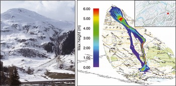
Fig. 1. Photograph of the Salezertobel avalanche (March 2008) within the test site Dorfberg and the corresponding RAMMS simulation. (Topographic map © swisstopo (DV033492.2).)
Vallée de la Sionne: open slope characteristics
In the Vallée de la Sionne the WSL Institute for Snow and Avalanche Research SLF has been operating a test site for large-scale snow avalanches since 1997 (Reference AmmannAmmann, 1999). Many avalanche events have been recorded using different techniques, such as airborne laser scanning, photogrammetry, videogrammetry, frequency-modulated continuous-wave (FMCW) radar and pressure sensors (Reference Sovilla, Schaer, Kern and BarteltSovilla and others, 2008). The slopes are less channeled than at the Dorfberg test site, and a long run-out zone is missing as large avalanches are stopped by the steep counterslope (Fig. 2). On 6 March 2006 two large mixed flowing/powder avalanches (Nos. 816 and 817) were triggered one after the other using explosives. Helicopter-based lidar data were acquired before and after the dry snow avalanche events to accurately document the release areas, release heights, mass balance and run-out distances (Reference Sovilla, McElwaine, Schaer and ValletSovilla and others, 2010).
Table 1. Common remote-sensing techniques to generate DEMs
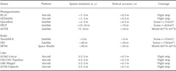
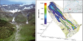
Fig. 2. Photograph of the Vallée de la Sionne test site and the RAMMS simulation of the large dry snow avalanche (6 March 2006) used for this study. (Topographic map © swisstopo (DV033492.2).)
Investigated digital elevation models
For this study we use high-resolution DEMs widespread in Switzerland (DTM-AV and DHM25) that are representative of DEM datasets available in countries with advanced geo-data coverage. Freely available DEMs, covering large parts of the Earth’s surface (ASTER, global DEM (GDEM) and SRTM) are also investigated. Such datasets may be used in countries where no high-resolution accurate DEM data are available. The ASTER and SRTM datasets were taken as delivered; no error corrections were performed. Figure 3 shows the shaded reliefs of the investigated DEMs, which have the following characteristics.
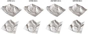
Fig. 3. Hillshades of the investigated DEM datasets (top: Dorfberg; bottom: Vallée de la Sionne,) showing the differing representation of terrain features with changing spatial resolution.
DTM 2m
This dataset has the best spatial resolution available for both test sites. For areas <2000ma.s.l., airborne lidar data with a spatial resolution of 2 m and a vertical accuracy of ∼0.5m are used (swisstopo, http://www.swisstopo.admin.ch/internet/swisstopo/de/home/products/height/domdtm-av.html). The elevation information for areas >2000ma.s.l. is derived from airborne optical scanner data (sensor ADS40, Leica HGeosystems, http://www.leica-geosystems.com/en/Leica-ADS80-Airborne-Digital-Sensor86846.htm) with similar spatial resolution and vertical accuracy of ∼1m in alpine terrain. This sensor has shown its usefulness for other applications in mountainous terrain, such as automated avalanche deposit detection (Reference Bühler, Hüni, Christen, Meister and KellenbergerBühler and others, 2009). Unlike the lidar technology, the optical scanner derives only DSMs. Even though there is only sparse elevated vegetation >2000ma.s.l., the ADS40 DSM has been smoothed using a low-pass filter to minimize the increased roughness caused by single trees, bushes and tussocks.
DHM 25m
The DHM 25m is derived from the 1 : 25 000 topographic map of Switzerland and was carefully checked for errors (swisstopo, unpublished information). It has a spatial resolution of 25 m and vertical accuracies of ∼2m within non-alpine terrain and of ∼3m within the Alps. Because of its long-time availability in Switzerland and its proven quality, the DHM 25m was used for the majority of studies in need of topographic information within Switzerland.
ASTER 30m
The ASTER sensor aboard the Terra satellite was launched in 1999. The visible/near-infrared subsystem acquires data at nadir (0˚ looking angle) and 27.7˚ backward-looking angle with a spatial resolution of 15m (Reference Yamaguchi, Kahle, Tsu, Kawakami and PnielYamaguchi and others, 1998). These data were used in 2009 to generate a GDEM covering the Earth’s surface between 83˚N and 83˚ S (ASTER GDEM Validation Team, http://www.ersdac.or.jp/GDEM/E/image/ASTERGDEMValidation Summary ReportVer1.pdf). The worldwide availability free of charge and the comparatively good spatial resolution make this DEM product very valuable for regions where no better national elevation models are available. Nevertheless, the ASTER DEM contains numerous errors in areas covered by clouds, in cast shadow or hidden by steep slopes. Therefore it must be checked carefully before using it for numerical simulations.
SRTM 90m
The SRTM was accomplished in February 2000 and generated a GDEM dataset covering 60˚ N–60˚ S with a spatial resolution of 1 arcsecond (∼90m). It was the first GDEM dataset freely available. The interferometric SAR (InSAR) technology is able to acquire data unaffected by cloud cover, which is particularly important in tropical areas (Reference FarrFarr and others, 2007). Due to the low backscatter signal over smooth surfaces (e.g. calm water bodies) and further constraints (e.g. radar shadow in mountainous terrain), the dataset is affected by numerous errors and must be checked carefully.
Methods
Numerical avalanche dynamics model, RAMMS
The following four depth-averaged equations are solved governing mass balance, momentum balance (Reference Pudasaini and HutterPudasaini and Hutter, 2007) and random kinetic energy production and decay (Reference Bartelt, Buser and PlatzerBartelt and others, 2006; Reference Buser and BarteltBuser and Bartelt, 2009):
The DEM is given as the function Z(X, Y) in a fixed Cartesian coordinate system X, Y, Z. The independent variables x and y denote the arc-length along the surface topography. The z-coordinate is perpendicular to the profile. Gravitational acceleration is given by the vector (gx , gy , gz ). The field variables of interest are the avalanche flow height, H(x, y, t ), the mean avalanche velocity, U(x, y, t)=(Ux (x, y, t ),Uy (x, y, t ))T, and the specific random kinetic energy density, R(x, y, t ). The magnitude and direction of the flow velocity are given by ∥U∥ = ![]() and the unit vector,
and the unit vector, ![]() respectively. We neglect centripetal accelerations (Reference Gray, M. and K.Gray and others, 1999), as we cannot define the exact running surface of the avalanche. High-curvature terrain features are often filled with snow, producing flat running surfaces of low curvature.
respectively. We neglect centripetal accelerations (Reference Gray, M. and K.Gray and others, 1999), as we cannot define the exact running surface of the avalanche. High-curvature terrain features are often filled with snow, producing flat running surfaces of low curvature.
The effective snow entrainment rate, Q̇(x, y, t ), is given by
and controlled by the dimensionless entrainment coefficient κ. The initial value h
s(x, y, 0) is given by the total height of the snow cover at position (x, y) and time t = 0 s. Because a naturally occurring snow cover exhibits a strong vertical structure, we allow bulk parameters, such as density and hardness, to vary with vertical position in the snow cover. We assume that the ith snow layer has height hi with constant snow density ![]() so h
s = ∑ hi .
so h
s = ∑ hi .
The right-hand side terms of the momentum equations, Equations (2) and (3), add up to an effective acceleration. The gravitational accelerations in the x- and y-directions are
The friction, S f = (S f, x , S f, y )T, is given by the extended Voellmy model which considers the effect of random kinetic energy, R, on frictional processes (Reference Bartelt and BuserBartelt and Buser, 2010):
Bartelt and Buser have found (Reference Bartelt, Buser and PlatzerBartelt and others, 2007)
indicating exponential relationships between the mean random kinetic energy and the frictional coefficients, μ and ξ:
when each constitutive process (Coulomb and turbulent) is considered individually. The frictional processes giving rise to μ(R) and ξ(R) depend on R, which is governed in Equation (4) by the production coefficient, α ∈ [0, 1], which defines the amount of granule scattering induced by shear, while the coefficient β > 0 can be considered the inverse
mean lifetime of the random kinetic energy. The constant, R 0, defines the exponential growth rate of friction as a function of the mean random kinetic energy density. The friction coefficients, μ 0 and ξ 0, are now constants that represent the static dry Coulomb and turbulent friction values
Measurements in Vallée de la Sionne show 4 ≤ R 0 ≤ 7kJm − 3 (Reference Bartelt and BuserBartelt and Buser, 2010), depending on the granulometric dimensions of the avalanches (Reference Bartelt and McArdellBartelt and McArdell, 2009). This provides μ values in good agreement with snow-chute experiments (Reference Platzer, Bartelt and KernPlatzer and others, 2007). Static dry Coulomb values can be deduced from deposition angles at the front of the avalanche, typically 0.40 ≤ μ 0 ≤ 0.55 (20–30 ˚ ), and ξ 0 (300 ≤ ξ 0 ≤ 800 ms − 2) is determined from avalanche tail velocities. The standard Voellmy–Salm model (Reference VoellmyVoellmy, 1955; Reference SalmSalm, 1993) can be recovered from the extended system by choosing α = 0. Due to the initial fluctuation energy being zero R(t = 0) = 0, this always ensures that R ≡ 0.
The governing differential equations are solved with second-order numerical schemes (Reference Christen, Kowalski and BarteltChristen and others, 2010b).
Simulation set-up
To investigate the influence of the DEM quality and resolution, we perform RAMMS calculations keeping all flow parameters constant, varying only the input DEM. For the Dorfberg test site we applied the standard Voellmy–Salm model (α = 0), generating the μ and ξ values for a large avalanche with a 10 year return period using a procedure documented by Reference Gruber and BarteltGruber and Bartelt (2007) and specified ‘no entrainment’, Q̇(x, y, t)=0.We simulated Vallée de la Sionne avalanches 816 and 817 using the extended Voellmy–Salm model with α = 0.1 and and β = 0.7 s − 1. These values were determined from velocity profile measurements (Reference Kern, Bartelt, Sovilla and BuserKern and others, 2009). We first simulated avalanche 816 on a 5 m grid, updating the DEM for avalanche 817. The results reported below are for the simulation of avalanche 817. The static friction coefficients, μ 0 and ξ 0, were taken to be μ 0 = 0.57 and ξ 0 = 550 ms − 2 (Reference Christen, Kowalski and BarteltChristen and others, 2010b). R 0 was set to 5 kJm3, in accordance with Reference Bartelt and BuserBartelt and Buser (2010). Avalanche 817 entrained 0.95 m of snow (κ = 1). For each case study, we use exactly the same release areas and release heights, calculation grid sizes, return periods, volume categories, snow densities, numerical calculation schemes and erosion parameters for the simulations within one test site. This approach ensures that the only source of differences between the simulations is the DEM.
Results and Discussion
Flow path
The simulation results at the Dorfberg test site show an evident influence of the DEM resolution on the flow path. While the results of the DTM 2m and the DHM 25m simulations are very similar, the southwestern sub-branches of the avalanches, which were observed in the field, disappear in the ASTER 30m and SRTM 90m simulations. Such changes in flow path can be observed within both test sites (Fig. 4 and 5).
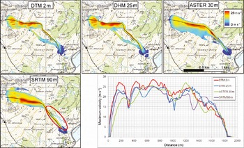
Fig. 4. Maximum velocity of the different simulations and comparison of the maximum velocity values within the Dorfberg test site. The black lines indicate the location of the profiles following the main flow path and indicate the line used to plot velocity vs distance. The flow path in the SRTM 90m simulation is shifted up to 100 m away from the gully (red circle). Note that profile paths had to be changed for the 30 and 90 m simulations due to divergence in the flow path. (Topographic map © swisstopo (DV033492.2).)
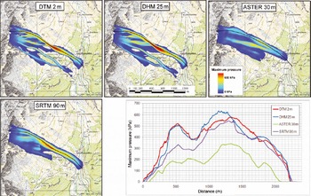
Fig. 5. Maximum pressure of the different simulations and comparison of the maximum pressure values within the Vallée de la Sionne test site. The black lines indicate the location of the profiles. Note that profile paths had to be changed for the 30 and 90 m simulations. (Topographic map © swisstopo (DV033492.2).)
At both test sites, the complex topography of the release and transition zones, containing many small channels and ridges, cannot be represented by the two coarsely resolved DEM datasets. Within the strongly channeled topography of Dorfberg, the avalanche path in the SRTM 90m simulation is shifted up to 100 m away from the gully (Fig. 4). The steep gully is not correctly represented and located by the coarse DEM resolution of 90 m. At Vallée de la Sionne, the flow path of the ASTER 30 m simulations is shifted up to 100m to the north and is stopped >300m too soon (Fig. 6). Clouds, cast shadows and steep slopes cause errors in the ASTER 30m DEM product (Fig. 7). The quality assessment file (QA), delivered with every ASTER GDEM tile, can help identify areas likely to be affected by errors (ASTER GDEM Validation Team, http://www.ersdac.or.jp/GDEM/E/image/ASTERGDEMValidation Summary ReportVer1.pdf). However, such anomalies and artifacts are hard to identify, and limit the usability of the ASTER 30m DEM as well as the SRTM 90 m.
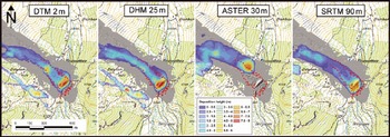
Fig. 6. Simulated avalanche deposits superimposed on helicopter-based lidar data (in gray) of the Vallée de la Sionne avalanche acquired in March 2006. The dotted red line indicates the reference deposition outline derived from the lidar data. The southwestern arm of the avalanche was not covered by the lidar data acquisition but was observed in the field. (Topographic map © swisstopo (DV033492.2).)
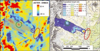
Fig. 7. Height deviations (left) of the ASTER 30 mm and the DHM 25mm DEM. The river bed is represented ∼25mm too high (red circle) and area to the northwest ∼30mm too low (blue circle) in the ASTER elevation model. Therefore the ASTER 30 mm RAMMS simulation (right image and outline superimposed in gray on the left image) deposits most of its material in the dump and stops before the avalanche reaches the valley bottom. Furthermore a false bump of ∼30mm in the middle of the slope (green circle) retains mass and leads to an incorrect deposition. (Topographic map © swisstopo (DV033492.2).)
Run-out distance and deposit
The comparison of the model results with measurements of observed reference avalanche events demonstrates the achieved accuracy of the DTM 2m and the DHM 25m simulations. Figure 8 shows that even small arms of the avalanche deposit are well represented. The break-out on the western part of the deposit can be explained by the levee, built up by the wet snow avalanche during its flow. This change in topography is not implementable without advance information. The shape of the deposit and the run-out distance are modeled significantly worse by the ASTER 30 m and SRTM 90m simulations on the open run-out slope at the Dorfberg test site. The material is sedimented in a circular deposit reaching further than the reference avalanche. The branches of the deposit are not modeled correctly.
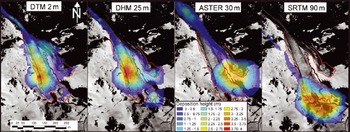
Fig. 8. Aerial imagery of the Salezertobel avalanche deposition with the simulation results superposed. The dotted red line indicates the reference deposition outline derived from aerial imagery.
The differences in run-out distance and deposit of the main avalanche branch are less obvious between the different simulations on the confined run-out zone at the Vallée de la Sionne test site. The main part of the material is deposited within the river bed at the bottom of the valley (Fig. 6). The sole exception is the ASTER 30 m simulation where the avalanche stops before it reaches the river bed. This change in run-out distance is caused by an incorrect representation of the river gully in the ASTER 30 m DEM. Figure 7 illustrates the deviations of the defective ASTER DEM, compared to the quality-checked DHM 25m DEM. The gully bottom is up to 30 m too high, damming the avalanche and stopping its flow. An incorrect dump just before the valley bottom leads to a precipitated deposition of the material. Such DEM anomalies and artifacts substantially limit the reliability of numerical avalanche simulations.
Flow velocities and impact pressure
Flow velocity and dynamic impact pressure are important parameters for hazard mapping, mitigationmeasure planning and safety assessment for buildings and infrastructure (Reference Margreth and AmmannMargreth and Ammann, 2004). Figure 5 illustrates the maximum pressure for the avalanche simulations at the Vallée de la Sionne test site. The profile graph along the main flow path of the simulations demonstrates the good agreement between the DTM 2m and DHM 25m simulations. The maximal pressure values and the shapes of the curves match well. The SRTM 90m simulation shows lower pressure values, especially within the upper part of the avalanche. The pressure values resulting from the ASTER 30 msimulation are only half of the DTM 2m and DHM 25m simulations. Due to errors in the DEM (see Fig. 7), a new avalanche branch, not existing within the other simulations, developed south of the main branch, dividing the available amount of snow and lowering the pressure. This example shows that such DEM errors can cause major failures in pressure simulations and could therefore lead to serious misclassifications in hazard maps.
Conclusions
Numerical avalanche simulations strongly depend on the underlying DEMs. Comparison of simulations using a DEM with a spatial resolution of 2 m (DTM 2 m) and one with a resolution of 25m (DHM 25 m) suggests that a spatial resolution of ∼25m is sufficient to accurately simulate large-scale dry and wet snow avalanches in three-dimensional mountain terrain. Simulated flow paths, run-out distances, deposits, velocities and impact pressures are in good agreement with the 2 m DEM simulations as well as with the reference observations in the field. This applies for the standard Voellmy–Salm model (used at the Dorfberg test site, α = 0, without entrainment) as well as for the extended random kinetic energy model (used at the Vallée de la Sionne test site, α ≠ 0, with entrainment).
The comparison of the simulation results demonstrates how coarse DEM resolution, as well as anomalies and artifacts of DEM data, can influence simulation results. Errors in the representation of terrain features such as gullies, ridges, hills or depressions lead to wrong and unrealistic flow paths (Fig. 4 and 5), run-out distances, deposits (Fig. 6 and 8), velocities (Fig. 4) and impact pressures (Fig. 5). If defective DEM data are used for hazard-mapping studies or safety assessments, serious mistakes are likely to occur. Based on these findings and further experience with RAMMS simulations, we advise caution when using DEM data with a spatial resolution worse than 30m, especially in complex terrain containing gullies and channels. Such features cannot be accurately represented by a coarsely resolved DEM. This can have a major impact on the simulated flow path, making the results unreliable and useless in many applications. However, previous avalanche events or snow accumulations by wind can significantly modify the terrain (Fig. 9). Therefore, we advise caution when using DEM datasets with a very high spatial resolution (better than 2 m) acquired in summer, because they may not represent the correct terrain for the simulated avalanche event. In our example problems, we did not vary the snow entrainment. But DEM characteristics could have an impact on entrainment rates. Further investigations will reveal the relationship between entrainment and DEM resolution.
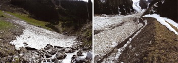
Fig. 9. Terrain modification caused by a previous avalanche event filling up a stream bed (left) and an artificial dam redirecting the avalanche path (right). Both images were acquired in the neighborhood of Davos, Switzerland.
Cost-free DEM datasets derived from satellite data, covering large parts of the Earth’s surface, are very valuable for regions not covered by high-resolution, high-quality national DEMs. This is still the case for the majority of regions in mountainous terrain. Available products (ASTER, GDEM and SRTM) have coarse spatial resolutions of 30–90m and, even more important, are affected by anomalies and artifacts. If such DEMs are used for modeling mass movements, such as snow avalanches or debris flows, they must be carefully checked for errors, using topographic maps, GPS measurements, photographs or DEM datasets from independent sources. The reliability of the simulation results will not be sufficient if no such checks can be performed, and they should not be used for critical applications such as hazard mapping or safety assessments.
For the simulation of medium- to small-scale avalanches, which cause the vast majority of casualties in Switzerland (Reference Harvey, Zweifel, Campbell, Conger and HaegeliHarvey and Zweifel, 2008) and threaten mountain roads and ski runs, the impact of DEM quality and resolution is even more critical. The flow path and run-out distance of such avalanches is to a greater extent dependent on small-scale terrain features. Future investigations will reveal the critical DEM quality and resolution for the simulation of such avalanches.


