

Nomenclature

Introduction
Observations on the Greenland Icecore Project (GRIP) and Greenland Ice Sheet Project Two (GISP2) ice cores have shown that polycrystalline ice develops a fabric which is induced by the strain undergone by ice as it descends from the surface to depth in the ice-sheet. At GRIP and GISP2 the fabric evolves from an isotropic fabric at the surface (crystals randomly oriented) to a vertical single-maximum fabric whose strength increases with depth.
Since the ice single crystal is strongly anisotropic, the polycrystalline response depends on the fabric strength and is also anisotropic. As shown by Reference Mangeney, Califano and CastelnauMangeney and others (1996), when polycrystalline anisotropy is taken into account in a flow model the general trend is an acceleration of flow compared to that of isotropic ice. In this flow model, anisotropy is given as an input and must be extrapolated between a few given data from a limited number of boreholes. However, in order to account for the anisotropy of ice more properly we have to consider the ice fabric as an unknown of the ice-sheet flow problem.
To solve this problem Reference Staroszczyk and MorlandStaroszczyk and Morland (2000) assume that the anisotropy of ice is entirely determined by the accumulated macroscopic deformation. In their model the stress is expressed in terms of the strain rate, of the accumulated strain and of three structure tensors, and all the mi-croprocesses taking place at the grain level are ignored. This model is very efficient, but does not provide results which can be compared to the fabrics observed in ice cores.
In the present paper, a complete solution, i.e. velocity and fabric fields, for the stationary flow of a two-dimensional ice-sheet is presented with an application to the flow of ice between GRIP and GISP2. This solution was obtained by incorporating a micro-macro model for the behaviour of anisotropic polycrystalline ice into a finite-element code for the flow simulation (for more details see Reference GagliardiniGagliardini, 1999; Reference Gagliardini, Meyssonnier, Hutter, Wang and BeerGagliardini and Meyssonnier, 1999a; Reference Staroszczyk and GagliardiniStaroszczyk and Gagliardini, 1999; Reference Gagliardini and MeyssonnierGagliardini and Meyssonnier, 1999b). Since the fabric in our model is calculated as an unknown of the flow problem the results can be compared to the fabrics measured in the GRIP and GISP2 cores.
Micro-Macro Model Assumptions
Notations
In the following, three Cartesian reference frame are used:
{R} is a fixed reference frame, whose plane (x1,x2) is the plane of the ice sheet flow, with x1 horizontal and x2 vertical upwards as shown in Figure 1.
{°R} is the material symmetry reference frame of an orthotropic polycrystal whose axes °xi coincide with the orthogonal privileged directions in the polycrystal. Furthermore it is assumed that the plane of symmetry (°Xl,°X2) of the polycrystal coincides with the plane (Xl,x2) of ice-sheet flow (i.e. °x3 = x3).
{gR} is a local reference frame associated with an individual grain, whose °x 3 axis coincides with the hexagonal symmetry axis of the grain (c axis).
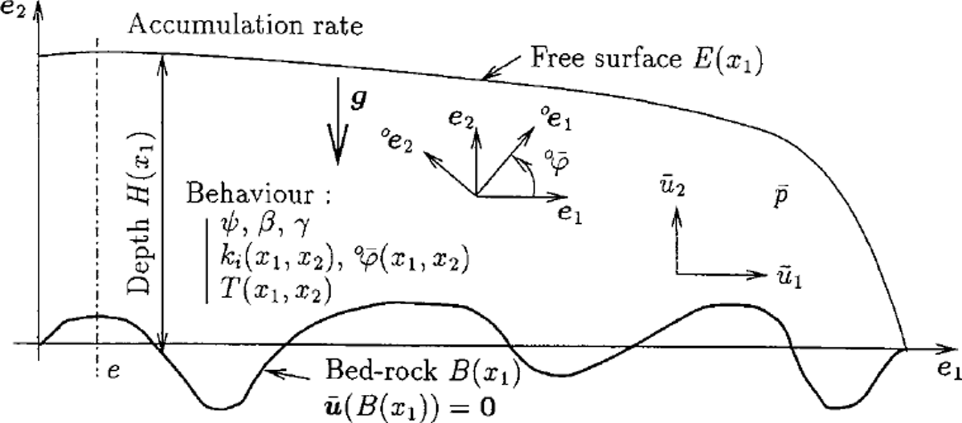
Fig. 1. Definition of the flow problem.
Macroscopic quantities associated to a polycrystal or to the ice-sheet are denoted by a super bar symbol. The superscripts "g"and o ’ are used to denote any non-scalar quantity expressed in the local reference frame {gR} and in the orthotropic symmetry reference frame {°R} respectively. Otherwise, if no superscript is applied, this quantity is expressed in the fixed reference frame {R}.
Grain behaviour
Following Reference Meyssonnier and PhilipMeyssonnier and Philip (1996) and Reference Gagliardini and MeyssonnierGagliardini and Meyssonnier (1999b) the ice crystal is assumed to behave as a linear transversely isotropic medium. The simplest relation between the strain-rate D and the deviatoric stress S is then expressed by
where M3 is the structure tensor defined by M3 = c ⊗ c and c is the grain c-axis unit vector (gc = (0, 0, 1) in the local reference frame). The parameter Ψ is the fluidity, inverse of viscosity, for shear parallel to the basal plane of the grain, and β is the ratio of the shear fluidity in the basal plane to that parallel to the basal plane. β is a measure of the grain anisotropy: when /3 = 0 the grain can deform only by basal glide, as assumed in many models (Reference LliboutryLliboutry, 1993; Reference Van der Veen and WhillansVan der Veen and Whillans, 1994; Reference Mangeney, Califano and HutterMangeney and others, 1997; Reference Godert and HutterGodert and Hutter, 1998), while 0 = 1 corresponds to an isotropic grain. Since the ice single crystal deforms mainly by shear parallel to its basal plane (Reference Duval, Ashby and AndermanDuval and others, 1983), the value of β should be significantly less than 1.
Orthotropic fabric
Following Reference Meyssonnier and PhilipMeyssonnier and Philip (1996), Reference Staroszczyk and GagliardiniStaroszczyk and Gagliardini (1999), Reference Gagliardini, Meyssonnier, Hutter, Wang and BeerGagliardini and Meyssonnier (1999a), the fabric of the ice polycrystal is described by a parameterized orientation-distribution function (ODF) which gives the relative density of grains whose c axes have the orientation (θ,φ) in the global reference frame {R}. This parameterized ODF which depends on four parameters is given by
The relation
which expresses the conservation of the total number of grains, is satisfied for any value of parameters ![]() and
and ![]() under the condition that
under the condition that ![]() . Relation (2) describes an orthotropic fabric with planes of symmetry (°x
1, °x
2), (°x
2, °x
3) and (°x
3, °x
1). In the following, the plane (°Xl, °x2) coincides with the plane (x1,x2) of the ice-sheet flow.
. Relation (2) describes an orthotropic fabric with planes of symmetry (°x
1, °x
2), (°x
2, °x
3) and (°x
3, °x
1). In the following, the plane (°Xl, °x2) coincides with the plane (x1,x2) of the ice-sheet flow.
Each parameter ![]() gives the strength of concentration of c axes in the direction °e
i
of the material frame {R°} at the material point × in the ice sheet (a small value of ki
corresponds to c axes gathered along direction °e
i
when
gives the strength of concentration of c axes in the direction °e
i
of the material frame {R°} at the material point × in the ice sheet (a small value of ki
corresponds to c axes gathered along direction °e
i
when ![]() the plane (°Xi,°Xj) is a plane of isotropy). The angle
the plane (°Xi,°Xj) is a plane of isotropy). The angle ![]() defines the rotation of {°R} with respect to the global reference frame {R} in the plane (Xl, x2) around the x3
axis (see Fig. 1).
defines the rotation of {°R} with respect to the global reference frame {R} in the plane (Xl, x2) around the x3
axis (see Fig. 1).
Behaviour of orthotropic ice
Under the assumption of a uniform state of stress in the polycrystal ![]() , the constitutive law corresponding to an orthotropic fabric (Equation (2)) is obtained by expressing the macroscopic strain rate as the weighted average of the grains strain-rate given by Equation (1). The resulting relation is
, the constitutive law corresponding to an orthotropic fabric (Equation (2)) is obtained by expressing the macroscopic strain rate as the weighted average of the grains strain-rate given by Equation (1). The resulting relation is
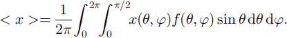
where (.)D denotes the deviatoric part of (.) and where the weighted average ≤. > of a quantity x(θ,φ) is defined as
The three structure tensors ![]() , in (4) are defined by the unit vectors °er of the material reference frame {°R} and the six response coefficients,
, in (4) are defined by the unit vectors °er of the material reference frame {°R} and the six response coefficients, ![]() are defined in terms of the grain rheological parameters ψ and β, and of the fabric parameters
are defined in terms of the grain rheological parameters ψ and β, and of the fabric parameters ![]() and
and ![]() (i.e.
(i.e. ![]() ) (see Reference Gagliardini, Meyssonnier, Hutter, Wang and BeerGagliardini and Meyssonnier (1999a) for these relations). For isotropic ice
) (see Reference Gagliardini, Meyssonnier, Hutter, Wang and BeerGagliardini and Meyssonnier (1999a) for these relations). For isotropic ice ![]() and the macroscopic orthotropic law (4) reduces to a linearly viscous law
and the macroscopic orthotropic law (4) reduces to a linearly viscous law ![]() where the fluidity
where the fluidity ![]() is related to the grain rheological parameters by (Reference Staroszczyk and GagliardiniStaroszczyk and Gagliardini, 1999; Reference Gagliardini and MeyssonnierGagliardini and Meyssonnier, 1999b)
is related to the grain rheological parameters by (Reference Staroszczyk and GagliardiniStaroszczyk and Gagliardini, 1999; Reference Gagliardini and MeyssonnierGagliardini and Meyssonnier, 1999b)
From (6) it follows that the ratio of the fluidity, ψ for shear parallel to the grain basal plane to the fluidity ![]() of isotropic ice reaches its maximum value of 2.5 when the grain behaviour is the most anisotropic (i.e. when /3 = 0). This value is lower than the experimental value of 10 obtained by Reference Pimienta, Duval and LipenkovPimienta and others (1987), therefore the influence of anisotropy on ice-sheet flow, as given by the present model, is under-estimated. The fluidity
of isotropic ice reaches its maximum value of 2.5 when the grain behaviour is the most anisotropic (i.e. when /3 = 0). This value is lower than the experimental value of 10 obtained by Reference Pimienta, Duval and LipenkovPimienta and others (1987), therefore the influence of anisotropy on ice-sheet flow, as given by the present model, is under-estimated. The fluidity ![]() (and also ψ according to Equation (6)) is related to temperature by the Arrhenius law
(and also ψ according to Equation (6)) is related to temperature by the Arrhenius law
where Q is the activation energy, R is the gas constant and T and T0 are temperatures in Kelvin.
Flow Problem
Equations and boundary conditions
The micro-macro model for the constitutive law of orthotropic ice was incorporated in a finite-element code in order to solve the gravity-driven, stationary, plane flow of an ice-sheet with fixed surface elevation and bedrock topography. Since the surface elevation is fixed, the accumulation rate must be considered as a variable determined by the solution of the flow problem. The flow problem to be solved and the notation used in this section are summarized in Figure 1.
The quasi-static stress-equilibrium equations corresponding to plane strain flow expressed in the fixed reference frame {R} are
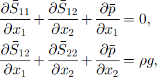
where ![]() is the isotropic pressure and pg is the density of ice times the acceleration of gravity. If ice density is assumed to be a constant then mass conservation reduces to the incompressibility equation
is the isotropic pressure and pg is the density of ice times the acceleration of gravity. If ice density is assumed to be a constant then mass conservation reduces to the incompressibility equation
where ![]() is the velocity component in direction ei.
is the velocity component in direction ei.
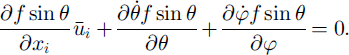
Since fabric evolution is supposed to be due solely to grain-lattice rotation (recrystallization is not accounted for), the steady-state condition ∂(fsin)/∂t = 0 at each point × in the ice sheet implies that the net flux of grains entering or leaving the interval (d0, dip) at point × (either by grain transport along the flow streamline or by change of orientation of the grain due to lattice rotation) is zero, that is
The grain rotation rates ![]() and
and ![]() in (10) are determined from the decomposition of the spin of each grain into a component due to its viscoplastic deformation (measured in the grain reference frame) and a component corresponding to the rotation of the basal planes (Reference Meyssonnier and PhilipMeyssonnier and Philip, 1996). According to Reference GagliardiniGagliardini (1999) and Reference Gagliardini and MeyssonnierGagliardini and Meyssonnier (1999b), under the assumption that the spin of the grain, W, expressed in the global reference frame {R} is equal to the macroscopic spin of the polycrystal
in (10) are determined from the decomposition of the spin of each grain into a component due to its viscoplastic deformation (measured in the grain reference frame) and a component corresponding to the rotation of the basal planes (Reference Meyssonnier and PhilipMeyssonnier and Philip, 1996). According to Reference GagliardiniGagliardini (1999) and Reference Gagliardini and MeyssonnierGagliardini and Meyssonnier (1999b), under the assumption that the spin of the grain, W, expressed in the global reference frame {R} is equal to the macroscopic spin of the polycrystal ![]() (Taylor-type assumption) the grain rotation-rates
(Taylor-type assumption) the grain rotation-rates ![]() and
and ![]() corresponding to plane flow can be expressed in terms of the deviatoric stress components
corresponding to plane flow can be expressed in terms of the deviatoric stress components ![]() ,
, ![]() and of the macroscopic spin
and of the macroscopic spin ![]() as
as

Equations (10) and (11) completely describe the evolution of the ice fabric in the particular case of a plane flow.
The stress on the ice-sheet free surface denoted by E =E(Xl)iS such that
where ns = (∂E/∂xu –1) is the outward unit normal to the surface and ![]() is the atmospheric pressure. Since the surface is assumed to be stationary, the velocity components
is the atmospheric pressure. Since the surface is assumed to be stationary, the velocity components ![]() and the vertical accumulation rate
and the vertical accumulation rate ![]() satisfy the kinematic condition
satisfy the kinematic condition
The ice deposited on the ice-sheet surface is assumed to be isotropic, therefore the fabric parameters ![]() have the fixed value
have the fixed value
No sliding is assumed at the ice-bedrock interface B = B(Xl), hence
and the vertical axis of symmetry of the (plane) ice sheet is assumed to be at x1 = e (see Fig. 1) which implies
Numerical methods
Using the orthotropic viscous law (4) for the behaviour of polycrystalline ice and with boundary conditions (12), (15), (16), the stress-equilibrium equation (8) and the incompressibility equation (9), are solved by the finite-element method. The isotropic pressure is used as a Lagrange multiplier in order to solve the incompressibility equation. The elements are six-node triangles with a linear interpolation of the pressure and a quadratic interpolation of the velocities and fabric parameters ![]() and
and ![]() .
.
The ODF parameters corresponding to stationary flow are obtained by solving the grain-conservation equation (10) along the streamlines computed from the finite-element solution for the velocities. The ODF parameters at each node M of the finite-element mesh are computed in two successive stages as follows:
the streamline passing through M is computed from M to the ice-sheet surface by solving the set of equations ![]() upstream procedure). During this phase S11, S22, S12 and the rotation rate
upstream procedure). During this phase S11, S22, S12 and the rotation rate ![]() are calculated at each fictitious time-step dt (corresponding to an increment of displacement along the streamline) by using the finite-element solution for the velocity and the constitutive law (4), then stored.
are calculated at each fictitious time-step dt (corresponding to an increment of displacement along the streamline) by using the finite-element solution for the velocity and the constitutive law (4), then stored.
the evolution of the ODF parameters along the streamline is calculated from the surface where ice is assumed to be isotropic (14). By assuming that the directions of the principal stresses do not change significantly during dt, the parameters ![]() are shown (see Reference GagliardiniGagliardini, 1999) to be the solution of
are shown (see Reference GagliardiniGagliardini, 1999) to be the solution of

where ![]() . During dt, the change of orientation of the material symmetry reference frame {°R}, i.e.
. During dt, the change of orientation of the material symmetry reference frame {°R}, i.e. ![]() is taken as the weighted average of the rotation
is taken as the weighted average of the rotation ![]() of the grains given by (11). These equations are solved using the Runge-Kutta method.
of the grains given by (11). These equations are solved using the Runge-Kutta method.
The velocity and fabric fields corresponding to stationary flow are calculated by solving iteratively the velocity problem for a given fabric field, then the fabric problem for a given velocity field, until convergence is achieved (i.e. when the norm of the relative deviation of each variable ![]() for two consecutive iterations is less than 1(T3).
for two consecutive iterations is less than 1(T3).
Application to the GRIP-GISP2 Flowline
Following Reference Schott, Waddington and RaymondSchott and others (1992) and Reference Hvidberg, Dahl-Jensen and WaddingtonHvidberg and others (1997), our model is applied to the flowline from GRIP to GISP2. The two boreholes GRIP (3238ma.s.L; Reference DansgaardDansgaard and others, 1993) and GISP2 (3215 ma.s.l.) are located in central Greenland, at 3 km and 27 km to the west of the actual summit of Greenland, respectively. Both boreholes have been drilled down to bedrock and their depths are 3029 m and 3053 m, respectively (Reference GowGow and others, 1997) (see Fig. 2). Many measurements have been made in this area and some of them are used as inputs to the model whereas others are used for model assessment.

Fig. 2. Surface and bedrock topographies, GRIP and GISP2 borehole locations and computed streamlines.
Model inputs
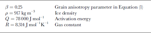
The numerical values assigned to the basic parameters are given in Table 1. The other assumptions are as follow:
The flow is plane strain and the two-dimensional flow domain presents a symmetry axis located at the actual summit of Greenland a t × 1 = ε = 3km. Its length is 184 km and it ends with a vertical free surface which should not influence flow in the vicinity of the two boreholes since it is located more than 50 ice thicknesses downstream from GISP2. The finite-element mesh contains 7351 nodes.
The flow is assumed to be stationary (in order to calculate a consistent field of fabrics) and the surface elevation is fixed according to field measurements (Reference Hodge, Wright, Bradley, Jacobel, Skou and VaughnHodge and others, 1990; see Fig. 2).
The bedrock topography conforms to that measured by Reference Hodge, Wright, Bradley, Jacobel, Skou and VaughnHodge and others (1990) taking into account the measurements of Reference Hempel and ThyssenHempel and Thyssen (1993) and Reference Jacobel and HodgeJacobel and Hodge (1995). For x1 φ- 4 0 km the bedrock is assumed to be flat (see Fig. 2).
The grain anisotropy parameter, /3, is given the value 13 = 0.25 and the fluidity, ψ is determined in terms of the fluidity of isotropic ice ![]() according to (6).
according to (6). ![]() is calculated by imposing an age of 14 450 years at 1753.4 m depth in the GRIP ice core (Reference JohnsenJohnsen and others, 1992).
is calculated by imposing an age of 14 450 years at 1753.4 m depth in the GRIP ice core (Reference JohnsenJohnsen and others, 1992).
The temperature field is derived from the profile measured in the GRIP borehole (Reference Gundestrup, Dahl-Jensen, Johnsen and RossiGundestrup and others, 1993) by assuming the temperature to be independent of the Xl coordinate and dependent on the reduced depth (ratio of depth to ice thickness). This assumption is justified since the temperature profiles at GRIP and GISP2 are very similar. The temperature increases from –31.7°C at the surface to –8.4°C at the bedrock.
The fabric corresponding to stationary state is calculated only in the domain –38 ≤ x1 ≤ 3 km and is extrapolated downstream (down to x1 = –181km) with the vertical profile of fabric obtained at x1 = –38 km.
Table 1. Value of the parameters used for finite-element computation
Results
As can be inferred from Equations (10) and (11), the fabric at a given point of the flow domain does not depend on the value of the fluidity of isotropic ice ![]() (nor on </>), which is consistent with the assumption of stationary flow. On the other hand
(nor on </>), which is consistent with the assumption of stationary flow. On the other hand ![]() acts as a scaling parameter for the velocities. By prescribing an age of 14 450 years at 1753.4 m depth for the ice of the GRIP core (Reference JohnsenJohnsen and others, 1992), the value of
acts as a scaling parameter for the velocities. By prescribing an age of 14 450 years at 1753.4 m depth for the ice of the GRIP core (Reference JohnsenJohnsen and others, 1992), the value of ![]() at –10˚C is found to bε
at –10˚C is found to bε ![]() . This value is lower than that inferred by Reference Lipenkov, Salamatin and DuvalLipenkov and others (1997) from bubble closure measurements
. This value is lower than that inferred by Reference Lipenkov, Salamatin and DuvalLipenkov and others (1997) from bubble closure measurements ![]() , but is still realistic.
, but is still realistic.
As shown in Figure 3, the computed horizontal velocities are larger than those measured by Reference WaddingtonWaddington and others (1995) and Reference Keller, Gundestrup, Dahl-Jensen, Tscherning, Forsberg and EkholmKeller and others (1995). Conversely the calculated accumulation rates are lower than those measured by Reference Dahl-Jensen, Johnsen, Hammer, Clausen, Jouzel and PeltierDahl-Jensen and others (1993) and Reference MeeseMeese and others (1994). Nevertheless, the horizontal velocities and accumulation rates obtained with the model are relatively close to the measurements.

Fig. 3. (a) Horizontal velocity ![]() and (b) accumulation rate
and (b) accumulation rate ![]() on the surface. The circles show the horizontal velocities measured by Reference WaddingtonWaddington and others (1995) and Reference Keller, Gundestrup, Dahl-Jensen, Tscherning, Forsberg and EkholmKeller and others (1995) and the accumulation rate from Reference Dahl-Jensen, Johnsen, Hammer, Clausen, Jouzel and PeltierDahl-Jensen and others (1993) and Reference MeeseMeese and others (1994).
on the surface. The circles show the horizontal velocities measured by Reference WaddingtonWaddington and others (1995) and Reference Keller, Gundestrup, Dahl-Jensen, Tscherning, Forsberg and EkholmKeller and others (1995) and the accumulation rate from Reference Dahl-Jensen, Johnsen, Hammer, Clausen, Jouzel and PeltierDahl-Jensen and others (1993) and Reference MeeseMeese and others (1994).
Figure 4 shows the ice-dating curves in GRIP and GISP2 calculated by the model compared to those measured by Reference JohnsenJohnsen and others (1992) and Reference MeeseMeese and others (1997). Since the value of ![]() was obtained by prescribing the age of the ice at 1753.4 m in the GRIP ice core the dated points are very well fitted by the computed curve from the surface down to this depth. For greater depths, and for both boreholes, the ages predicted by the model are younger than those measured. In the GISP2 borehole, the age is younger down to 2800 m, even though the no-sliding condition implies an infinite age at the bedrock contact. In Figure 4 a change in the curvature of the measured age vs depth curve at the Holocene-Wisconsin transition at 1650 m can be observed. This change is not reproduced by our model since the ice behaviour, the fabric and the temperature are evolving in a continuous manner with depth.
was obtained by prescribing the age of the ice at 1753.4 m in the GRIP ice core the dated points are very well fitted by the computed curve from the surface down to this depth. For greater depths, and for both boreholes, the ages predicted by the model are younger than those measured. In the GISP2 borehole, the age is younger down to 2800 m, even though the no-sliding condition implies an infinite age at the bedrock contact. In Figure 4 a change in the curvature of the measured age vs depth curve at the Holocene-Wisconsin transition at 1650 m can be observed. This change is not reproduced by our model since the ice behaviour, the fabric and the temperature are evolving in a continuous manner with depth.

Fig. 4. Evolution of the age of the ice vs depth in the GRIP (solid line) and GISP2 (dashed line) ice cores. Reference JohnsenJohnsen and others' (1992) dating in GRIP is represented by circles, Reference MeeseMeese and others' (1997) dating in GISP2 by triangles.
Fabric evolution in the GRIP ice core, represented by using Reference Thorsteinsson, Kipfstuhl and MillerThorsteinsson and others’ (1997) statistical parameter Ro, as well as the orientation ![]() of the material symmetry reference frame are shown in Figure 5. Ro characterizes the strength of the fabric and is defined as
of the material symmetry reference frame are shown in Figure 5. Ro characterizes the strength of the fabric and is defined as

Fig. 5. (a) Fabric strength parameter Ro in the GRIP ice core ( solidlme) and in the GISP2icecore (dashedline). Data from Reference Thorsteinsson, Kipfstuhl and MillerThorsteinsson and others (1997) in the GRIP ice core are shown by circles. The dotted line shows fabric evolution obtained with the model by using the ice strain-rate history derived from Dahl-of the Reference Dahl-Jensen, Johnsen, Hammer, Clausen, Jouzel and PeltierJensen and others’ (1993) model, (b) Orientation ![]() of the orthotropy reference frame a function of depth in the GRIP ice core (solid line). Data fromReference Thorsteinsson, Kipfstuhl and MillerThorsteinsson and others (1997) in the GRIP ice core are shown by the arrows.
of the orthotropy reference frame a function of depth in the GRIP ice core (solid line). Data fromReference Thorsteinsson, Kipfstuhl and MillerThorsteinsson and others (1997) in the GRIP ice core are shown by the arrows.
where c is the c axis unit vector expressed in the global reference frame {R}, ≤. > is the weighted average defined by Equation (5) and 11.11 is the norm of a vector. Ro is equal to 0 for a random fabric and takes the maximum value of 1 when all the crystals have the same orientation. Using Ro induces a loss of information on the fabric compared to the ODF description since the ODF (Equation (2)) contains three parameters to characterize the form and strength of the fabric. Nevertheless, since the strengths of measured fabric are given in terms of Ro (Reference Thorsteinsson, Kipfstuhl and MillerThorsteinsson and others, 1997) our results are presented under this form to allow comparison. As shown in Figure 5a the strengths Ro obtained with the model reproduce very well the measurements from 1000 m down to 2800 m. Above 1000 m the calculated values of Ro are lower than those measured, i.e. the model predicts a slower increase of the fabric. Below 2800 m fabrics induced by dynamic recrystallization are not reproduced by the model which does not take this mechanism into account. Figure 5b shows that the deviation from the vertical of the °x2 axis of the material symmetry reference frame is less than 2° in the GRIP ice core. According to Reference Thorsteinsson, Kipfstuhl and MillerThorsteinsson and others (1997) the average of the c axis directions does not deviate more than 10° from the axis of the ice core, and is usually within l°-6° from the core axis. Therefore the computed maximum value of 2° is compatible with the observations.
Discussion
Apart from its direct interest for ice-sheet-flow modelling, the comparison of the modelled fabrics to observation shows clearly the influence of flow conditions on fabric evolution. By using the Dansgaard-Johnsen flow model (Reference Dansgaard and JohnsenDansgaard and Johnsen, 1969) to provide a strain-rate history input to micro-macro models for anisotropic behaviour and fabric evolution, Reference Castelnau, Thorsteinsson, Kipfstuhl, Duval and CanovaCastelnau and others’ (1996) viscoplastic-self-consistent model as well as the present uniform-stress model (Reference Gagliardini and MeyssonnierGagliardini and Meyssonnier, 1999b) are found to predict a rate of fabric evolution greater than that observed below 650 m in the GRIP ice-core (see Fig. 5a). The Dansgaard-Johnsen one-dimensional flow model (Reference Dansgaard and JohnsenDansgaard and Johnsen, 1969) is based on the following assumptions: (a) the ice deforms under uniaxial compression with a constant vertical strain rate from the surface down to 1750 m (Reference Dahl-Jensen, Johnsen, Hammer, Clausen, Jouzel and PeltierDahl-Jensen and others, 1993), then the strain rate decreases linearly with depth down to zero on the bedrock; (b) the present accumulation rate of 0.23 mice eqv. a–1 is the mean accumulation rate during the Holocene; and (c) the surface and the bedrock are horizontal and with a constant ice thickness of 3028 m. In the present study the age of the ice was prescribed at a fixed depth and since the streamlines obtained with this two-dimensional flow model are not vertical the strain rates experienced by the ice are lower than those given by Reference Dansgaard and JohnsenDansgaard and Johnsen’s (1969) model. As a consequence, the accumulated strain at a given depth, and then the rate of fabric concentration vs depth, calculated by our model in the GRIP borehole are smaller than those given by Dansgaard andjohnsen’s (1969) model. Figure 6 shows the evolution of the strain rates ![]() and
and ![]() given by our flow model in the GRIP borehole (these are not the actual strain rates undergone by the ice in the ice core since the streamlines are not vertical).
given by our flow model in the GRIP borehole (these are not the actual strain rates undergone by the ice in the ice core since the streamlines are not vertical).
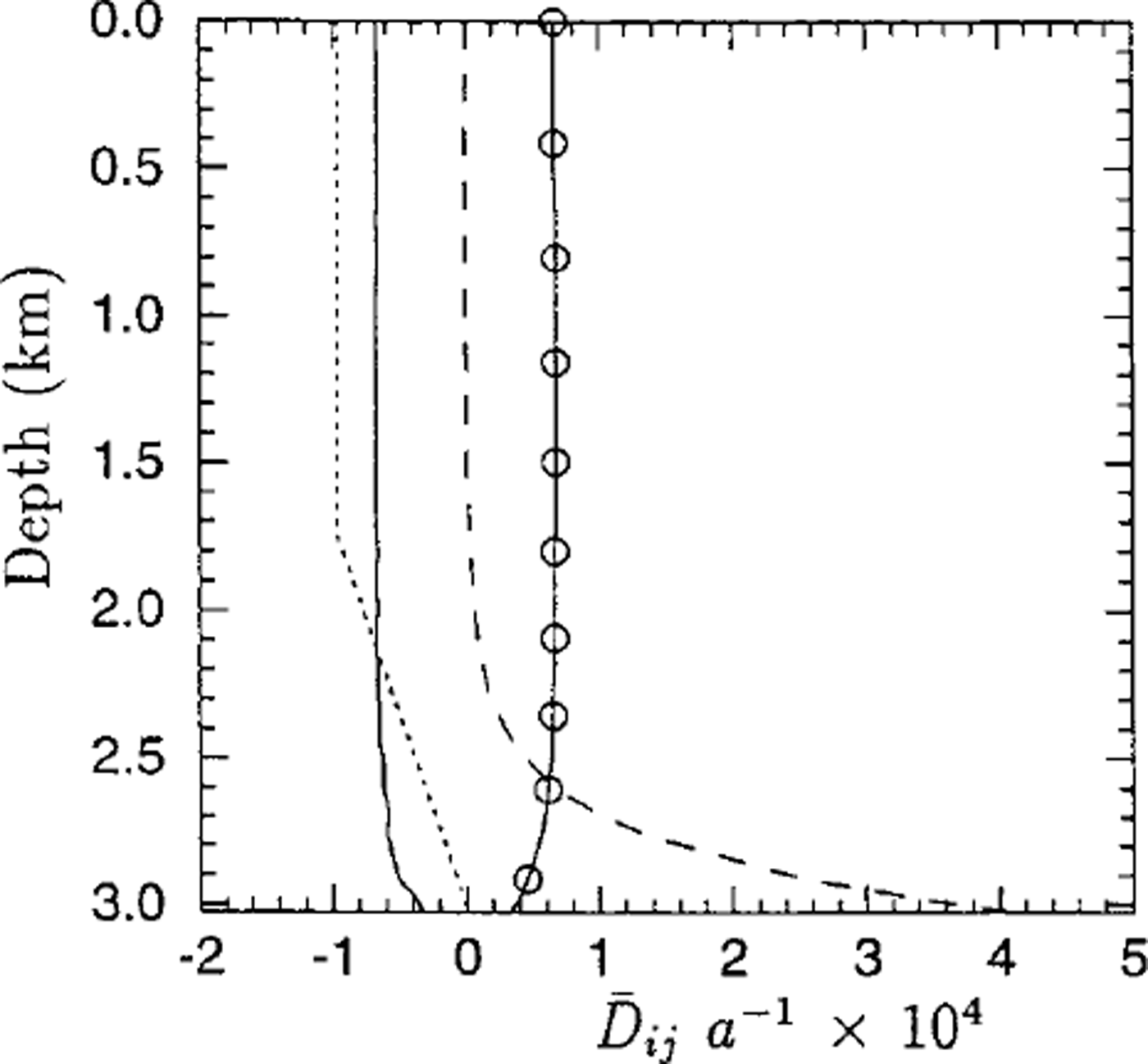
Fig. 6. Evolution of strain rates in the GRIP ice core as a function of depth: ![]() (solid line),
(solid line), ![]() (solid line and circle)and
(solid line and circle)and ![]() (dotted line). The dashed line shows the evolution of the strain rate
(dotted line). The dashed line shows the evolution of the strain rate ![]() assumed in the Reference Dahl-Jensen, Johnsen, Hammer, Clausen, Jouzel and PeltierDahl-Jensen and others’ (1993) model.
assumed in the Reference Dahl-Jensen, Johnsen, Hammer, Clausen, Jouzel and PeltierDahl-Jensen and others’ (1993) model.
As regards the assumed linear behaviour of polar ice, this assumption is justified at least for the upper part of ice sheets where the deviatoric stresses are very low (Reference Pimienta, Duval and LipenkovPimienta and others, 1987; Reference Lipenkov, Salamatin and DuvalLipenkov and others, 1997), however an extension of the model to non-linear behaviour is possible without theoretical difficulty when using the uniform-stress homogenization method (Reference LliboutryLliboutry, 1993).
Conclusion
A model for the linear mechanical behaviour of anisotropic polar ice and for the evolution of ice anisotropy has been coupled with a finite-element model to simulate the stationary flow of a two-dimensional ice sheet.
The basic ingredients of the micro-macro model are the description of the ice fabric by a continuous orientation distribution function (ODF) which gives the density of grains with a given c axis orientation, and Reuss’assumption of a uniform stress in the ice polycrystal which allows us to derive the mechanical properties of ice by homogenization, using the ODF as a weighting function. The ODF evolution is described by an equation of continuity, assuming that no recrystallization occurs.
The field of fabrics in the ice-sheet domain is described using a quadratic interpolation of the ODF parameters assigned to each node of the finite-element mesh. The finite-element solution of the flow problem for a given field of fabrics, obtained in terms of velocities, allows us to compute the trajectory of any material point of the flow domain as well as the strain history undergone by ice along this line. With the assumption of stationary flow, the knowledge of the strain-history along a streamline allows us to compute the corresponding fabrics. These two basic steps are repeated until convergence is achieved.
An application of the model to the flow between the GRIP and GISP2 drilling sites has been presented. The results of the model are in reasonable agreement with field data as regards the horizontal surface velocities, the magnitude of the accumulation rate and the strength of the fabrics measured along the GRIP core. They show that the flow conditions strongly influence fabric development.
Acknowledgements
This work was supported by the Commission of European Communities under contract ENV4-CT95-0125 "Fabric Development and Rheology of Polar Anisotropic Ice for Ice Sheet Flow Modelling". O Gagliardini was granted a BDI-scholarship by the Centre National de la Recherche Scientifique (Departement SPI): this financial support is gratefully acknowledged. The Laboratoire de Glaciologie et Geophysique de l’Environnement is associated with the Université joseph Fourier-Grenoble I.


