


1. Introduction
Sea ice plays an important role in polar climates by greatly modifying the radiative energy budget and mass processes. It is an important, sensitive and highly variable feature of the Earth’s surface. the amount of sea ice alters the amount of solar radiation absorbed by the ocean and modifies the heat, moisture and momentum transfer between the atmosphere and the ocean. In the ocean surrounding Antarctica, sea ice provides a continuous pathway for the reception and/or transmission of atmospheric and oceanic circulation anomalies. Those anomalies can in turn be communicated globally by the prevailing westerly atmospheric circulation and the Antarctic Circumpolar Current. Moreover, the annual cycle of ice growth and melt has a major impact on the ocean freshwater budget, while the behaviour of coastal polynyas affects the amount and location of deep and Bottom Water formation which plays a major role in global thermohaline circulation (Reference Drinkwater and LiuDrinkwater and Liu, 1997; Reference Comiso, Gordon and JeffriesComiso and Gordon, 1998). Therefore, sea ice has the potential to influence the world climate system over a wide range of timescales. It is thus important to understand the large-scale response of sea ice to changing patterns of atmospheric and oceanic circulation, anomalies of which are considered to be principal drivers of recently observed variability in the sea-ice extent and concentration (Reference HarangozoHarangozo, 1997; Reference Yuan and MartinsonYuan and Martinson, 2000; Reference Bitz, Fyfe and FlatoBitz and others, 2002; Reference Turner, Harangozo, Marshall, King and ColwellTurner and others, 2002; Reference Stammerjohn, Drinkwater, Smith and LiuStammerjohn and others, 2003).
Southern Ocean climate variability has been the subject of increasing interest during the last three decades. Antarctic sea-ice anomalies have been associated with atmospheric circulation variability in many data- and model-based studies. Data-based studies have shown relationships between sea ice and the large-scale circulation, but it is difficult to deduce from them whether sea ice affects circulation, which is also influenced by atmospheric processes (Reference Streten and PikeStreten and Pike, 1980; Reference Cavalieri and ParkinsonCavalieri and Parkinson, 1981; Reference CarletonCarleton, 1988, Reference Carleton1989; Harangozo, 1997; Reference Yuan and MartinsonYuan and Martinson, 2000). In contrast, studies based on general circulation models show a strong response to sea ice (Reference Mitchell and HillsMitchell and Hills, 1986; Reference Mitchell and SeniorMitchell and Senior, 1989; Reference Simmonds and BuddSimmonds and Budd, 1991; Reference Simmonds and WuSimmonds and Wu, 1993; Reference Walsh and ShuklaWalsh, 1993; Reference Bromwich, Chen and HinesBromwich and others, 1998; Reference Hudson and HewitsonHudson and Hewitson, 2001; Reference RaphaelRaphael, 2003). Nevertheless, the interpretation of the results should take into account the different ways in which the sea ice is included and/or whether the models consider the process of sea-ice formation and how the dynamics and thermodynamic processes involved are parameterized.
Reference Venegas and DrinkwaterVenegas and Drinkwater (2001) further proposed that anomalous atmospheric configurations generated sea-ice concentration anomalies of alternating sign in the southeastern Weddell Sea that were advected eastward out of the basin the following year by the gyre circulation. Otherwise, the variability in ice dynamics forces changes in northward ice extent, resulting in strong fluctuations in heat release from the ocean to the atmosphere in the region, which in turn caused changes in atmospheric pressure. This signal was obtained by means of multi-taper method singular-value decomposition (MTM-SVD; Reference Mann and ParkMann and Park, 1999), based on correlated variability among gridpoint time series. Reference Venegas, Drinkwater and ShafferVenegas and others (2001) also found a similar behaviour in the basins of the Ross, Amundsen and Bellingshausen Seas. on the other hand, Reference Yuan and MartinsonYuan and Martinson (2001) identified a dominant interannual variability in the sea-ice edge time series and surface air temperature, known as the Antarctic dipole (ADP). the ADP is characterized by an out-of-phase association between ice and temperature temporal anomalies in the central/eastern Pacific (centred in the northeastern Ross Gyre) and the Atlantic (central Weddell Gyre) sectors.
An atmospheric wave train of climate anomalies links equatorial and polar latitudes in the Pacific Ocean during El Niño Southern Oscillation (ENSO) events. According to Reference Houseago, McGregor, King and HarangozoHouseago and others (1998), there is a propagation of height and temperature anomalies from subtropical to high latitudes up to the event peak, with the anomalies persisting for ~1 year at subpolar latitudes. Reference HarangozoHarangozo (2000) showed that ENSO teleconnections indirectly influence west Antarctic Peninsula winter temperatures. Alterations in the local ice extent and above-normal pre-winter ice extent are necessary conditions for cold winters, but wintertime ice extent changes with ENSO-related meridional flow variations. Reference YuanYuan (2004) studied the composite analysis for five El Niño and five La Niña events to determine the relationship between Antarctic sea ice and the climatic variables, finding a positive feedback between the polar jet stream and stationary eddies in the atmosphere and within the air–sea-ice system that reinforces the anomalies, resulting in long-lasting ADP anomalies. the transmission of the ENSO signal to higher latitudes and evidence in the Antarctic meteorological and sea-ice records have been discussed by Reference TurnerTurner (2004) in his extensive literature review. He concluded that ‘we currently have a poor understanding of the transfer functions by which such signals arrive at the Antarctic from the tropical Pacific’ and that ENSO–sea-ice links have shown ‘the complex nature of the connections that are functions of the season and the sector of the Antarctic’.
Undoubtedly, increasing our knowledge of the relationship between variability in sea-ice conditions and atmospheric circulation around Antarctica is a high priority. According to Reference Yuan and MartinsonYuan and Martinson (2000), the Amundsen and Bellingshausen Seas and the Weddell Sea correspond to the sectors that record the greatest sea-ice temporal variability in the Southern Ocean. While the aforementioned studies have shown the close connection that exists between atmospheric circulation and sea-ice temporal anomalies in this area, they were based mostly on S-mode analysis of the covariability in time among the time series of gridpoints, using either empirical orthogonal functions (EOFs) or MTM-SVD. Both methods identify areas where statistically significant temporal sea-ice anomalies occur, without distinguishing whether they happen simultaneously (an important issue as the ice edge changes its position with seasons). Therefore, these methods provide the leading time-series patterns together with their corresponding centres of action in the spatial domain. Those areas cannot be compared with real fields; they just group the series in space according to their temporal variability. If the largest value at a centre of action exceeds a preselected threshold, it indicates that these series can be represented by the obtained temporal pattern. Reference Compagnucci and RichmaCompagnucci and Richman (2008) state that the S-mode approach provides standardized time series that correspond well only to those gridpoints with high absolute principal component loadings (centres of action) and that application of principal component analysis (PCA) in S-mode is appropriate if the goal of the analysis is to find spatial clusters of temporal series or teleconnections between the series and other variables.
The aim of this study is to analyse the spatial variability of sea ice around Antarctica and its relationship to the anomalous features of the main atmospheric circulation variables throughout the year (temporal clusters of fields of sea ice). We were looking for methods that could determine which atmospheric patterns accompany a given structure in sea-ice concentration. the acquisition of this kind of knowledge is impossible with EOFs/S-mode analysis because temporal studies do not give spatial structures. In this paper, we take a different approach by using T-mode PCA (Reference PreisendorferPreisendorfer, 1988; Reference JolliffeJolliffe, 2002), based on a correlation matrix between spatial fields, to obtain the leading spatial patterns of monthly sea-ice concentration anomalies (SICA). T-mode is the appropriate method if the goal of the analysis is to find spatial synoptic or flow patterns and when they happen in time (Reference Compagnucci and RichmaCompagnucci and Richman, 2008). In their discussion of S-mode and T-mode, Reference Compagnucci and RichmaCompagnucci and Richman (2008) show that these two approaches give different results which lead to dissimilar physical interpretations. They state that T-mode scores for correlation must be interpreted as standardized spatial patterns or ‘snapshots’, while the principal component loadings indicate at what time the patterns occur. In the T-mode, the set of the principal component scores can capture the input spatial patterns, and the loadings localize these patterns in time, which is consistent with the goals of spatial pattern classification, i.e. synoptic classification. Thus, the T-mode approach can be used to determine the spatial patterns and to provide a classification of the monthly SICA fields together with their intra- and interannual variability. With temporal clusters of this kind, it is easy to establish the relationships between SICA spatial structure and atmospheric circulation characteristics together with the frequency of occurrence for the different SICA/atmosphere coupled patterns. These are the patterns described and discussed in this paper.
2. Data and Method
2.1. Data
Monthly means of sea-ice concentration (the percentage of ocean covered by ice for a given region) over Antarctic seas and atmospheric circulation variables for the Southern Hemisphere are analysed for a period of nearly 31 years from January 1979 to September 2009. the data were obtained from Nimbus-7 scanning multichannel microwave radiometer (SMMR; 1979–87) and US Defense Meteorological Satellite Program (DMSP) Special Sensor Microwave/ Imager (SSM/I; 1987–2009) brightness temperature data. These data were processed by the NASA Goddard Space Flight Center using the NASA Team algorithm (Reference Cavalieri, Parkinson, Gloersen and ZwallyCavalieri and others, 2002) and provided by the US National Snow and Ice Data Center (NSIDC) mapped to a polar stereographic grid with a cell size of 25 km×25 km.
Atmospheric circulation relationships with the different SICA patterns were investigated using US National Centers for Environmental Prediction/US National Center for Atmospheric Research (NCEP/NCAR) reanalysis (Reference KalnayKalnay and others, 1996) monthly means of 850 hPa height and surface air temperature with a spatial resolution of 2.5˚ latitude ×2.5˚ longitude. Errors in NCEP/NCAR reanalysis at high latitudes of the Southern Hemisphere can be significant on a synoptic scale but become small in monthly mean values (Reference KistlerKistler and others, 2001). Monthly anomalies were computed prior to the PCA by removing the long-term 1979–2000 means and thus removing the annual cycle (this period was chosen to compare the results with those provided on the NSIDC webpage and with previous investigations).
2.2. Sea-ice concentration PCA
To isolate dominant SICA patterns, a T-mode (month-by-month) correlation matrix (Reference PreisendorferPreisendorfer, 1988; Reference JolliffeJolliffe, 2002; Reference Compagnucci and RichmaCompagnucci and Richman, 2008) was subjected to PCA. the statistical variables were the spatial SICA fields (number of variables n = 369 for the whole 31 year period), the domain was time and the statistical observations were the different gridpoints included in the area (number of observations M= 104 912). the resultant principal components (PCs) were Varimax-rotated iteratively to retain 2–20 components and calculate the congruence coefficient for each case to determine the goodness-of-match levels (Reference RichmanRichman, 1986). the results were principal component scores (PCS) that describe the leading modes of the SICA spatial variability and the associated time series called principal component loading (PCL); these represent the correlation between the PCS and each field of real monthly mean anomalies. Positive (negative) values of PCL were connected with the positive (negative) phase of the associated PCS. According to Reference Richman and GongRichman and Gong (1999), the absolute value of the loading designates a useful signal (hereafter called the loading ‘threshold’) for each PCS. the value of the threshold was obtained by Monte Carlo analysis, but these authors suggested that a value that ranges from 0.2 to 0.35, depending of the size of the sample and the variable analysed, will suffice to separate the PCS. Loading values that extend from zero to the threshold were ignored in the interpretation of the corresponding PCS because they could be due to noise or due to the fact that another PCS describes the behaviour there. Absolute values of loadings greater than the threshold increase the possibility of physical interpretation of the obtained PCS. In the present paper, the obtained threshold limit was ±0.3.
Owing to the fact that each PCL time series corresponded to the amplitude of the associated PCS for every monthly SICA, composites of SICA clustered for each PCS (as positive (negative) phase when loadings values were ≥0.3 (≤–0.3)) were shown instead of the PCS to facilitate the physical interpretation. Hereafter, the composites of SICA for each PCS were denominated by its numbered spatial pattern. As such, the first spatial pattern (PC1) in positive (negative) phase was used for the composites of the months that correspond to the first PCS with a value of PCL greater (less) than 0.3 (–0.3).
2.3. Climate analysis using PCL
The analysis of the interaction between SICA patterns and atmospheric circulation characteristics is performed through the composites for the months classified under each sea-ice concentration pattern of the atmospheric variable anomalies. For positive and negative phase of each pattern, an average of the variable under consideration (850 hPa and surface air temperature) is generated from all months that have a PCL value over the threshold (±0.3), in the same way as for the sea-ice patterns.
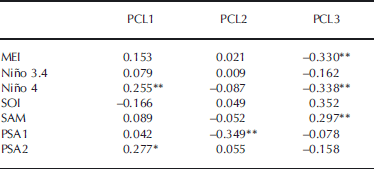
Linear correlations were used to test the PCL time-series trend and the occurrence of a SICA pattern in relation to ENSO and some other climate indices: the multivariate ENSO index (MEI), the Southern Oscillation Index (SOI), the East Central Tropical Pacific SST Index (5˚ N–5˚ S, 170˚ W–120˚W; Niño 3.4), the Central Tropical Pacific SST Index (5˚ N–5˚ S, 160˚ E–150˚W; Niño 4) and the Southern Annular Mode (SAM) obtained from http://www.esrl.noaa.-gov/psd/data/climateindices/, the first Pacific South America (PSA1) and the second Pacific South America (PSA2) indices defined by Reference Mo and HigginsMo and Higgins (1998). Table 1 shows the correlation values between the six PCLs and these indices. the PCL time series represent the amplitude of the PCS in each month, and the climatic signals are time series of specific numerical values. Therefore, the correlation coefficient could be interpreted as a rough estimate of the modulation in time of the previously named climatic signals over SICA patterns. the significance of the correlation coefficient was determined by Student’s t test.
Table 1. Correlation value between the six principal component loadings (PCLs) and the multivariate ENSO index (MEI), the Southern Oscillation Index (SOI), the East Central Tropical Pacific SST Index (5˚ N–5˚ S, 170˚ W–120˚W; Niño 3.4), the Central Tropical Pacific SST Index (5˚ N–5˚ S, 160˚ E–150˚W; Niño 4), the Southern Annular Mode (SAM), the first Pacific South America (PSA1) and the second Pacific South America (PSA2) indices. Student’s t test gives a significant correlation coefficient at the level of 90% or 95% of |r|≥0.23 (*) and |r|≥0.27 (**), respectively, with 50 degrees of freedom (considering an average persistence of 3 months in the SICA fields)
3. Spatial Behaviour
Sea-ice spatial patterns can be described in terms of the significant PCS. the first three PCS explained 38.07% of the total variance of the 124 summer–autumn months (January– April) for 1979–2009 analysed under the ±0.3 limits in the PCL time series. Figure 1 shows the PCL time series for PCL1, PCL2 and PCL3. It can be seen from Figure 1 that the PCLs showed differences in the temporal recurrence of each PCS. Table 2 shows the monthly classification of the sea-ice concentration anomalies for 1979–2009 obtained from PCL values (the number represents the PCS order: ‘+’ for positive phase and ‘–’ for the inverse). of all the months, 80.65% were classified under a PCS cluster. Only 16.93% of the months were clustered with a lower threshold (from –0.3 to –0.25 and from +0.3 to +0.25; in parentheses in Table 2) and a few of them (2.42%) corresponded to a winter pattern (WP in Table 2).

Fig. 1. Principal-component loading time series for (a) PCL1, (b) PCL2 and (c) PCL3. Period of analysis 1979–2009. the horizontal bold lines represent the threshold limit of ±0.3.
Table 2. Monthly classification of the sea-ice concentration anomalies for the period 1979–2009. the numbers indicate the order of the principal components (PCs) that classifies a month. the ‘+’ sign is associated with the positive phase of a PC, the ‘–’ sign with the negative phase. Numbers in parentheses indicate those months that obtained a lower than threshold PCL value. WP indicates a winter pattern

3.1. First principal summer–autumn pattern
During summer the sea-ice edge retreats southward towards its annual minimum. Furthermore the equator–Pole temperature gradient decreases and the atmospheric circulation is weaker than during winter. These relevant ocean– atmosphere–cryosphere characteristics are also present in the SICA patterns and the associated atmospheric variables. the leading monthly SICA pattern for summer and autumn explains 15.96% of the total variance. Table 2 shows that PC1 was present in 62 months of the period, indicating that 50% of the summer and autumn months had this pattern. the 26 months that correspond to the positive phase occur principally between 1981 and 1988, and the 36 months in negative phase are the principal pattern for the period 1991– 95 and the years 2003, 2008 and 2009 (Fig. 1a; Table 2). Figure 2 shows the sea-ice patterns in positive phase and in negative phase for PC1, PC2 and PC3. PC1 has a structure with two centres of equal sign located one over the Weddell Sea and the other over the Ross Sea and southwest Pacific Ocean and a centre of opposite sign over the Bellingshausen and Amundsen Seas (Fig. 2a: positive phase; Fig. 2b: negative phase).

Fig. 2. Sea-ice patterns of sea-ice concentration anomaly (%) for (a, c, e) the positive phase and (b, d, f) the negative phase for (a, b) PC1, (c, d) PC2 and (e, f) PC3. Negative values are in greyscale. Period of analysis 1979–2009.
The component loadings time series (PCL1) (Fig. 1a) clearly shows a change from positive to negative phase of the SICA pattern during 1989. This change has previously been associated with a modification in the shape and characteristics of the Weddell Gyre circulation at about 1990 (Reference Venegas and DrinkwaterVenegas and Drinkwater, 2001) and it can be related to the decadal variability in atmospheric circulation described by Reference Fogt and BromwichFogt and Bromwich (2006). None of the common waves longer than 1 year and described in the literature appear in the recurrence of this first pattern. Furthermore, Table 1 shows that PCL1 is not significantly correlated with the different indices. Only PSA2 (r = 0.277) and Niño 4 (r = 0.255) have a statistically significant correlation, showing a slight modulation of these two temporal signals over the occurrence of the PC1 spatial pattern.
The field of sea-ice concentration anomalies that appeared at the beginning of the sea-ice record (PC1 in positive phase; see Fig. 2a and 1a for the change in the pattern) presents a reduction in the sea-ice concentration over the Weddell Sea, the southwest Pacific Ocean and the Indian Ocean. on the other hand, the Amundsen and Bellingshausen Seas exhibit a positive value of SICA, probably because winter sea ice did not disappear completely along the coasts when this structure in sea-ice concentration was present. the opposite occurs during the months when the sea-ice anomalies are similar to this pattern in negative phase (Table 2; Fig. 2b). During the summer–autumn months when negative-phase PC1 occurs, sea ice over the Amundsen and Bellingshausen Seas is almost never present and most of the coastal areas of those seas remained ice-free, but the Weddell and Ross Seas registered an increase in average sea-ice concentration.
Figure 3 shows the resulting composite of the months classified under PC1 for 850 hPa height and surface air-temperature anomaly (SAT) fields for both phases. PC1 in positive-phase ice pattern is accompanied by climate trends associated with positive anomalies in the 850 hPa height field over the Antarctic continent and the adjacent seas (Fig. 3a) (a decrease in the intensity of the climatic low-pressure system over the Antarctic continent). the most intense positive anomaly is centred on the southwest Pacific Ocean southward of New Zealand. Negatives anomalies of 850 hPa height are located at middle latitudes around the Southern Ocean. These appear to be associated with an increase of cyclogenesis at mid-latitudes during the summers with less sea ice in the Weddell Sea. This structure is associated with positive anomalies of SATs in the regions with a decrease in sea-ice concentration (Weddell Sea and southwest Pacific Ocean) and with negative SAT anomalies over the Amundsen and Bellingshausen Seas (Fig. 3b). Taking into account the structure of height and temperature anomalies presented above, the increase (decrease) in sea-ice concentration over the positive (negative) areas (Fig. 2a) can be associated with the transport of sea ice northward (southward) by the wind and with the cold (warm) temperature advection.

Fig. 3. Composites of (a) 850 hPa height anomaly in gpm and (b) SAT anomalies in ˚C for PC1 in positive phase. (c, d) the same for PC1 in negative phase. Negative values are in greyscale, and contours are dashed lines. Period of analysis 1979–2009.
For the negative phase, the 850 hPa height anomaly field (Fig. 3c) is almost the opposite of the field described for PC1 in positive phase, but the negative anomalies over the Antarctic continent (including the negative maximum over the southwest Pacific Ocean) are not as intense as those of the positive phase (Fig. 3a). In fact, the positive anomalies are located at higher latitudes, for example the anomaly centred over the Amundsen Sea that extends along the Antarctic Peninsula into the northern Weddell Sea. This structure generates surface wind anomalies from the northeast over the Amundsen and Bellingshausen Seas (Fig. 3c) which together with the positive SAT anomalies (Fig. 3d) can be clearly associated with the decrease in sea-ice concentration over that region. In contrast, southerly and southwesterly surface winds together with the negative surface air-temperature anomalies help to maintain the positive anomaly of sea ice over the Weddell Sea.
3.2. Second spatial pattern
The second pattern (PC2) explains 11.19% of the total variance and corresponds to 36 months split into 14 months for the positive phase (Fig. 2c) and 22 months for the negative phase (Fig. 2d). This pattern is represented principally by two centres with opposite signs over the Weddell Sea forming a meridional dipole between the northern and southern Weddell Sea regions during both phases of this pattern (Fig. 2c and d). Even though the positive (negative) phase of this pattern presents a very extended region with positive (negative) SICA values in the external Weddell Sea, the opposite sea-ice conditions over the small area to the south are crucial, allowing (preventing) passage of ships to the Argentine station Belgrano II (77˚52’ S, 34˚37’ W) and the UK Halley research station (75˚35’ S, 26˚34’ W) in the southernmost region of the Weddell Sea. This pattern can be associated with the opening (closing) of the coastal polynyas there. the other characteristic that can be seen in this pattern is a region with the same sign of anomaly present in the northern region of the Weddell Sea over the Ross and Amundsen Seas. the Bellingshausen Sea shows the same sign of anomaly in both phases of PC2.
Figure 4 shows the resulting composite of the months classified under PC2 for 850 hPa height and SAT anomaly fields for both phases. the 850 hPa height anomaly fields in positive (negative) phase are characterized by positive (negative) height anomalies over the Antarctic continent with a very strong centre located over the Antarctic Peninsula. This pattern also comprises a belt of opposite-sign height anomalies between 70˚ S and 60˚ S in the positive phase and between 60˚ S and 30˚ S (not shown in the figure) for the negative phase (Fig. 4a and c). the positive phase can be associated with an increase of cyclogenesis over oceanic areas around Antarctica and southern South America. Conversely, the negative phase is associated with an intensification of the climatic pressure systems during the summer and autumn seasons when the spatial anomalies of sea ice resemble this pattern.

Fig. 4. Composites of (a) 850 hPa height anomaly in gpm and (b) SAT anomalies in ˚C for PC2 in positive phase. (c, d) the same for PC2 in negative phase. Negative values are in greyscale and contours are dashed lines. Period of analysis 1979–2009.
Temperature anomalies of both phases were almost opposite. the height anomaly fields for the positive (negative) phase gave wind anomalies from the south and southwest (from the north and northeast) westward of the Antarctic Peninsula over the area with negative (positive) SAT anomalies. These anomaly fields are concurrent with the positive (negative) SICA centre at the northern Weddell Sea (Fig. 4b and d) as well as over the Ross Sea (stronger in the positive phase). on the other hand, positive (negative) anomalies of surface temperature associated with the negative (positive) sea-ice anomalies occur in the southern Weddell Sea.
The PCL series (PCL2; Fig. 1b) shows no evidence of periodicity and no statistically significant trend from negative to positive values, although this pattern has been more prevalent since 1989 (Table 2; Fig. 1b). This pattern in negative phase was the one that characterized the sea-ice field during the break-up of the Larsen B ice shelf in 2002, leaving the northern region of the eastern Weddell Sea almost devoid of sea ice. Therefore, the dynamical process involved in the Larsen B break-up, analysed by Reference Scambos, Bohlander, Shuman and SkvarcaScambos and others (2004), could be associated with the occurrence of sea ice and atmospheric conditions described by PC2 in positive phase.
According to Table 1, PCL2 has an inverse statistically significant correlation with PSA1 (r = –0.349), which means that this mode of temporal variability modulates the temporal occurrence of PC2 spatial pattern in some way. Thus, PC2 can be influenced by the atmospheric pressure changes in the South Pacific sector. Apart from this, the different indices describing the ENSO signal are not correlated with PCL2, suggesting the absence of equatorial influence over this SICA spatial pattern.
3.3. Third spatial pattern
The third SICA pattern (PC3), which explains 10.92% of the total variance, is quite different from the bipolar structures presented in sections 3.1 and 3.2. the composites of the positive phase (12 months; Table 2) and the negative phase (13 months; Table 2) are characterized by anomalies of the same sign on both sides of the Antarctic Peninsula. These coincide with opposite-sign anomalies around the rest of the Antarctic, with the strongest anomaly centre located over the southwest Pacific Ocean and the Ross and Amundsen Seas (Fig. 2e and f).
Figure 5 shows the resulting composite of the months classified under PC3 for 850 hPa height and SAT anomaly fields for both phases. the atmospheric circulation associated with SICA in positive (negative) phase is characterized by negative (positive) 850 hPa height anomalies over Antarctica. the most intense is centred over the Bellingshausen and Amundsen Seas and extends to Drake Passage and the northwest Weddell Sea (Fig. 5a and c). Three opposite-sign centres are located over the southern region of the Atlantic, Pacific and Indian Oceans. Since the climatic low-pressure belt is located between 30˚ S and 60˚ S, the years that present a positive (negative) phase of SICA pattern can show a decrease (increase) in cyclone activity in this region. With this height structure, surface winds are from the north (south) over the eastern Weddell Sea flowing over an area with positive (negative) anomalies of surface temperature (Fig. 5b and d) in the positive (negative) phase. This temperature and wind structure helps to maintain the SICA present over the Weddell Sea. It is important to note that the positive (negative) temperature anomaly extends to the Bellingshausen Sea, where the sign of the SICA is the same as that over the Weddell Sea. on the other hand, extended negative (positive) anomalies of surface temperature occur elsewhere around Antarctica where surface winds are from the southern (northern) region, leading to positive (negative) SICA around Antarctica from the Indian Ocean to the Ross Sea.

Fig. 5. Composites of (a) 850 hPa height anomaly in gpm and (b) SAT anomalies in ˚C for PC3 in positive phase. (c, d) the same for PC3 in negative phase. Negative values are in greyscale and contours are dashed lines. Period of analysis 1979–2009.
Accordingly with the PCL time series (PCL3; Fig. 1c), the positive phase is present mainly in the latter part of the studied period (1996–2008), while the opposite phase appears during some summer and autumn seasons at the beginning of the period (1979–1992). the occurrence of this pattern seems to be dominated by a >30 year wave which cannot be represented due to the extension of the data series (only half of the wave can be seen in Fig. 1c). PCL3 shows a statistically significant trend from negative to positive phases (r = 0.24) (Fig. 1c). the 1990s trend of negative summer sea-ice anomalies over the Bellingshausen and Amundsen Seas that was previously observed for PC1 is reinforced by the occurrence of this summer and autumn pattern. Therefore, considering the occurrence of SICA second and third patterns (Table 2), the Amundsen and Bellingshausen Sea sectors exhibited summer and autumn seasons with greater than normal sea-ice concentration during the 1980s. At the same time, the Weddell Sea had a smaller than normal sea-ice concentration, combined with some years of higher than normal sea-ice concentration in its northern part and less than normal within the inner zone. the opposite occurred in the 1990s.
The 850 hPa height anomaly composites that correspond to PC3 (Fig. 5a and c) are similar to the EOF area clustered for the SAM temporal signal (Reference Visbeck and HallVisbeck and Hall, 2004). PCL3 and SAM series are significantly correlated (r = 0.297) for summer and autumn.
The composite fields of sea ice, low-level atmospheric circulation and temperature fields for PC3 in positive phase are similar to those corresponding to December–February (0 to +1 year) and March–May (+1 year) composites for La Niña events from 1984 to 2000 presented by Reference YuanYuan (2004). Although this pattern occurred during some La Niña summers, it also appeared during other summers under neutral conditions. Yuan’s (2004) inability to find the inverse condition could be due to the occurrence of the negative phase of this pattern only under neutral conditions of the ENSO which were not included in that paper (Table 2). In spite of this, the correlation values between the series and the MEI index (r = –0.330), Niño 4 (r = –0.338) and the SOI (r = 0.352) show a statistically significant correlation between PC3 and ENSO events. This fact can be associated with the occurrence of a La Niña event together with a positive phase of the SAM index (Reference Stammerjohn, Martinson, Smith, Yuan and RindStammerjohn and others, 2008) during 1999 when a positive phase of PC3 was also presented. This implies an association between cold events and positive values of SAM series with negative SICA over the Bellingshausen Sea.
4. Discussion and Conclusion
Using T-mode PCA, the main recurrent spatial structure of Antarctic SICA for summer and autumn months was obtained together with their temporal variability and associated atmospheric circulation patterns/anomalies. This is believed to be the first application of this method to obtain spatial patterns in SICA. Previous studies have analysed patterns of sea-ice temporal series anomalies using EOF methods (i.e. S-mode input matrix). Both types of approach provide different yet complementary results (Reference Compagnucci and RichmaCompagnucci and Richman, 2008). One provides temporal clusters of variable fields (T-mode), and the other spatial clusters of temporal series (S-mode).
The first three Varimax-rotated PCS, in positive and negative phases (six patterns), represent the most important features of the sea-ice spatial variability. the SICA patterns in positive (negative) phase were obtained from SICA composite for the months with component loadings over (below) the threshold of 0.3 (–0.3). It was possible to represent almost every summer and early-autumn month of the period 1979–2009 with one SICA pattern or a combination of two (Table 2) (temporal clusters). the relationship between sea-ice condition and atmospheric circulation was analysed using 850 hPa height and SAT anomaly composites for each SICA pattern.
During summer and autumn, the most frequent sea-ice concentration condition (represented by PC1) is a dipole anomaly structure between the eastern and western regions of Antarctica. the other frequent SICA pattern (PC2) exhibits a meridional dipole in the Weddell Sea, with opposing values in the inner vs the outer regions. the last sea-ice pattern (PC3) is characterized by strong anomalies of equal sign on both sides of the Antarctic Peninsula and opposite anomalies around the rest of the high-latitude Southern Ocean.
The results presented here confirm the strong relationship between sea-ice anomalies and atmospheric circulation noted in other studies of temporal data series of sea ice. During the warm months when the equator–Pole temperature gradient decreases, both the atmospheric circulation systems and the connection between the sea ice and the atmospheric conditions weaken.
Over the Amundsen and Bellingshausen Seas, greater than average sea-ice concentrations predominated during the 1980s followed by years with negative anomalies during the 1990s. This change is also reflected by the statistically significant positive trend in the component loadings time series (not shown in Fig. 1) and with higher incidence of PC1 in negative phase, PC2 in negative phase and PC3 in positive phase during the last part of the period under analysis. Over the Weddell Sea, this change in sea ice is less defined because the three summer and autumn patterns have a more complex spatial structure in that area.
It is difficult to determine what caused the sea-ice change that occurred during the warm seasons at the end of the 1980s and beginning of the 1990s. the Pacific Decadal Oscillation (PDO) equatorial signal, which is a long-lived El Niño-like pattern of Pacific climate variability, cannot be related directly to the change, because PDO presented a positive phase for the 1979–2000 warm seasons, with negative values only during the periods 1989–1991 and 1999–2000. In addition, large-scale Antarctic sea-ice temporal variability has been attributed to changes in SAM (e.g. Reference Fogt and BromwichHall and Visbeck, 2002; Reference Kwok and ComisoKwok and Comiso, 2002; Reference Lefebvre and GooseLefebvre and Goose, 2005). During the summer and autumn seasons of 1979–2009, it had a positive trend, with a change from negative to positive phase in 1993, compatible with the sea-ice signal in the Amundsen and Bellingshausen Seas. However, sea-ice anomalies precede the SAM temporal signal by ~3 years. on the other hand, Reference Burnett and NcNicollBurnett and McNicoll (2000) found that the Southern Hemisphere polar vortex contracted during the 1970s and 1980s, followed by a gradual expansion during the 1990s. the contraction is related primarily to geopotential height increases over the three mid-latitude oceans, while the expansion occurred as a function of geopotential height decreases throughout the polar region. Therefore, low-frequency variability in the circumpolar vortex area is in accordance with SICA change. This change in sea ice was also associated by Reference Venegas and DrinkwaterVenegas and Drinkwater (2001) with an alteration in the shape and characteristics of circulation in the Weddell Gyre at about 1990.
Our study has contributed to the understanding of the spatial variability of sea-ice concentration around Antarctica and has established the relationships between SICA spatial structure and atmospheric circulation characteristics, together with the occurrence of the different SICA/atmospheric couple patterns. Unfortunately, this method of spatial analysis did not allow us to establish whether sea-ice anomalies are the result or the cause of atmospheric anomalies. One can suppose that as sea-ice fields remain almost unchanged for longer periods than do atmospheric systems they may be the cause of some special structures in atmospheric circulation anomalies. Clearly, much work remains to be done to better understand the relationship between temporal and spatial patterns in large-scale Antarctic sea-ice anomalies noted in the current (spatial) and other studies (temporal) and the different modes of atmospheric circulation, which are interconnected in a complex fashion.
Acknowledgements
This study was supported by A0811 Proyecto bilateral: República Argentina (MINCYT) y el NRF de Sudáfrica, 2008/ 2010, PICT-2007-00438 AGENCIA-MINCYT, 2009/2011 and UBACYT X-016. We thank two anonymous reviewers for their thoughts on improving the manuscript and R. Massom, the Scientific Editor. We also thank NSIDC for providing the sea-ice data and M. Savoie who upgraded the data until 2009.


