


1. Introduction
As a fast-moving outlet glacier of the West Antarctic ice sheet (WAIS) that is characterized by low surface slope and grounding below sea level, Pine Island Glacier (PIG) has been recognized early on as a key factor in the stability of the WAIS (Fig. 1). While some authors expected that upward propagation of rapid retreat of PIG may cause the entire WAIS to surge (Reference HughesHughes, 1973) or turn the WAIS into an ice shelf (Reference WeertmanWeertman, 1974), other authors (Reference Crabtree and DoakeCrabtree and Doake, 1982; Reference Bentley, Giovinetto, Weller, Wilson and SeverinBentley and Giovinetto, 1991; Reference BentleyBentley, 1997) took a more conservative perspective.
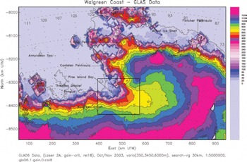
Fig. 1. Location of Pine Island Glacier on Walgreen Coast: 2003 GLAS data from submission L2A. GLAS release 18 data from GLA06 and GLA05 processed using gain criterion. DEM derived using kriging. Elevation in meters above WGS84. Universal Transverse Mercator (UTM) coordinates. Geographic coordinates overprinted on map. Box shows location of PIG study area. Modified after Reference Herzfeld, McBride, Zwally and DiMarzioHerzfeld and others (2008).
Reference Thomas, Sanderson and RoseThomas and others (1979) and Reference HughesHughes (1981) suggested that the northern part of the ice sheet could already be collapsing. From comparison of 1973 and 1975 Landsat imagery and 1966 aerial photographs, Reference SwithinbankSwithinbank (1988) derived 10km retreat or calving at PIG. In conclusion, PIG has been retreating for at least 40–50 years. Velocity in the 1990s was 2400 m a–1 (Reference Ferrigno, Williams, Rosanova, Lucchitta and SwithinbankFerrigno and others, 1998), increasing to 4200ma– 1 in 2009–11 (Reference Warner and RobertsWarner and Roberts, 2013). Retreat of the grounding line and increase in flow velocity has been observed from interferometric analysis of synthetic aperture radar (SAR) data (Reference RignotRignot, 1998, Reference Rignot2002; Reference Rignot, Vaughan, Schmeltz, Dupont and MacAyealRignot and others, 2002; Reference Schmeltz, Rignot and MacAyealSchmeltz and others, 2002; Reference Rabus and LangRabus and Lang, 2003), and changes in the ice from crevassing are visible in satellite imagery (Reference Ferrigno, Williams, Rosanova, Lucchitta and SwithinbankFerrigno and others, 1998; Reference BindschadlerBindschadler, 2002). Ice surface elevation mapping shows that the glacier is thinning by 3.125–12.5m a–1, depending on location, for the time interval 1995–2003 (Fig. 2a and b and 3a; Reference Herzfeld, McBride, Zwally and DiMarzioHerzfeld and others, 2008; cf. Reference Shepherd, Wingham, Mansley and CorrShepherd and others, 2001).
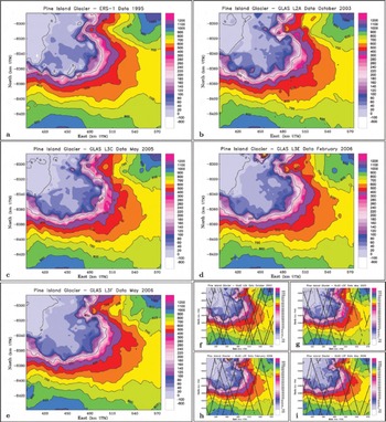
Fig. 2. Pine Island Glacier and the Pine Island Ice Shelf: elevation maps derived from ERS-1 and GLAS satellite altimeter data. (a) 1995 ERS-1 radar altimeter data. (b–e) GLAS (laser altimeter) data from ICESat: (b) 2003 October/November GLAS data from L2A, GLA06 data (release 18), from Reference Herzfeld, McBride, Zwally and DiMarzioHerzfeld and others (2008); (c) 2005 May GLAS data from L3C, GLA12 data (release 428), from Reference Herzfeld, McBride, Zwally and DiMarzioHerzfeld and others (2008); (d) 2006 February GLAS data from L3E, GLA12 data (release 428); and (e) 2006 May GLAS data from L3F, GLA12 data (release 428). (f–i) Same as (b–e) with GLAS ground track locations superimposed: (f) 2003 October/November GLAS data from L2A; (g) 2005 May GLAS data from L3C; (h) 2006 February GLAS data from L3E; (i) 2006 May GLAS data from L3F. UTM coordinates. Elevation in meters above WGS84. Maps based on DEMs calculated using ordinary kriging with search algorithms adapted to geophysical track-line patterns and a Gaussian variogram with nugget effect 350 m2 , total sill 3800 m2 and range 6km.
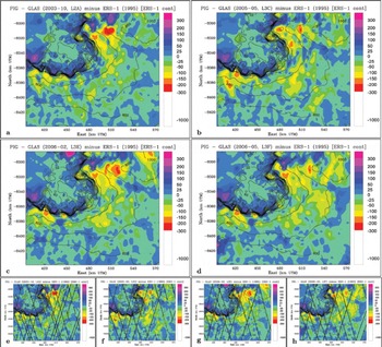
Fig. 3. PIG and PIIS elevation changes derived from ERS-1 and GLAS satellite altimeter data. (a) Elevation change over 8 years between 2003 (GLAS L2A, October/November 2003) and 1995 (ERS-1) (cf. Reference Herzfeld, McBride, Zwally and DiMarzioHerzfeld and others, 2008); (b) elevation change over 10 years between 2005 (GLAS L3C, May 2005) and 1995 (ERS-1); (c) elevation change over 1 1 years between 2006 (GLAS L3E, February 2006) and 1995 (ERS-1); and (d) elevation change over 1 1 years between 2006 (GLAS L3F, May 2006) and 1995 (ERS-1). (e–h) Same as (a–d) respectively, with satellite ground tracks from the GLAS component of the difference pair superimposed. 1995 ERS-1 contours of PIG and its ice shelf superimposed for reference. Note that the grounding line (hinge line) can be identified from the break in surface slope, as seen in the change in density of contours. UTM coordinates. Elevation change in meters.
Observation and analysis of changes in PIG are a central topic of current glaciological research. A summary to 2001 is given in Reference Vaughan, Bindschadler and AlleyVaughan and others (2001); a brief summary of recent research is given in Section 2.
As the future of PIG (and neighboring Thwaites Glacier) determines the future of the WAIS, it is important to understand the processes that cause and control the changes currently occurring in PIG. Significant data have been collected in field, aerial and satellite observation campaigns, and different authors favor different explanations for the observed change processes (see Section 2.3). Different processes lead to diverging estimates of the evolution of PIG and its ice shelf in the future and consequently different perspectives on sea-level change. Reference Joughin, Smith and HollandJoughin and others (2010) determine a model-derived maximum rate of sea-level rise from changes in PIG that is considerably smaller than previously thought, while Reference Park, Gourmelen, Shepherd, Kim, Vaughan and WinghamPark and others (2013) conclude that future contribution to sea-level rise may be higher than previously estimated, because the glacier–ocean system is not in a state of equilibrium.
This paper aims at attributing elevation changes and grounding line retreat in PIG to the physical processes that may cause them, for the time interval 1995–2003. The first objective towards this goal is to present spatio-temporal data and maps of elevation changes in PIG in recent years, derived from Geoscience Laser Altimeter System (GLAS) data collected during NASA’s Ice, Cloud and land Elevation Satellite (ICESat) mission of 2003–09 and comparison to radar altimeter data from the European Remote-sensing Satellite (ERS-1) collected in 1995. The second objective is to derive the evolution of elevation change in PIG in 2003–07 following accelerated retreat that has been observed for 1995–2003 compared to previous years (Reference Herzfeld, McBride, Zwally and DiMarzioHerzfeld and others, 2008; Reference Wingham, Wallis and ShepherdWingham and others, 2009).
In previous work, we reported that the spatial distribution of surface lowering in PIG in 1995–2003 suggests an attribution of changes to an internally forced process in the glacier (Reference Herzfeld, McBride, Zwally and DiMarzioHerzfeld and others, 2008; see Section 2.3). This interpretation is shared by Reference Rabus and LangRabus and Lang (2003). In recent years, retreat of PIG’s small ice shelf has been a dominant process and a topic of vigorous research, and much of the recent work associates changes in PIG entirely with processes in its ice shelf (Reference Payne and VieliPayne and Vieli, 2003; Reference Wingham, Wallis and ShepherdWingham and others, 2009; see Section 2). Reference VaughanVaughan and others (2012) observed large channels that formed under the Pine Island Ice Shelf (PIIS), caused by interaction of the bottom of the ice shelf with warming ocean water, and associated these with fracturing in the ice shelf.
The third objective of this paper is to discuss indications of processes that initiate from changes in the ice shelf vs processes that start internally in the glacier, based on the new observations and analysis. We formulate the hypothesis that both internal and external processes may control the changes in 1995–2007, whereas internally forced processes dominated in 1995–2003.
Prior to the data analysis, we give a summarized review of the state of the art of research on PIG related to the three objectives in Section 2. The literature review serves to substantiate the motivation for the work presented here.
2. State-of-the-Art Summary: Recent Changes in Pine Island Glacier and Pine Island Ice Shelf – Observations and Analyses
2.1. ICESat GLAS data analysis
Satellite altimeter data provide the best method for observing elevation changes in the large regions of the Earth’s ice sheets (Reference ZwallyZwally and others, 2002; Reference HerzfeldHerzfeld, 2004; Reference WinghamWingham and others, 2006, Reference Wingham, Wallis and Shepherd2009). Radar altimetry (e.g. ERS-1, ERS-2 and CryoSat) has the advantage of being able to penetrate clouds, which are frequent in the Arctic and Antarctic regions, whereas laser altimetry has the advantage of higher resolution but penetrates only thin clouds and is affected by thicker clouds and other atmospheric conditions. The GLAS system aboard ICESat has a footprint of 70 m and records point elevation every 173 m along-track (Reference ZwallyZwally and others, 2002; Reference Schutz, Zwally, Shuman, Hancock and DiMarzioSchutz and others, 2005). GLAS data provide the best available observations of ice-surface elevations through 2003-09. However, because of technical problems (loss of a laser, L1, early in the mission) the remaining lasers, L2 and L3, were only operated for two or three 33 day submissions per year to extend mission life. Track spacing depends on latitude (see Fig. 4 for the PIG region), nominal spacing is 22.93 km at 75° S for the 33 day missions, but actual track spacing may be two to three times that, because data losses are often caused by atmospheric conditions.
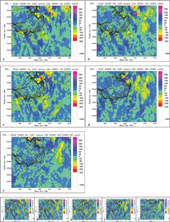
Fig. 4. PIG and PIIS elevation differences during GLAS observations: (a) over 3 years, February 2006 (L3E) – October 2003 (L2A); (b) over 3 years, May 2006 (L3F)–October 2003 (L2A); (c) over 2 years, May 2005 (L3C)–October 2003 (L2A); (d) over 1 year, May 2006 (L3F)–May 2005 (L3C); and (e) between seasons, May 2006 (L3F)–February 2006 (L3E). (f–j) Same as (a–e) respectively, with GLAS ground tracks from both missions superimposed (earlier mission tracks in red, later mission tracks in black). Surface-elevation contours of the earlier year/time superimposed for reference. Note that the grounding line (hinge line) can be identified from the break in surface slope, as seen in the change in density of contours. UTM coordinates. Elevation change in meters.
The figure of 22.93 km represents the spacing of ascending (or descending) tracks along the circle of 75° latitude, as well as the nominal width of the diamond-shaped gaps. Nominal spacing for the originally planned 91 day repeat orbit is one-third of the spacing of the 33 day repeat orbits, 7.64 km at 75° latitude. The tracks repeat only approximately, which makes it difficult to derive Δh/Δt without knowledge of cross-track slope.
Because of the above-mentioned difficulties in data distribution, the approach we adopt is to interpolate each submission dataset first, then form differences of digital elevation models (DEMs) (Reference Herzfeld, McBride, Zwally and DiMarzioHerzfeld and others, 2008). We derived elevation and elevation-change maps from ERS-1 data and early GLAS data collected near the beginning of NASA’s ICESat mission. Results showed that GLAS allowed elevation-change measurement from satellite altimetry with unprecedented accuracy and that PIG retreated at an increasing rate. The first two objectives of this paper are to extend this time series and to present a spatio-temporal analysis of the continued evolution of elevation changes in PIG.
Reference Pritchard, Arthern, Vaughan and EdwardsPritchard and others (2009) used ICESat release 28 GLAS data from February 2003 to November 2007 to derive maps of Greenland and Antarctica, which show extensive thinning on the margins of the ice sheets. They fitted planar surfaces to parallel tracks that are close in space (<300 m) and time (<2 years) and interpolated. The method sacrifices temporal resolution to gain spatial resolution of elevation change. Reference Pritchard, Ligtenberg, Fricker, Vaughan, Van den Broeke and PadmanPritchard and others (2012) concluded that the primary cause for Antarctic ice sheet loss is basal melting of the ice shelves, due to interaction with warmer ocean water. Lack of buttressing, resulting from ice-shelf loss, causes acceleration of the ice streams. Wind forcing could also play a role. Their paper presents thickness changes for all of the major Antarctic ice shelves and neighboring grounded ice for 2003–08, using a time series of repeat-track satellite laser altimetry. Ice-shelf thinning is reported as up to 6.8 m a – 1 in the Amundsen Sea sector. Maps in Reference Pritchard, Ligtenberg, Fricker, Vaughan, Van den Broeke and PadmanPritchard and others (2012) did not resolve the changes in PIG spatially or temporally. The first conclusion of the literature review is that a spatio-temporal analysis of elevation changes in PIG has not been presented previously. This motivates the derivation of a time series of maps from GLAS and ERS-1 for 1995–2007, which is the first objective.
2.2. Elevation and velocity changes from other datasets, and grounding line retreat
PIG is a focus area of glaciological research because changes predicted by authors 40 years ago are happening now. PIG has been losing elevation and increasing in velocity faster than predicted and at an accelerating pace. Reference Shepherd, Wingham, Mansley and CorrShepherd and others (2001) analyzed ERS-1 and ERS-2 radar altimetry and SAR interferometry to show that the grounded PIG thinned up to 1.6ma–1 between 1992 and 1999, affecting 150 km of the inland glacier, and concluded that the thinning cannot be explained by short-term variability in accumulation and must result from glacier dynamics. The map they presented is a collection of colored dots at crossover points, which makes spatial analysis difficult. Reference Herzfeld, McBride, Zwally and DiMarzioHerzfeld and others (2008) derived much higher thinning rates for the time interval 1995-2003 (3.125 m a–1 for 25 m difference, 6.25 ma–1 for 50m, and 12.5 ma–1 for 100m elevation difference, which depends on location), and surface lowering reached 50-100m in a ring segment 20-60 km from the 1995 hinge line (Fig. 3a; the hinge is identified by a break in surface gradient). Even with the lowest rate, thinning has increased considerably in 1995-2003 compared to 1992-99. It is not clear whether this process is continuing, which motivates the second objective of this paper.
Reference RignotRignot and others (2008) reported that ice-sheet loss increased 59% in 10 years in the Amundsen and Bellingshausen sea sectors of the Antarctic ice sheet, using 1992-2006 SAR interferometry along the margin of Antarctica to estimate total ice flux into the ocean.
Reference Wingham, Wallis and ShepherdWingham and others (2009) used ERS-2 and Envisat satellite radar altimeter data to examine spatial and temporal changes in the thinning rate of PIG in 1995-2006, applying a method of dual cycle crossovers. They provided maps of thinning rates in 1995 and 2006 and confirmed that thinning increased (e.g. to 6ma–1 in 2006 just above the grounding line). The main trunk of PIG and tributaries thin, but the slow-moving ice in the adjacent interior appears to thicken slightly. Reference Wingham, Wallis and ShepherdWingham and others (2009) assumed that the thinning is caused by ice drawdown propagating inland. If thinning continues to increase at the rate they derived, then the entire PIG trunk may become afloat in 100 years. Their analysis is based solely on widely spaced elevation-change points, which is a limitation when trying to identify spatial patterns.
Reference Herzfeld, McBride, Zwally and DiMarzioHerzfeld and others (2008) determined a grounding line retreat of ~20 km between 1995 and 2003 from ERS-1 and GLAS data analysis. The grounding line is determined as the break in slope between the ice shelf and glacier, as seen in the density of contours that are superimposed in elevation and elevation-difference maps in Reference Herzfeld, McBride, Zwally and DiMarzioHerzfeld and others (2008) and in this paper for different years. The 1999 grounding line, identified from differential SAR interferometry, is found in Reference Rignot, Mouginot and ScheuchlRignot and others (2011), and the 2009 grounding line is sketched in Reference Joughin, Smith and HollandJoughin and others (2010).
Reference Park, Gourmelen, Shepherd, Kim, Vaughan and WinghamPark and others (2013) investigated the position of the hinge line of PIG, based on 1992-2011 interferometric SAR data from ERS-1 and ERS-2 and found accelerated thinning (0.53±0.15 ma–1) at the terminus with comparable rates upstream, which is consistent with increased melting in a cavity below the ice shelf. They conclude that future contribution to sea-level rise may be higher than previously thought, because the glacier-ocean system is not in a state of equilibrium.
To determine the continuation of elevation change and grounding line retreat in PIG beyond 2003, we extend the time series to 2007. To study the evolution of these processes, we break the time series into annual and seasonal time steps, as much as GLAS data coverage allows (Sections 4 and 5).
2.3. Attribution of causes of the retreat
The changes in PIG may be caused by external forcing or internal forcing:
In an external-forcing scenario, break-up of part of the ice shelf in Pine Island Bay leads to loss of back-holding power that affects PIG. As a result, the glacier accelerates, first in the parts that are closest to the grounding line.
In an internal-forcing scenario, changes in the glacier or in its accumulation basin explain elevation and thickness changes. These may or may not affect the ice shelf. Changes in the glacier may have dynamical causes (acceleration) or climatic causes (changes in accumulation, or increase in surface melting). Changes in basal conditions may lead to changes in the glacier’s flow.
Despite the fact that the early debate on the future of change processes in the WAIS evolved around surging or slower glacial retreat, most more recent papers have attributed the observed changes to processes in the ice shelf. Reference Payne and VieliPayne and Vieli (2003) analyze how events in the ice shelf may lead to changes in the glacier and support an external-forcing hypothesis. Reference Rabus and LangRabus and Lang (2003) support an internal-forcing hypothesis and attribute observed break-off of large icebergs off the ice shelf to chance rather than an external mechanism.
Based on comparison of 1995 ERS-1 data and 2003 GLAS L2A data, Reference Herzfeld, McBride, Zwally and DiMarzioHerzfeld and others (2008) concluded that retreat of PIG is attributable to internal processes in the glacier. Comparison of a map based on 2003 GLAS data with a map derived from 1995 ERS-1 radar altimeter data clearly indicates mass loss in large parts of lower PIG and Pine Island basin, and far less change in the floating part of PIG tongue and the ice shelf in Pine Island Bay. The onlapping tongue of grounded ice seen on the PIIS, which was distinct in 1995 (Fig. 2a and b), has become shallower and narrower, while not shorter, in 2003. (The onlapping tongue is the tongue-shaped area above 40 m centered at 450000 E/ –8340000N in Figure 2a, identified by a break in slope seen in the density of contours; the tip of the arrow ‘Pine Island Bay’ in Figure 1 points at the same location.) The observations of elevation-change distribution indicate dynamic thinning, which is internally forced, as the most likely cause. One possible internal mechanism is a dynamic wave that propagates down-glacier. Acceleration in the glacier in 2003 was largest in the lower regions, where the observed thinning was greatest (Reference Herzfeld, McBride, Zwally and DiMarzioHerzfeld and others, 2008). The fact that surface lowering was largest, reaching 50–100 m, in a ring segment 20–60km from the 1995 hinge line (see Fig. 3a), while the total volume lost in the ice shelf was much smaller (maximally 25 m thinning over a smaller area), suggests an initiation of changes in the interior of the glacier. The internal dynamic changes might be a sign of a surge-type acceleration as expected by Reference HughesHughes (1973), or a different type of dynamic process.
According to Reference Rabus and LangRabus and Lang (2003), an acceleration with an amplitude of 12% of the PIG surface velocity extends 80 km up-glacier of the grounding line (in the determination of Reference Schmeltz, Rignot and MacAyealSchmeltz and others, 2002), which coincides with the area of surface lowering detected by our analysis (Reference Herzfeld, McBride, Zwally and DiMarzioHerzfeld and others, 2008). In the difference map (Fig. 3a), surface lowering extends at least to 700 m elevation.
In recent years, increasingly large changes have occurred in the PIIS. Reference VaughanVaughan and others (2012) observed basal melting under the PIIS, and related fracturing in the top of the ice shelf. PIG was grounded on a transverse ridge, but warm sea water has recently started to flow through a widening gap under the ice shelf, rapidly melting the thick ice of the newly formed upstream half of the ice shelf. Retreat of PIG was found to be unstable (Reference JenkinsJenkins and others, 2010). Data collected as part of NASA’s Operation IceBridge revealed the existence of a trough below the PIIS from the ice-shelf edge to the grounding line, which enables warm Circumpolar Deep Water to penetrate to the grounding line and lead to higher melt rates (Schodlock and others, 2012); a sensitivity study indicated that the cavity shape matters in this context. Reference ThomasThomas and others (2011) assumed that rapid thinning of the PIIS increases the likelihood of the ice shelf’s break-up and calculated the accelerating ice loss that may be expected to occur in this case, concluding that velocities in PIG may reach 10 km a–1.
Reference Payne, Vieli, Shepherd, Wingham and RignotPayne and others (2004, Reference Payne, Holland, Shepherd, Rutt, Jenkins and Joughin2007) attributed recent thinning in PIG to interaction of the PIIS with warm ocean water, and subsequent retreat of the PIIS. Reference Pritchard, Ligtenberg, Fricker, Vaughan, Van den Broeke and PadmanPritchard and others (2012) attributed ice-sheet loss in Antarctica generally to basal melting of the ice shelves. It is generally known that loss of an ice shelf will cause loss of buttressing and in consequence upward propagation of acceleration into glaciers that flow into this ice shelf, followed by mass transfer down-glacier. While this process is happening in the system of PIG and the PIIS, the question is whether the entire acceleration observed in PIG may be explained by mass loss from the ice shelf. O. Gagliardini (unpublished information) derived a new result from modeling, stating that changes in the PIG ice shelf cannot be the sole cause of the observed surface lowering and accelerations in the glacier.
Another different perspective on the possible sources of changes in PIG is given in studies of subglacial geophysics (Reference VaughanVaughan and others, 2006; Reference Scott, Gudmundsson, Smith, Bingham, Pritchard and VaughanScott and others, 2009). Reference Scott, Gudmundsson, Smith, Bingham, Pritchard and VaughanScott and others (2009) find that the increased rate of acceleration in PIG is strongly coupled to changes in gravitational driving stress. Using measurements of ice thickness, gravimetry, seismics and GPS-based surface elevation, Reference Smith, Bentley, Bingham and JordanSmith and others (2012) determine subglacial erosion beneath PIG at 0.6 ± 0.3 m a–1 at a location in the main trunk and conclude that subglacial erosion in a soft bed plays a significant role in ice dynamics. Subglacial topography of PIG is described in Reference VaughanVaughan and others (2006).
As this short literature review shows, there has not only been a wide range of data collection and analysis of the changes in PIG, there is also a wide range of interpretations of the changes in PIG. In summary, most authors favor a single process as an explanation for the retreat of PIG. The third objective of this paper is to relate the elevation changes that will be derived from the GLAS-data analysis to the geophysical processes that may have caused them.
3. Summary of Approach
To achieve the three objectives, (1) derivation of a spatiotemporal set of DEMs, elevation and elevation-change maps of PIG from GLAS data, (2) analysis of the evolution of elevation change in PIG and (3) attribution of observed changes to geophysical processes, the following approach is used. First, GLAS data from all ICESat submissions are corrected and processed until it can be determined which submissions yield sufficient coverage suitable for the purpose of this study. For each of the selected submissions a DEM is calculated, applying geostatistical estimation to derive values on a regular grid from the geophysical track line data that result from the satellite’s measurements along orbits. Next, elevation-change maps are derived. Sets of contours of a base topography (1995 for larger ranges of time, 2003 and later years for analysis of short-time changes) are superimposed to monitor changes in grounding-line position (more specifically, hinge-line position). Results of elevation and elevation-change mapping (objective 1) are presented in Section 4. This allows us to analyze evolution of changes in PIG and its ice shelf in more recent years (objective 2). Finally we investigate whether the elevation changes are indicative of forcing internal or external to PIG (objective 3).
4. IceSat Glas Data Analysis
4.1. GLAS instrumentation and ICESat mission parameters
In this subsection we provide a brief overview of ICESat GLAS instrumentation and data characteristics, as much as is needed to motivate the analysis methods. GLAS, the sole instrument aboard ICESat, is a next-generation space lidar. GLAS combines a precision surface lidar with a sensitive dual-wavelength cloud and aerosol lidar, emitting infrared and visible (green) laser pulses at 1064 nm and 532 nm wavelengths. The 1064 nm (infrared) laser channel is designed to measure surface altimetry and heights of dense clouds, and the 532 nm (green) lidar channel to measure the vertical distribution of clouds and aerosols. More precisely, the GLAS laser produces a 1064nm 40 Hz pulse for altimetry and lidar, and a Doppler crystal produces a 532 nm wavelength pulse, which yields a more sensitive determination of the vertical distribution of clouds and aerosols (Reference ZwallyZwally and others, 2002; Reference Schutz, Zwally, Shuman, Hancock and DiMarzioSchutz and others, 2005).
ICESat orbits at 600 km above the Earth’s surface. The footprint of GLAS is ~65 m in diameter, and the ‘spots’ illuminated on the Earth’s surface are separated by 172-173 m in the along-track direction. The echo pulse is accepted by a 1 m diameter telescope, directed to an analog detector, digitized by a 1 GHz sampler, along with a digitized record of the transmitted pulse. The digitized pulses constitute the waveform data, from which transmit and echo-receive time are determined. From the resultant two-way travel time, the range between the satellite and the Earth surface is calculated, and, using precision orbit determination based on GPS star tracking and post-processed improvement of the pointing accuracy of the laser, the elevation of a point on the surface is derived (Reference Schutz, Zwally, Shuman, Hancock and DiMarzioSchutz and others, 2005).
4.2. Processing of GLAS data to derive PIG DEMs
The ICESat mission was designed as a change-detection mission, so each submission was operated as a repeat-track mission. However, the spatial distribution of observations along ground tracks varies due to several factors. Clouds, aerosols and other atmospheric conditions cause frequent losses of altimeter data, especially in Arctic and Antarctic regions. Off-pointing maneuvers result in different track locations. The resultant ground-track locations are only close to repeat, but not exactly repeating, which complicates derivation of differences along-track without knowledge of local slopes. Therefore formation of differences directly from track data is not generally possible. Because of difficulties in the spatial data distribution, we calculate DEMs for each (sub)mission first and then form difference DEMs, on which the analysis of elevation changes is based. Finally spatial changes in the change patterns are analyzed.
Prior to geostatistical estimation of DEMs, the GLAS data are analyzed as follows (for a more detailed description of GLAS data processing, as well as ERS-1 data analysis, see Reference Herzfeld, McBride, Zwally and DiMarzioHerzfeld and others, 2008). GLAS data are recorded in 33 day submissions (L2A, L2B, etc.), and data products of different types are created by the NASA ICESat Project. Submissions are named after the lasers that were operated. Here we use products GLA06 (global elevation product), GLA05 (waveform product) and GLA12 (Antarctic and Greenland ice sheet elevation product). To match problems in recording L2A data, we derived a corrected dataset from a combination of data in GLA06 and GLA05 (a data point in GLA06 was rejected if the received gain value of the matching record in GLA05 exceeded 50). The submissions L2A (October/November 2003), L3C (May 2005), L3E (February 2006), L3F (May 2006) and L3I (October 2007) used in the following analysis have been selected, because the spatial coverage was good and because the energy levels in the lasers resulted in data of good quality. For these missions from L3C onward, we used GLA12 data (release 428). The release 428 data include a gain criterion that matches the one applied for L2A data in earlier work (Reference Herzfeld, McBride, Zwally and DiMarzioHerzfeld and others, 2008) to produce GLA12 data, with submission-specific gain-threshold values matching the decrease in laser power. The ICESat Project continues to reprocess GLAS data, implementing new corrections. However, elevation differences between releases are now very small compared to changes in PIG (centimeters or subcentimeters versus 25–150m elevation changes), hence reprocessing of the maps presented here is not necessary.
4.3. Geostatistical analysis
To calculate DEMs from GLAS data, the geostatistical interpolation/extrapolation method of ordinary kriging (OK) is applied, in the form adapted for analysis of geophysical trackline data, and, in particular, satellite altimeter data, described in detail in Reference HerzfeldHerzfeld (2004) (see also Reference HerzfeldHerzfeld, 1992; Reference Herzfeld, Lingle and LeeHerzfeld and others, 1993a, 1994, Reference Herzfeld, McBride, Zwally and DiMarzio2008, Reference Herzfeld, Wallin and Stachura2011). Kriging methods are methods of geostatistical estimation, commonly formulated in a probabilistic framework. For the ground-track patterns of GLAS data (Fig. 4) geostatistical estimation with OK performs an interpolation. The OK method proceeds by two steps: (1) variography and (2) interpolation. In step 1, an analysis of the spatial structure of the data is carried out, experimental variogram functions are calculated and then variogram models are derived, which in turn provide input values for step 2, the interpolation. The variogram model type and the variogram model parameters determine the spatial continuity or roughness of the resultant map. The estimation is based on a least-squares minimization with respect to an unbiasedness condition. For OK the unbiasedness condition is that the mathematical expectation is constant (in the neighborhood of an estimated point), which translates into the condition that the kriging weights sum up to one. For the analysis of PIG GLAS data, variograms are derived for different subareas: (1) Pine Island Glacier, tongue and ice shelf, (2) lower PIG, (3) middle PIG and (4) PIG basin. Maps are created using three variogram models and a number of kriging parameter combinations to select a single model to be used for all DEMs. A Gaussian variogram model with a nugget effect of 350 m2 , a sill parameter of 3450 m2 and a range of 6000m was used. The same variogram model is employed for all GLAS submission datasets and throughout the region to ensure that differences in elevations are only due to differences in the data and not to differences in the variogram model used. Studying the influence of the variogram on kriging results is not the objective of this paper but has been investigated in Reference Herzfeld, Eriksson and HolmlundHerzfeld and others (1993b).
The error is a combination of (1) the error in the data, which is affected by atmospheric conditions including cloud cover, ice-surface roughness, instrument- and laser-pointing errors and (2) errors associated with the interpolation method. Instrument- and laser-pointing errors can be neglected for GLAS data, compared to elevation changes for PIG. Elevation maps, and hence elevation-change maps, derived from satellite laser altimeter data are prone to errors in areas of high topographic relief. The color scheme in the elevation-change maps is chosen such that red/purple areas at both ends of the color scheme flag likely artifacts caused by topographic relief. It is known that altimeters lack accuracy over mountain ranges and ice-shelf edges (Reference Partington, Cudlip, McIntyre and King-HelePartington and others, 1987), while the accuracy of GLAS data has been determined as 2.1 cm over the interior of the Antarctic ice sheet, under clear-sky conditions and in areas of low slope (Reference ShumanShuman and others, 2006). For our study, this means that elevation changes over PIG and its ice shelf can be interpreted as geophysically caused, while accuracy over the adjacent Hudson Mountains (northeast corner of the map, northeast of the ice stream) is poor. Apparent elevation changes over Pine Island Bay may be due to changes in ocean altimetry or floating icebergs.
There are two possibilities for calculating the interpolation error of kriging: (1) the estimation standard deviation and (2) the numerical error. The estimation standard deviation (Reference HerzfeldHerzfeld, 1992) is a function of the variogram and hence increases with distance from the ground tracks, especially if a nearest-neighbor search is performed. The numerical error associated with propagating the data errors through the kriging equations depends on the noise levels and does not reflect the ground track patterns, as demonstrated in Reference Herzfeld, Lingle and LeeHerzfeld and others (1993a). However, the accuracy of a DEM and hence the quality of an elevation map can be improved by implementation of an alternative search routine.
The kriging software applied in the calculation of the DEMs used in the analysis in this paper includes a search algorithm specifically implemented for analysis of geophysical trackline data (part of the ‘advanced kriging’ algorithms of the author’s software). For grid nodes close to a ground track, the kriged elevation is based on points in a small neighborhood. If too few data points are found close to a grid node (as is typical for gaps between tracks), then a quadrant search is performed to ensure that an interpolation is carried out at the grid node controlled by observations taken in all directions that surround the grid node, rather than an extrapolation from data at the nearest track. This search algorithm serves to counteract the track pattern effect as much as possible. Close scrutiny of the elevation and elevation-difference maps that are overlain by track maps (Fig. 2b, 3b and 4b) shows that elevation features do not follow track patterns (Fig. 2b) and that local maxima and minima in elevation difference are found directly under the tracks as well as between them (Fig. 3b) for elevation changes over longer terms of 8–11 years. Short-termelevation change maps are somewhat influenced by track patterns (Fig. 4b), depending on track density, as absolute elevation changes are smaller and as regular tracks are missing due to signal absorptions in clouds.
In summary, by first calculating DEMs from altimeter data, elevation-change values can be derived for every point of a grid. Without gridding, elevation changes could only be derived at crossover points between ERS-1 tracks and GLAS tracks, or elevation-change analysis be limited to the time frame of a single satellite mission. A detailed analysis of the combined effects of satellite-altimeter-track spacing and kriging on the accuracy of resultant DEMs is carried out in Reference Herzfeld, Wallin and StachuraHerzfeld and others (2011) but is beyond the scope of this paper. The primary objective of this paper is the analysis of elevation changes for PIG over a long time frame which spans two satellite missions (1995–2007); this is geophysically meaningful after interpolation because the elevation changes are absolutely very large.
5. Elevation and Elevation-Change Maps and Results of Spatio-Temporal Analysis
Results of elevation mapping are presented in Figure 2.
Elevation change maps are calculated in two groups: (1) to study change over longer time intervals of 8, 10 and 11 years (Fig. 3), and (2) to study ice surface evolution over annual, biannual and seasonal intervals (Fig. 4).
First, we analyze and compare the change maps over 8, 10 and 11 years (Fig. 3): In the 2003 -1995 change map (Fig. 3a), the largest elevation changes on PIG are recorded around the 1995-400 m elevation contour up to the 1995-600 m elevation contour; surface lowering in this ring of elevation change is 50-100 m with local variations. As seen on the 2005-1995 change map (Fig. 3b), the area of largest elevation change remains upstream of the 1995-400 m contour, but elevation loss has increased another 50-100 m. Elevation loss since 1995 exceeds 150 m, and the region of large elevation loss has expanded further in the upstream direction by ~50 km. Areas of elevation loss exceeding 100 m in 10 years are now found above the 1995-600 m contour. The difference maps for the 11 year spans February 2006-1995 (Fig. 3c) and May 2006-1995 (Fig. 3d) show smaller regions of maximal elevation loss above 150 m (between the 1995-400 m and 600 m contours), but a further extension of the region of surface loss. In the map of elevation change over 10 years (Fig. 3b), the regions of elevation loss at the 1995-400-500 m contour and at the 1995-600m contour are interspersed with areas of small elevation gain (0-25 m), which form convex shapes approximately across-flow. These convexly shaped areas may indicate an alternation of areas of thinning and acceleration with areas of stagnation or small elevation gain in the along-flow direction of the glacier, which is interpreted as being caused by a dynamic process that initiates in the glacier. In the elevation-change maps that span 1 1 years, however, no more large areas of surface-height increase are found, and surface lowering appears to have spread up-glacier. Most areas are affected by 50–100m elevation loss. The latter observations suggest an upward propagation of mass loss in PIG, starting from the area where the internally caused change was first observed.
It has previously been suggested that all changes in PIG are driven by changes in its ice shelf. This analysis suggests that the situation is more complex, likely a combination of dynamic processes that initiate in the interior of the glacier and an upward propagation of effects in the ice shelf. A comparison of the maps of elevation loss over longer time spans (8–11 years) with maps of elevation change over short time spans (Fig. 4 and 5) suggests that there is no simple relationship between processes in the shelf and in the upper glacier.
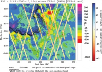
Fig. 5. PIG and PIIS elevation change over 8, 4 and 12 years. Map: elevation change over 8 years between 2003 (GLAS L2A) and 1995 (ERS-1). Along-track elevation differences between 2003 (GLAS L2A) and 2007 (L3I). ERS-1 contours of PIG and its ice shelf for reference. UTM coordinates.
In 1995, a tongue of grounded ice protruding into the ice shelf was prominent; this had grown much smaller and shallower by 2003. This is identified by the density of contours from 1995 and 2003 which are superimposed on the elevation-change maps. Mass loss in this tongue region continued from 2003 to 2006 (see the two maps of change over 3 years (Fig. 4a and b) and the map of change over 2 years, 2003–05 (Fig. 5c)) and indicates a grounding-line retreat. However, if loss in the ice shelf were the only driver of mass loss upstream, then the elevation loss further upstream would monotonously decrease from the shelf edge (grounding line) upstream. Instead, areas of largest surface lowering always appear around the 1995-400 m contour, and the area of second-largest surface lowering (1995-600m contour) is separated from the lower one by an area of near-stable surface elevation. In addition, the total mass loss from the PIIS is much smaller than the total mass loss from surface lowering in the glacier, as estimated from the area and elevation loss in the PIIS and in PIG; this observation provides an additional argument against explaining all changes in PIG only by changes in the PIIS. In conclusion, several processes contribute to the accelerations and mass loss throughout PIG.
The difference map L3F (May 2006)–L3C (May 2005) (Fig. 4d) suggests an anomaly of surface elevation increase in large regions of PIG. Notably, this is not a seasonal signal, as both L3F and L3C collected data in May, nor an artifact that may be associated with the ground-track pattern of ICESat. The difference map L3F (May 2006) – L3E (February 2006) (Fig. 4e) shows seasonal changes between February (late summer) and May (early winter) which affect large areas of PIG; values are generally in the elevation bins around zero, and increase dominates over PIG. Both maps L3F (May 2006)–L3C (May 2005) and L3F (May 2006)–L3E (February 2006) (Fig. 4e and f) suggest elevation loss northeast of PIG; however, this area is the most poorly constrained by observations in these difference maps.
In order to analyze changes in the elevation-change patterns throughout the observation time frame, we compare a long-term elevation-change map for 1995–2003 with elevation change evaluated along-track for 2003–07. This approach is chosen as a means to visualize differences of differences. Figure 5 shows elevation change along-track between 2003 (L2A) and 2007 (L3I) superimposed over the change map between 1995 and 2003. Largest elevation losses in the 4 years 2003–07 occurred just inland of the ice shelf (30–50m elevation loss), whereas the area of largest loss in the previous 8 years (1995–2003) is located farther upstream. This observation suggests the following conclusions: The initiation of acceleration earlier on occurred in the interior of the ice stream. In later years the locally largest elevation loss was driven by changes in the ice shelf, while surface lowering and likely acceleration continued to expand upstream in 2003–07 from the initial area of internal change. Elevation loss continued throughout the PIG region in 2003–07. Our findings suggest that more than one process causes the changes in PIG.
6. Summary and Conclusions
PIG is recognized as a key glacier whose continued retreat will determine the future of the WAIS. While a wide range of data has been collected in field, airborne and satellite campaigns, different researchers have favored different, single processes as the source of the observed changes. This motivates the primary goal of this paper: to attribute elevation changes and grounding line retreat in PIG to the physical processes that may cause them. There are two main processes: an internally caused acceleration in the glacier and an upward propagation of mass loss in the ice shelf. Towards this goal, three objectives are addressed: (1) derivation of a spatio-temporal set of DEMs, elevation and elevation-change maps of PIG from ICESat GLAS data, (2) analysis of the evolution of elevation change in PIG, and (3) attribution of observed changes to geophysical processes.
Time series of maps of surface elevation and elevation change in PIG and its ice shelf were calculated from ICESat GLAS data and ERS-1 radar altimeter data, using geostatistical analysis. Based on spatio-temporal analysis of elevation change between 1995 and 2007, we have discussed indications of processes that initiate from changes in the ice shelf vs processes that start internally in the glacier. Results of our analysis lead to the following conclusions: (1) Thinning rates continued to increase after 2003, regionally to >15 m a–1, with varying spatial patterns. (2) The initiation of acceleration earlier on has been in the interior of the ice stream (as already reported in Reference Herzfeld, McBride, Zwally and DiMarzioHerzfeld and others, 2008), while in later years largest elevation loss has been driven by changes in the ice shelf and upward propagation. (3) Surface lowering continued to spread upstream from the initial area of internal change in 2003–07. By 2006, the region of thinning had expanded up-glacier beyond the initial areas of surface lowering to 100 km above the hinge line. (4) In 2007, surface lowering was largest just up-glacier of the hinge line. (5) At least two processes have been causing the dynamically complex changes in PIG.
From analysis of ERS-1 and ICESat (GLAS) satellite altimeter data over the time frame 1995–2003, an internally forced process appeared to dominate the observed changes in PIG (Reference Herzfeld, McBride, Zwally and DiMarzioHerzfeld and others, 2008); however, from the extended analysis for the time frame 1995–2007 presented here, we conclude that at least two geophysical processes affect the PIG region.
Both internal glaciologic processes (initiating in the glacier itself) and external processes (initiating in the ice shelf or the ocean) contribute to changes in PIG. Observed external processes are warming of ocean water at the front of and below the PIIS, leading to interaction of warmer water with the ice shelf and retreat of the ice shelf (Reference VaughanVaughan and others, 2012). Likely internal processes are surge-type accelerations of the glacier, which may be related to changes in basal conditions. This result corresponds to the initial hypothesis of Reference HughesHughes (1973) that PIG, as a glacier with an extremely low gradient and one that is grounded below sea level, may accelerate as it starts to slide on increased amounts of basal water (see also Reference WeertmanWeertman, 1974). Inland propagation of this effect may lead to inland surge-type acceleration of the WAIS, according to Reference HughesHughes (1973). Attribution of the internally caused processes lies beyond the scope of this paper. The main contribution of the research presented here is to demonstrate that the spatial distribution of changes suggests at least two separate processes, one internal and one external to PIG, and two areas of change initiation, one in the ice shelf and one in the interior of PIG. The relative significance of the internally forced and the externally forced processes appears to change over time.
Acknowledgements
Thanks are due to John DiMarzio and David Hancock of the NASA Goddard Space Flight Center and Tim Urban of the University of Texas at Austin for discussions on data processing, to U.C.H.’s colleagues of the ICESat Science Team, the ICESat-2 ad hoc Science Team and the ICESat and ICESat-2 Projects for collaboration, to Patrick McBride, Danielle Lirette, Tyler Sears, Thomas Trantow, Alexander Weltman, Brian McDonald, all of University of Colorado Boulder, and to Almut Herzfeld Mayer for help with data processing and manuscript preparation, to editors Doug MacAyeal and Weili Wang and to anonymous reviewers whose help improved the manuscript. Support through NASA Cryospheric Sciences awards NNG04G062G (Pine Island Glacier), NNX09AO83G and NNX08AV90G to U.C.H. and through the University of Colorado Undergraduate Research Opportunity Program (UROP) is gratefully appreciated, the latter especially by B.W.


