1. Introduction
Greenland glaciers have been experiencing a growing mass deficit in the last two decades, half of which is caused by an increase in surface melt (Reference EttemaEttema and others, 2009; Reference Van den BroekeVan den Broeke and others, 2009) and half by an acceleration in glacier flow (Reference Rignot and KanagaratnamRignot and Kanagaratnam, 2006; Reference Rignot, Velicogna, Van den Broeke, Monaghan and LenaertsRignot and others, 2011). The acceleration was initiated in the glacier frontal regions and rapidly propagated upstream (Reference Joughin and Abdalati Wand FahnestockJoughin and others, 2004; Reference Thomas, Rignot, Kanagaratnam, Krabill and CasassaThomas and others, 2004). Several studies have examined the role of subglacial water in triggering the acceleration. The results suggest that this forcing is not sufficient to destabilize the glaciers and does not yield an increase in speed comparable in magnitude to observations (e.g. Reference Shepherd, Hubbard, Nienow, McMillan and JoughinShepherd and others, 2009).
Ocean warming has been hypothesized as an alternative cause of glacial destabilization (e.g. Reference Holland, Thomas, de Young, Ribergaard and LyberthHolland and others, 2008; Reference Howat, Smith, Joughin and ScambosHowat and others, 2008; Reference Hanna, Cappelen, Fettweis, Huybrechts, Luckman and RibergaardHanna and others, 2009; Reference MurrayMurray and others, 2010; Reference Rignot, Koppes and VelicognaRignot and others, 2010; Reference ChristoffersenChristoffersen and others, 2011). In Greenland, the vast majority of the ice discharged into the ocean is controlled by marine-terminating or tidewater glaciers, i.e. glaciers that terminate in the ocean, melt in contact with the ocean, and calve into icebergs. An increase in the temperature of the subsurface waters at the front of these glaciers would increase the subaqueous melt rates of their calving faces, cause retreat of the glacier fronts, and yield changes in force balance that could trigger speed-up. Floating ice tongues only exist north of 76˚N (Reference Rignot, Gogineni, Joughin and KrabillRignot and others, 2001). At low latitudes, Jakobshavn Isbræ (JKS; 698 N) was the only glacier that maintained a floating ice tongue until it disintegrated in 2002 (Reference Weidick, Mikkelsen, Mayer and PodlechWeidick and others, 2003). Reference Holland, Thomas, de Young, Ribergaard and LyberthHolland and others (2008) attributed its disintegration to the intrusion of warm Irminger waters into Disko Bay in the mid-1990s. A similar subtropical origin of oceanic heat was suggested by Reference Howat, Smith, Joughin and ScambosHowat and others (2008), Reference StraneoStraneo and others (2010) and Reference ChristoffersenChristoffersen and others (2011) for glaciers that accelerated in the east.
The Irminger Waters (IW) found around the margins of southern and western Greenland are named due to their advection through the Irminger Sea, the eastern lobe of the North Atlantic subpolar gyre (SPG). The variability of water mass properties of the IW is related to North Atlantic atmospheric forcing variability (Reference Myers, Kulan and RibergaardMyers and others, 2007). Variability of the North Atlantic atmospheric state is described in terms of the phase of the North Atlantic Oscillation (NAO). The NAO describes the large-scale westerly wind intensity and air–sea heat and buoyancy fluxes in the North Atlantic. During periods of sustained positive NAO index, intense westerly winds and large air–sea heat and buoyancy fluxes cause the SPG to expand which, in turn, reduces the amount of subtropical-origin waters entering the SPG from the North Atlantic Drift. A shift in NAO phase from high to low causes more subtropical-origin waters to enter the SPG and Greenland’s boundary current system. Moreover, since air–sea heat and buoyancy losses are positively correlated with the NAO, subtropical waters brought into the SPG are subject to less cooling during periods of negative NAO. Therefore, a switch from positive to negative NAO conditions is followed by a warming of IW in the SPG due to an increase in lateral ocean heat flux convergence and a decrease in air– sea heat loss (Reference Yashayaev and LoderYashayaev and Loder, 2009).
From the late 1980s to the early 1990s, the NAO was mainly in a positive phase, resulting in a cooler, fresher and laterally expansive SPG with comparatively colder and fresher IW in the SPG and the East/West Greenland Current (EGC/WGC). Following this period of sustained positive values, the NAO exhibited a dramatic reduction in the mid-1990s and remained mixed through the mid-2000s. The switch away from sustained positive NAO conditions led to a dramatic warming of the subtropical waters in the Irminger Sea. Soon thereafter, this warmer IW began to propagate around Greenland by EGC/WGC (Reference Myers, Kulan and RibergaardMyers and others, 2007). The warming of the subtropical-origin waters in the upper SPG and the IW component of the EGC/WGC has been observed with various in situ measurements (Reference Myers, Kulan and RibergaardMyers and others, 2007; Reference Holland, Thomas, de Young, Ribergaard and LyberthHolland and others, 2008; Reference Yashayaev and LoderYashayaev and Loder, 2009). Baffin Bay has far fewer contemporary in situ measurements relative to the SPG, but existing data suggest ongoing ocean warming in that region as well (Reference Laidre, Heide-Jørgensen, Ermold and SteeleLaidre and others, 2010).
Here we examine the propagation of anomalously warm subsurface temperature around Greenland from the mid-1990s using a high-resolution coupled ocean and sea-ice numerical simulation. The simulation is provided by the Estimating the Circulation and Climate of the Ocean, Phase II (ECCO2) project and it spans the 1992–2009 time period. We report changes in ocean temperature at several key regions around Greenland, compare the results with in situ observations, and summarize subsurface ocean temperature changes around the entire periphery of Greenland. Using the results of model simulations described in a companion paper (Reference Xu, Rignot, Menemenlis and KoppesXu and others, 2012), we then discuss the impact of these temperature changes on the subaqueous melt rates and their likely impact on glacier flow. We conclude on the relevance of the subsurface ocean for glacier stability in Greenland.
2. Model Configuration and Methodology
The results described herein are based on a regional configuration of the Massachusetts Institute of Technology general circulation model (MITgcm; Reference Marshall, Adcroft, Hill, Perelman and HeiseyMarshall and others, 1997). The domain of integration includes the entire Arctic Ocean and parts of the North Pacific and North Atlantic (see Reference Nguyen, Menemenlis and KwokNguyen and others, 2011, fig. 1). Model grid spacing is 4 km in the horizontal and ranges between 10 and 450 m over 50 levels in the vertical. The model employs the rescaled vertical coordinate z * of Reference Adcroft and CampinAdcroft and Campin (2004) and the partial-cell formulation of Reference Adcroft, Hill and MarshallAdcroft and others (1997). The ocean model is coupled to the dynamic and thermodynamic sea-ice model described by Reference Losch, Menemenlis, Campin and Heimbach Pand HillLosch and others (2010) and employs the salt plume parameterization of Reference Nguyen, Menemenlis and KwokNguyen and others (2009). Ocean and sea-ice model parameters are identical to the 18km optimized solution called A1 in Reference Nguyen, Menemenlis and KwokNguyen and others (2011). Ocean initial and lateral open boundary conditions of temperature and salinity are derived from the World Ocean Atlas 2005 (WOA05; Reference Boyer and LevitusBoyer and others, 2006) while velocities on the open boundaries are derived from the global, eddying ECCO2 state estimate of Reference MenemenlisMenemenlis and others (2008). Air–sea fluxes are calculated with the bulk formulae of Reference Large and YeagerLarge and Yeager (2008) and the Japanese 25 year reanalysis and the Japan Meteorological Agency Climate Data Assimilation System (JRA-25/JCDAS; Reference OnogiOnogi and others, 2007). Bathymetry is derived from the International Bathymetric Chart of the Arctic Ocean (IBCAO; Reference JakobssonJakobsson and others, 2008). A preliminary evaluation of the Arctic Ocean in the model is given by Reference Nguyen, Kwok and MenemenlisNguyen and others (in press).

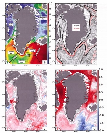
Fig. 1. Subsurface ocean temperature from the 4 km ECCO2 simulation overlain on IBCAO isobaths (Reference JakobssonJakobsson and others, 2008). (a) Averaged for the time period 1992–2009 at 250m depth (white areas are shallower than 250 m) with major locations discussed in the text. Sites are Kangerdlugssuaq Gletscher (KO and KS), southeast Greenland (SEO and SES), Nuuk (NO and NS), Jakobshavn Isbræ (JO and JS), Melville Bay (MO and MS), Petermann Gletscher (PO and PS) and 79 North glacier (79NO and 79NS). The AR7W, AR7E and eastern Baffin Bay evaluation boxes discussed in Figure 2 are dotted black lines. Diamonds (triangles) indicate the locations of on-shelf (off-shelf) three-dimensional boxes used to calculate the yearly-mean subsurface temperatures plotted in Figure 3. (b) Water velocity (cm s–1) at 250 m depth with location of major ocean currents: Irminger Current (IC), East Greenland Current (EGC), Labrador Current (LC) and West Greenland Current (WGC). (c, d) The 2001 (c) and 2009 (d) mean temperature anomalies at 250m from the model with respect to the 1992–2009 simulation period.
The realistic simulation of hydrographic variability and circulation dynamics in glacial fjords requires very high model horizontal resolution (<1 km), good bathymetric data, and, in some locations, representation of the effects of tidal forcing. Given the model resolution, the lack of a tidal submodel, and limited bathymetry knowledge, the model is analyzed near the mouths of the glacial fjords. Hydrographic changes at the fjord mouths may only be partially transmitted through the fjords to the glacier fronts. Most Greenland fjords are sill fjords (Reference BuchBuch, 2002; Table 1), i.e. warm subsurface waters have to overcome topographic barriers to penetrate the glacial fjords and reach the glacier fronts. Once at the ice fronts, these ocean waters participate in a vigorous convective circulation driven by subglacial water discharge at the glacier front, the buoyancy of fresh water at the front, and the pressure dependence of the melting point of sea water (Reference Motyka, Hunter, Echelmeyer and ConnorMotyka and others, 2003; Reference Xu, Rignot, Menemenlis and KoppesXu and others, 2012). When subglacial flow is low or absent, the forced convection is strongly reduced, and vigorous ice melting ceases as observed on Columbia Glacier, Alaska, USA (Walters and others, 1988).
Table 1. Characteristics of several major Greenland glacial fjords. NA: not available
3. Results
3.1. General trends
Figure 1a shows the simulated ocean temperature at 250 m depth, time-averaged for the entire 1992–2009 period. The warmest, saltiest waters are found to the east of the Reykjanes Ridge. These are subtropical-origin waters transported northward by the North Atlantic Current, with temperatures ≥8˚C at this depth. These waters are transported west by the Irminger Current (IC, Fig. 1b) towards southeast Greenland and north towards Svalbard and northeast Greenland by the Norwegian Atlantic and West Spitsburgen Currents. At the shelf along southeast Greenland they combine with the cold (1˚C), low-salinity shelf waters of the EGC coming from the Arctic and Nordic Seas (Reference Sutherland and PickartSutherland and Pickart, 2008) to form a two-component current with cold fresh waters above the shelf and warm salty waters along the slope. The EGC rounds the southern tip of Greenland at Cape Farewell to become the northward-flowing WGC, with subsurface ocean temperatures 2–3˚C lower than the IC, due to air–sea heat losses and lateral mixing. IW on the WGC is traceable in Figure 1 as the warm and fast-moving water flowing northward along the slope at 250 m. A portion of the WGC bifurcates west into the Labrador Sea and joins the Labrador Current (LC) to complete the western branch of the SPG (Fig. 1b). The non-bifurcating northward-flowing branch of the WGC passes through eastern Davis Strait into Baffin Bay (Reference BuchBuch, 2002). In northern Baffin Bay, the now significantly cooler IW on the WGC (1˚C) meets colder (≤0˚C), fresher southward-flowing Arctic currents from Nares Strait, and from Jones and Lancaster Sound. Together, these waters flow southward along Baffin Island in the Baffin Island Current (BIC) through western Davis Strait to the LC. In northeast Greenland, the subtropical-origin waters joining the EGC are much cooler (3.5–5˚C) than those waters joining farther south, a result of cooling during its northward transit.
The 4km ECCO2 solution reveals major changes in subsurface ocean temperature around Greenland between 1992 and 2009 (Fig. 1c and d). As the NAO ceased its sustained positive phase, IW in the SPG warmed and propagated along the EGC/WGC, yielding positive subsurface temperature anomalies in southeast, southwest and northwest Greenland. The warming around north and northeast Greenland took considerably longer, a result of the longer advective timescales associated with the propagation of subtropical-origin waters into the Greenland Sea and Arctic Ocean (Fig. 1c). During the second half of the simulation period the model indicates widespread warming in Baffin Bay and the Greenland Sea, and a cooling in the eastern Irminger Sea and southeast Greenland (Fig. 1d).
3.2. Comparison with in situ data
We compare the 4 km ECCO2 solution with in situ observations in the central Labrador Sea (within 150km of the AR7W line, in depths exceeding 3250 m), the western Irminger Sea (within 150km of the AR7E line, in depths exceeding 2500 m and west of 36˚ W) and in eastern Baffin Bay (71–74˚ N; east of 60˚W and in waters shallower than 550 m) (Fig. 2). Temperature data are drawn from conductivity-, temperature- and depth-measuring devices (CTDs), autonomous profiling floats and expendable bathythermographs compiled from Hydrobase 2 (R. Curry, unpublished information), the Global Temperature and Salinity Profile Program of the US National Oceanographic Data Center Operational Oceanography Group (2006) and the ICES (International Council for the Exploration of the Sea) Oceanographic Database and Services (2012).

Fig. 2. Comparison of subsurface temperature along the AR7W line (see dotted black box in Fig. 1a) in the central Labrador Sea from (a) in situ data and (b) ECCO2 4 km Arctic Ocean solution for the time period 1992–2009 minus an absolute offset of 0.4˚C. Similar plots in (c) and (d) along the AR7E line in the Irminger Sea (Fig. 1a), and (e) and (f) for the Eastern Baffin Bay evaluation box (Fig. 1a). Triangles in (a), (c) and (e) denote the availability of observations. Temperature is linearly interpolated in between except in (e) between 1991 and 1996 where the data gap is too large.
The 4 km ECCO2 simulation is initialized from the WOA05, a temperature and salinity atlas, which, by coincidence, includes several important observed features of the SPG in 1992 including a relatively cool and weakly stratified interior. Compared to observations in the Labrador and Irminger Seas between 1992 and 1996, the WOA05 has approximately +0.4˚C bias. This constant bias has been removed from the model results in Figures 2 and 3 in order to focus the discussion on temporal trends.

Fig. 3. Regional changes in subsurface ocean temperature from the 4 km ECCO2 simulation for the time period 1992–2009 minus an absolute offset of 0.4˚C. Left column is for off-shelf sites (triangles in Fig. 1a); right column is for on-shelf sites (diamonds in Fig. 1a). The size of the three-dimensional boxes used to calculate annual-mean subsurface temperatures is listed in Table 2. Left vertical axis indicates anomalies in subsurface temperature in reference to the average over the entire time period, between –1.5 and +1.5˚C, with vertical bars colored in red for positive anomalies and blue for negative anomalies. Right vertical axis in black is absolute subsurface temperature, with a scale that varies from site to site but not between on-shelf and off-shelf, except for KO and KS. Absolute temperature and anomaly calculations are insensitive to the particular trough or off-shelf location near each region (±0.2˚C) but are somewhat sensitive to the depth range (shelf) and offshore extent (off shelf) over which the calculation is made. Hence, both on- and off-shelf averaging volumes use the same depth range, chosen to be below the seasonal mixed layer and above on-shelf waters without significant temporal variability. The off-shelf volumes span the IW component of the boundary current where possible, or comparably sized regions off the shelf where not (PS).
Waters within the SPG have significantly warmed since the mid-1990s owing to a shift to generally milder wintertime atmospheric conditions. With reduced wintertime air–sea heat losses, net lateral advective heat flux convergence into the subpolar gyre has dominated over atmospheric heat loss. The model closely reproduces the magnitude and timing of the observed interior warming of the Labrador and Irminger Seas: about +1.0˚C in the upper 500m between 1992 and 2004 and +0.6˚C between 500 and 2000 m. In the Labrador Sea, temperatures in the upper 500 m cease their dramatic warming by 2004 and thereafter exhibit interannual variability consistent with known atmospheric variability (e.g. the cooling/deep-convection event of 2008; Reference VageVage and others, 2009).
We expect the simulated SPG warming to be limited for several reasons. Reference Lohmann, Drange and BentsenLohmann and others (2009) showed that the response of the SPG to a shift from NAO+ to NAO– conditions is sensitive to the amount of preconditioning by the atmosphere. The model initial conditions are identical to the WOA05 and are therefore not preconditioned by the NAO+ forcing, which began in the late 1980s. In addition, because the lateral ocean open boundaries are taken from WOA05, the waters feeding the SPG do not exhibit realistic interannual hydrographic variability. Finally, model–data differences include errors in the JRA-25/JCDAS surface boundary conditions and inaccuracies in the model subgrid-scale parameterizations.
Comprehensive model–data comparison is considerably more difficult for the eastern Baffin Bay region than for the SPG owing to the paucity of in situ observations over the simulation period, especially during the first 4 years when no measurements are available. Assuming that the ocean state in 1992 is similar to measurements taken in 1988 and 1990, the data indicate a warming of 1.0˚C between 100 and 300m between 1992 and 1999. At these depths, the model is initially ~1.0˚C cooler than observations, possibly an artifact of the sparse data used to generate the WOA05. However, the model warms to temperatures comparable to initial conditions by 1998 and then to contemporaneous observations by 1999–2000. A dip in 2005 temperatures is reproduced, as well as the subsequent 0.5˚C warming. Simulated temperatures in this region for the 2000s are in broad agreement with narwhal-based observations reported by Reference Laidre, Heide-Jørgensen, Ermold and SteeleLaidre and others (2010) who found maximum wintertime temperatures up to 3.4˚C at 350 m in the same region.
In terms of total temperature change, the model exhibits an extra degree of warming in the eastern Baffin Bay region compared with that observed. Without additional experiments it is impossible to determine how much of the warming is due to a realistic model response to the specified atmospheric forcing, as opposed to the model evolving away from imperfect initial conditions or to systematic model errors. It also must be noted that the model analyses use all gridpoints and times, whereas the observation analyses rely on temporally and spatially sparse measurements. The impact of sample density on the observation analyses can be seen by comparing the temperature reconstructions before and after the widespread arrival of Argo floats in 2002.
3.3. Modeled regional changes
We examine changes in subsurface temperature at seven key locations, spanning different oceanic regimes (Fig. 3). The survey starts at Kangerdlugssuaq Gletscher on the east coast, closest to the source of IW, and continues clockwise around Greenland. We analyze both off-shelf (triangles in Fig. 1a) and on-shelf (diamonds) simulated subsurface ocean temperature data, averaged over 1 year periods and over the range of depths indicated in Table 2. Anomalies in subsurface temperature are calculated in reference to the average temperature for the entire period. The comparison of off-shelf versus on-shelf temperature documents whether changes in ocean temperature are transmitted across the shelf break. Off-shelf locations are selected at the edge of the continental shelf, near major troughs in the sea-floor; on-shelf locations are selected in front of major glacial fjords, within troughs. Troughs are important because they provide a natural pathway for subsurface warm waters to intrude onto the continental shelf and reach the glacial fjords.
Table 2. Location of three-dimensional boxes used to plot average annual subsurface temperature in Figure 3. ‘Coordinates’ refers to the center of the volume used in the analysis while ‘Area’ and ‘Depth’ refer to the horizontal area and depth range of the averaging volumes, respectively. ‘Mean shelf depth’ indicates the mean bathymetric depth on the shelf for the shelf locations while ‘off-shelf depth range’ indicates the range of bathymetric depths beneath the off-shelf averaging locations. The off-shelf averaging regions generally span an area from shelf-break to deeper waters

At off-shelf location KO (Fig. 1a), the initial ocean temperatures have the warmest (5.8˚C) IW of the seven selected locations. KO is far offshore from KS due to a broad continental shelf in that area. From 1994 to 2004, the modeled subsurface ocean temperature increased by 1.3˚C at KO, and it did not significantly change thereafter. On the shelf, the temperature at KS is initially 3.1 ˚C colder than off the shelf (2.7˚C at KSvs 5.8˚C at KO), and the warming is 1.2˚C from 1994 to 2004, with little warming in later years. At SEO in the southeast, ocean temperature changes are synchronous with KO, with a warming of 1.2˚C between 1994 and 2004. In contrast to KO and KS, both on- and off-shelf areas decline by 0.5˚C after 2005, yielding an overall warming for the entire period of ~1˚C.
On the west coast at NO, simulated subsurface temperature changes are +1.8˚C in 1994–2004 and –0.6˚C after 2006. At NS, both the warming (2˚C) and cooling (1.0˚C) are larger than at NO. Larger temperature changes are modeled near the mouth of Disko Bay, with +2.5˚C between 1993 and 2003 at JO. After 2004, JS continues to warm by another 0.5˚C, but not JO. Ocean waters at JO are initially 4˚C colder than at KO.
Farther north, in Melville Bay, modeled ocean waters at MO are 2.6˚C colder than in Disko Bay at JO (0.4˚C versus 3˚C for the entire period) and warmed by 3˚C in 1994–2009 for both the off- and on-shelf locations. The most significant warming takes place after 1997 and after 2004. This delayed warming compared to the south is expected from the northward spreading of warm waters. In north and northeast Greenland, where subsurface temperature anomalies are not directly linked to the SPG via the WGC pathway, warming is delayed until after 2004. The modeled change at 79NS (+1˚C) is less than at 79NO (+1.5˚C), indicating that only a fraction of the available ocean heat is transmitted up to the shelf at this location.
3.4. Modeled regional trends versus observations
The 1.6˚C modeled warming at KS between 1995 and 1998 is consistent with the 1.8˚C warming reported by Reference ChristoffersenChristoffersen and others (2011). On the southwest coast at NS and NO, the 1.5–2˚C modeled warming for 1995–99 is consistent with the observations reported by Reference Myers, Kulan and RibergaardMyers and others (2007), followed by a cooling in 2007–09. In Disko Bay, Reference Holland, Thomas, de Young, Ribergaard and LyberthHolland and others (2008) reported an increase of 1.2˚C in 1991–96 to almost 3˚C in 1997–99 from fish trawl data, depth-averaged between 150 and 600m in their region 2 (Reference Wieland and KanneworffWieland and Kanneworff, 2002). Over the entire survey area, they report an increase from 1.7˚C to 3.5˚C until year 2002. Over the same period, the model indicates a 2˚C warming, which agrees with the fish trawl data, and a continuous warming after 2002 for a total increase of 2.5˚C. In terms of timing, the modeled change in ocean temperature at JS is abrupt in 1995–98 and moderate in 1998–2002, again consistent with the fish trawl data.
Few observations exist in eastern Baffin Bay near MS and MO to evaluate the realism of the simulated trend. As discussed in Section 3.2, existing data suggest that the model started 1˚C too cold and the modeled warming is also 1˚C too large. At PS, Reference Johnson, Münchow, Falkner and MellingJohnson and others (2011) report only 0.25˚C warming from 2003 to 2009 versus ~0.4˚C in the model over that time period. We conclude that the model results in the north tend to overestimate the warming compared to observations.
3.5. Potential for ocean heat to penetrate glacial fjords
Our analysis suggests that over the sites considered, changes in ocean temperature off the shelf are transmitted rapidly on the shelf. Whether the on-shelf changes reach the glacier fronts depends on winds, air–ocean heat exchange within the fjords and, most importantly, sea-floor topography, i.e. the presence of sills that may block the migration of warm, subsurface waters. Most sill depths are not well known (Reference BuchBuch, 2002). At Kangerdlugssuaq and Helheim (KS and SES), the main sill depth of 550m should let warm subsurface waters penetrate the glacial fjord (Table 1). Sill depths farther south are unknown (Reference BuchBuch, 2002). At NS, the main sill depth of 80 m should block warm-water inflow. At JKS, the 350 m deep sill is not sufficient to block warm waters from penetrating the fjord (Reference Holland, Thomas, de Young, Ribergaard and LyberthHolland and others, 2008), but at Torssukataq the sill depth is only 285 m. In northwest Greenland, there are no bathymetry data within 100 km of the coastline in the IBCAO database. At PS, the 380 m depth sill should not block warm waters, but a shallower sill exists inside the fjord. At 79NS, the sill depth is 20–200 m, so warm waters are blocked off.
3.6. Comparison of enhanced melt rates with glacier-front retreat and acceleration
Model simulations suggest that the subaqueous melt rate of a glacier calving face increases linearly with thermal forcing, defined as the difference between the water temperature and the in situ freezing point of sea water (Reference Xu, Rignot, Menemenlis and KoppesXu and others, 2012). We use this linear relationship herein to calculate the percentage increase in subaqueous melt rate resulting from an increase in ocean temperature (Table 1). We use a constant freezing point of sea water of –2.08˚C for a depth of 250 m and a salinity of 34.5 psu.
At KS, Kangerdlugssuaq Gletscher doubled its speed in 2004–05, retreated 6 km, and then readvanced by 2 km in 2007–09 with a 50% reduction in speed (Reference Howat, Joughin and ScambosHowat and others, 2007). In the model, warm waters intruded at KS from 1996 to 2004, followed by a slight cooling. The modeled temperatures translate into a 24% increase in melt rate over the entire time period and 36% between 1992 and 2004 (Table 1). At Helheim, the glacier accelerated in 2002–03 and doubled its speed by 2005; the ice front retreated by 7 km before readvancing by 3 km in 2005–06 and slowing down by 25% (Reference Howat, Joughin and ScambosHowat and others, 2007). The modeled changes in temperature at SES suggest a 14% increase in subaqueous melt for 1993–2009 and 21% for 1993–2004. The 1993–2004 increase in melt rate may have been sufficient to retreat the glacier front behind a shallow bathymetric feature (Reference JoughinJoughin and others, 2008) and trigger speed-up. The timing of the retreat and advance coincides with the warming and subsequent cooling of ocean waters at SES after 2004. A similar time evolution is found in southeast Greenland (Reference MurrayMurray and others, 2010).
Near Nuuk, glacier changes at Kangiata Nunata have been few despite the presence of warm waters on the continental shelf, probably because shallow sills block the entrance of warm subsurface waters. In Disko Bay, the ocean warming translates into a 68% increase in melt rate, the largest in Greenland. Farther north, in Torssukataq fjord, glacier changes have been less significant, possibly due to the presence of a shallower sill.
In northwest Greenland, glacier acceleration along the coast has been sporadic (e.g. Reference Moon and JoughinMoon and Joughin, 2008), but the glaciers have consistently lost mass since the 1990s and the mass loss accelerated after 2006 (Reference Khan, Wahr, Bevis, Velicogna and KendrickKhan and others, 2010). In fjords where subsurface warm waters intruded, our results suggest a potential increase in subaqueous melting of 65%, which is comparable to the record increase in Disko Bay.
At Petermann Fjord, no significant glaciological changes occurred until a major calving event took place in 2010 (Reference Johnson, Münchow, Falkner and MellingJohnson and others, 2011). Further observations and model evaluation are needed to determine whether ocean warming had an impact on the stability of the floating ice tongue. In the northeast, 79 North glacier has been stable since the 1990s, which is consistent with the presence of shallow sills at the mouth of the fjord.
4. Discussion
The dramatic change of atmospheric conditions in the North Atlantic in the mid-1990s is widely understood to have instigated a weakening of the SPG, and a consequent redistribution and warming of subtropical-origin waters in the SPG. Upon entering the subsurface shelf-break component of the EGC, the warm anomaly propagated north above the West Greenland Shelf on the WGC to eastern Baffin Bay. The 4km Arctic Ocean ECCO2 simulation captures the warming around Greenland that is expected from a weakened SPG. Simulated temperatures, however, are consistently warmer than observations in the interior SPG by about 0.4˚C, probably due to a bias in the WOA05, which was used for initial conditions. Despite starting from a warmer state, the model reproduces the magnitude and timing of the successive warming of the SPG interior quite well, following the switch from NAO+ to NAO– conditions. In eastern Baffin Bay, the magnitude of simulated warming is much greater than observed. However, the WOA05, from which the model was initialized, appears to be colder in that region than the sparse observations from the late 1980s and early 1990s indicate. Ultimately, the simulated eastern Baffin Bay warming brings model temperatures closer to more recent observations.
Despite its limitations, the model is able to reproduce the observed patterns of warming around southeast and southwest Greenland and subsequent cooling in southeast Greenland when forced by JRA-25/JCDAS surface boundary conditions. The model indicates widespread ocean warming, including in northwest Greenland after 2005.
The rate of subaqueous melting of the glacier calving faces also depends on the flux of subglacial water at the glacier base. Using independent approaches, Reference JenkinsJenkins (2011) and Reference Xu, Rignot, Menemenlis and KoppesXu and others (2012) find a linear dependence on thermal forcing and a one-third power law dependence on the flux of subglacial runoff. Runoff has roughly doubled in Greenland in 1996–2006 compared to the colder 1987–96 period (Reference EttemaEttema and others, 2009). A doubling in subglacial runoff should increase subaqueous melt by 25% according to the model simulations. If we combine this result with the increases in melt rate discussed in Section 3.6 based on changes in ocean thermal forcing (Table 1), we obtain a total potential increase in subaqueous melt rate ranging from 40% at SES to 90% at JS and MS, if subsurface warm waters were transmitted to the glacier fronts. With subaqueous melt rates in the range of several meters per day (Reference Rignot, Koppes and VelicognaRignot and others, 2010), a near-doubling of the melt rates implies a retreat of glacier fronts by hundreds of meters over the summer when convective forcing is most active.
Enhanced subaqueous melting of the glacier fronts will undercut the glacier faces, increase calving and retreat the glacier fronts. Ice-front retreat will in turn reduce the buttressing force on the glaciers and engender speed-up (Reference Thomas, Rignot, Kanagaratnam, Krabill and CasassaThomas and others, 2004). To investigate in detail whether the calculated melt rates justify the observed glacier acceleration is an effort well beyond the scope of this paper. Our analysis, however, indicates that the spreading of warm waters around Greenland must have significantly increased the glacier subaqueous melt rates in the frontal regions.
5. Conclusions
Our examination of subsurface ocean temperature estimates for the 1992–2009 time period in the 4 km ECCO2 solution shows widespread warming of the coastal waters around Greenland, not only in the southeast and southwest, but also in the northwest. Despite model uncertainties, the spatial and temporal pattern of these oceanic changes is a prominent feature of the model solution, which is consistent with available, albeit sparse, hydrographic data. The results reported here and in a companion study (Reference Xu, Rignot, Menemenlis and KoppesXu and others, 2012) support the hypothesis that oceanic changes around Greenland have played a major role in the evolution of its glaciers and, in turn, the entire ice-sheet mass balance. Further progress in investigating the detailed relationship between subsurface ocean conditions and glacier speed will require major advances in ocean modeling, bathymetry mapping, ice flow modeling, modeling of ice–ocean interactions, and oceanographic data collection in glacial fjords. Our results suggest that high-resolution ocean models will soon become a useful tool of analysis for the glaciological community to address this issue in a quantitative fashion.
Acknowledgements
This work was performed under contracts with NASA’s Cryospheric Science Program and Modeling Analysis and Prediction Program. We thank three anonymous reviewers and the Scientific Editor for constructive comments.