The vorticity flux index

Surface cyclones are reflected in the middle and upper levels of the troposphere by the “baroclinic short waves”. These short waves can be identified on upper-level charts as regions of positive relative vorticity, and the magnitude of the vorticity gives a measure of the intensity of the system. The vorticity field at the 500 mbar level is particularly useful in forecasting and analysis, because it is near the level of non-divergence where the short waves move with the larger-scale (“long wave”) wind field (Reference FjørtoftFjørtoft 1952) and where vertical velocities (and therefore precipitation generation) are at a maximum (Reference HaltinerHaltiner 1971).

For this climatological analysis, short waves are treated as a flux quantity by multiplying the short-wave positive relative vorticity field by the long-wave vector wind field. The resulting quantity, called the vorticity-flux index , is defined by the equation

(1)

The integration is approximated by a summation of daily values computed from National Meteorological Center (NMC) gridded 500 mbar height fields. Details of the computational techniques may be found in Reference KeenKeen (1980).

The mean over the Greenland region for 34 years (1946–80) is shown in Figure 1. It can be seen that upper-level systems approach Greenland from the west and south-west, on the average, and that the incidence of storms is greatest along the south-east coast.

Fig. 1 27-year vector mean vorticity flux index for the Greenland region. The lengths of the arrows are proportional to the magnitude of the ; the horizontal scale line indicates a magnitude of 10⁻⁴ m sec⁻². Bases of the arrows are located at the computational grid points.

VFI and precipitation

Accumulated precipitation at a point is related to the time and height (pressure)-integrated upward vertical velocity by the equation (Reference HaltinerHaltiner 1971)

(2)

q_sis the saturation specific humidity and f(T) is a thermodynamic function of temperature, ð is an on-off function set equal to one when both ω is upward and q equals q_s, and otherwise equals zero.

In the equivalent barotropic model of the atmosphere (Reference HaltinerHaltiner 1971) the vertical velocity ω is related to the relative vorticity ζ by the equation

(3)

derived originally by Reference Jenssen and RadokJenssen and Radok (1964). Overbars indicate vertical averaging of the quantities between the surface and the level of computation; p₀ and ω₀ are surface values. B(p) and C(p) are slowly varying functions of pressure describing the vertical wind shear; climatological values of these functions optimize to yield largest vertical velocities in the mid-troposphere (near 500 mbar), where this model works best. The two terms on the right-hand side of Equation (3) represent, respectively, the dynamic and orographic components of the vertical velocity. The dynamic component is primarily induced by the advection of vorticity by synoptic-scale systems. Over a time interval ∆t, the integrated amount of upward vertical motion of the air at a point is therefore determined mainly by the integrated positive vorticity advection (PVA). The magnitude of the is roughly proportional to the total PVA, if the short waves are sinusoidal and their aggregate mean length (and thus the scale of the operator) remains approximately constant. This assumption eliminates much of the “noise” that would result from taking an additional derivative of the gridded analyses. To the extent that the is representative of the horizontal flow direction during precipitation, the orographic component of ω may be parameterized by , where h is the surface terrain smoothed to the 400 km resolution of the NMC grid. Most orographic uplift occurs below the 500 mbar level, but it will be seen that this parameterization is effective in reproducing the orographic precipitation distribution across Greenland.

The concepts in Equations (1), (2) and (3) are combined to give a parameterization of the essential mechanisms of precipitation generation

(4)

In this model the mean saturation specific humidity q_s is presumed to be proportional to the climatological mean specific humidity q. Because of the large seasonal variation of q (by a factor of three between summer and winter), vorticity fluxes are calculated separately for each of the four three-month seasons, and are used in Equation (4) with climatological values of q (derived from 500 mbar dewpoints given by Reference Crutcher and MeserveCrutcher and Meserve (1970)) for the respective season. Equation (4) is then summed over the four seasons to produce a modeled precipitation for the accumulation year from September through August.

The empirical coefficients A₀ and A₁ are derived from multiple linear regression of the modeled orographic and dynamic components on observed annual accumulations. For this purpose, accumulations for the years from 1946–47 through 1954–55 derived from pit studies in central and north-western Greenland (Reference BensonBenson 1962) are smoothed to the 400 km grid resolution of the model. In this manner three gridded accumulation points (see Fig.2) are available for the nine years of record; the correlation with the model yields r = 0.61 (n = 27).

Fig. 2 Contribution to mean annual precipitation predicted by the dynamic component of the accumulation model. Major contour interval: 20 cm water equivalent. A, B, and C locate the three grid points used to calibrate the model.

Comparison with Observations

The 33-year (1946–47 through 1978–79) mean annual precipitation distribution over the Greenland region predicted by the dynamic and orographic components of the model are shown in Figures 2 and 3, respectively. Between north-western and extreme southern Greenland the dynamic component can be seen to range from 15 to 200 cm. This large variation is due to the much greater storm activity (Fig.1) and higher moisture content of the air over south-east Greenland. The orographic component enhances the accumulation west of the ice divide and reduces accumulations to the east; combined with the dynamic component the total accumulation distribution (Fig.4) shows major observed features as the dry “snow shadow” region of north-eastern Greenland and the wet zone on the west slope of the ice sheet (Fig.5). Taking the observed mean annual accumulations at face value (but keeping in mind the caveat in the next paragraph), the model apparently overestimates accumulation over southern Greenland by a factor of two and underestimates the magnitude of the “snow shadow”, suggesting that the derived A₀ is too large and A₁ is too small. This problem may arise from the location of the three calibration grid points in areas of weak upslope near the crest of the ice sheet. It is also possible that clear-sky precipitation (e.g. Reference Radok, Lile and BusingerRadok and Lile 1977), which is a process not included in the model, may be a significant contributor to total accumulation over northern Greenland that leads to overestimation of A₀. The calibration could be improved by incorporating observed annual accumulations from other regions of the ice sheet.

Fig. 3 Contribution to mean annual precipitation predicted by the orographic component of the accumulation model. Contour interval: 5 cm water equivalent; zero contour omitted for clarity.

Fig. 4 Mean annual precipitation distribution predicted by combined dynamic and orographic components of the accumulation model. Major contour interval: 20 cm water equivalent.

Fig. 5 Gridpolnt values of mean annual accumulation (cm water equivalent), spatially smoothed to the 400 km grid resolution from observations published in Reference BensonBenson (1962) and Reference Barry, Kiladis, Radok, Barry, Jenssen, Keen, Kiladis and MclnnesBarry and Kiladis (1982).

The temporal variability of calculated precipitation for 1946–47 through 1978–79 is shown in Figure 6 for the three grid points used in the calibration of the model; for comparison the observed values for 1946–47 through 1954–55 are also shown. The model tends to exaggerate the interannual precipitation variability, possibly because the variability of actual precipitation is reduced by heavier clear-sky precipitation during seasons with less cyclonic activity. An outstanding feature of these time series is the decrease in calculated accumulation at the northern grid point (A in Fig.2) after 1956, and a corresponding increase at the central Greenland grid point C. An implication of this feature is that there are long-term changes in the accumulation distribution across Greenland, due to shifts in storm tracks. Therefore, mean accumulation distribution maps derived from pit studies for varying periods of record may not be representative of a true mean for a uniform period of record.

Fig. 6 Comparison of model precipitation (solid line) with observed accumulation (dashed line) for the three grid points used to calibrate the model (see Fig.2).

The coarseness of the model grid is compatible with the spacing of the meteorological observing network upon which the vorticity flux calculations are based. Finer-resolution versions of the model, using smaller-scale orography, have been tested against unsmoothed pit accumulations and coastal station precipitation totals, but the correlations are generally not as close as for the larger-scale model. To some extent this reflects the absence of small (<400 km) scale features in the 500 mbar data set. However, correlations between pits and/or stations separated by only a few kilometers are often rather poor, and extremely local factors such as drifting and snow-gauge exposure may also play a role (Reference Barry, Kiladis, Radok, Barry, Jenssen, Keen, Kiladis and MclnnesBarry and Kiladis 1982).

Vorticity flux

Large-scale circulation patterns during the last glacial maximum can be reconstructed approximately by presuming that surface temperature anomalies (derived by a variety of methods) extend upwards through the troposphere. Reference Lamb and WoodroffeLamb and Woodroffe (1970) have done such a reconstruction for the northern hemisphere 1 000 to 500 mbar thickness field, and through dynamic considerations estimated the surface pressure field for summers and winters during the Würm ice maximum (ca. 18 ka BP). Combining the surface pressure and thickness fields yields reconstructed 500 mbar height fields; the departure of the reconstructed annual mean height field from present climatology is shown in Figure 7. The major features of this departure field are the positive (+100 m) anomaly over southern Greenland and the larger (−400 m) negative anomaly around the Great Lakes. The selection of this long-wave circulation pattern for the ice-age reconstruction is supported by varied observational and theoretical evidence reviewed by Reference CrowleyCrowley (1984).

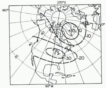
Fig. 7 Departure of the reconstructed annual mean 500 mbar height field for 18 ka BP from present climatology. Contour interval: 10 dm.

Vorticity fluxes cannot be computed directly from a time-averaged 500 mbar height field, and so are derived by an analog method. Based on the similarity between observed seasonal 500 mbar height departures and the ice-age reconstructions, the analog seasons chosen are the fall and winter of 1976 to 1977, and_ the spring and summer of 1958. The Greenland (positive) and Great Lakes (negative) anomaly centers in the . analog seasons are about a third the magnitude of those during the ice age (Fig.7). A first attempt at reconstructing vorticity fluxes, therefore, simply tripled the vorticity flux anomalies (i.e. the vector departure from the 34-year average) for each of the analog seasons. However, this created an improbable reversal of the direction of motion of the storm track off south-east Greenland. Multiplying the analog season vorticity flux anomalies by 1.7 yielded reconstructed ice-age vorticity flux fields (Fig.8) that are consistent with the reconstructed mean 500 mbar fields. The outstanding features of this reconstruction are a marked weakening of the storm track south and east of Greenland, a relative strengthening of the storm track over Baffin Island and southern Baffin Bay, and an absolute increase in this storm track over northern Baffin Bay, northern Greenland, and into the polar basin. Cyclone activity over the central Greenland ice sheet is reduced to nil.

Fig. 8 Reconstructed annual mean for 18 ka BP. Meaning of arrows as in Figure 1.

Atmospheric moisture content

Correlation of climatological mean dewpoints and thicknesses for various Greenland stations and seasons gives a dewpoint change of 3°C per 100 m. This value is applied to Lamb and Woodroffe’s ice-age thickness departure fields to give summer and winter ice-age dewpoint departures (spring and autumn are interpolated) from present climatology (e.g. Fig.9). The ice-age moisture content is computed from these adjusted dewpoints.

Fig. 9 Departure of reconstructed annual mean 500 mbar dewpoint temperatures for 18 ka BP from present climatology. Contour interval: 2°C.

Surface terrain

Surface terrain during the ice age (Fig.10) is assumed to be unchanged from the present for Greenland, Ellesmere Island, and Iceland. A continental ice sheet approximating that modeled by Reference Budd and SmithBudd and Smith (1981) for 18 ka BP is placed over the Canadian archipelago, with heights rising from sea level along the coast of Baffin Island to nearly 5 000 m at the south-west corner of the grid (northern Hudson Bay).

Fig. 10 Smoothed terrain used in the accumulation model; 1 km contour interval. Estimated conditions for 18 ka BP are shown; these differ from present terrain only in the south-western corner of the map.

Results

The reconstructed annual precipitation rate for the Greenland region is shown in Figure 11, and is shown as a percentage of the 1946–79 average model precipitation in Figure 12. Because of the calibration problems noted earlier, the accumulation percentages in Figure 12 should be considered more reliable than the calculated accumulations in Figure 11. Decreases of 60% during the ice age are widespread over the southern half of Greenland, and the 7 cm accumulation rate at the center of the ice sheet is but 30% of the present model value. In general, about a third of the decreases are due to reduced atmospheric moisture content; most of the rest is due to the weaker storm activity. The 70% decrease over south-eastern Baffin Island is largely due to orographic descent of storm systems from the continental ice sheet. While still somewhat below present values, ice-age accumulations over northern Greenland show an increase relative to the southern two-thirds of the island. In extreme northern Greenland the strengthened storm track just offsets the moisture decrease to produce a small area of slightly increased precipitation.

Fig. 11 Reconstructed annual precipitation distribution predicted by the accumulation model for 18 ka BP. Major contour interval: 20 cm water equivalent.

Fig. 12 Reconstructed annual precipitation for 18 ka BP, expressed as a percentage of 1946–79 average model precipitation for each grid point. Major contour interval: 20%.