1. Introduction: Theform and Structure of Former Ice Sheets

Early theories of ice-sheet form and flow (Reference NyeNye, 1951) envisaged ice sheets as non-streaming flows in which ice-sheet form, temperature and velocity distribution were functions of mass balance, surface temperature and radial distance from the ice divide. The first glaciological reconstructions of former ice sheets (Reference Boulton, Jones, Clayton, Kenning and ShottonBoulton and others, 1977 (British ice sheet); Reference SugdenSugden, 1977 (Laurentide ice sheet)) used these theories to reconstruct slowly flowing ice domes in which ice velocities were primarily a function of radial distance from the divide. Reference Boulton, Jones, Clayton, Kenning and ShottonBoulton and others (1977) admitted that their reconstruction could not explain the lobe that is believed to have existed at the glacial maximum down the east coast of England, which Reference Eyles, McCabe and BowenEyles and others (1994) later explained as a product of surging. Awareness of the importance of ice streams in the dynamics of modern ice sheets grew in the 1960s (e.g. Reference BauerBauer, 1961) and began to be reflected in thermomechanical models by the 1990s, when it became possible to include sufficient spatial resolution to capture the scale of streaming (e.g. Reference Payne and DongelmansPayne and Dongelmans, 1997).

Evidence of the profiles of former glaciers, based upon “trimlines” created by them along the sides of valleys through which, and on nunataks around which, they flowed, demonstrates that former ice sheets and ice caps in many areas had surface profiles that were very much lower than those predicted by classical theories. Reference MathewsMathews (1974) first demonstrated this for the southern flank of the Laurentide ice sheet, and Reference DykeDyke and others (2002) have collated data from which the maximum steepness of the profile of the western flank of the late-Wisconsinan Laurentide ice sheet is seen to have been much less steep than that of the Greenland ice sheet. These estimates reflect the maximum elevations to which the ice sheet extended, and could not have been produced by a surge. Reference Miller, Wolfe, Steig, Sauer, Kaplan and BrinerMiller and others (2002) have shown that the flow of the late-Wisconsinan ice sheet along the fjords of east Baffin Island was characterized by shear stresses of about 2–7kPa. This compares with shear stresses of 520 kPa along Antarctic ice streams (Reference Alley and WhillansAlley and Whillans, 1991), and with shear stresses of about 100 kPa in slowly flowing ice domes. Furthermore, geophysical Earth models used to invert relative sea-level data to infer ice loading suggest patterns of loading that are very different from those expected from classical glaciological models. For example, a glaciological model of the European ice sheet at the Last Glacial Maximum produced by Reference Denton and HughesDenton and Hughes (1981) suggested an ice thickness of up to 3400 m, whilst inversions of sea-level data by Reference Lambeck, Smither and JohnstonLambeck and others (1998) indicate thicknesses not in excess of 2000 m.

These observations are compatible with the suggestion of Reference Boulton and JonesBoulton and Jones (1979) that soft sediment deformation in the low-lying sedimentary zones that surround old, hard rock areas in Europe and North America permitted the ice sheet to flow readily at low shear stresses and with low profiles. This would produce the “Mexican hat” form modelled by Reference Boulton, Smith, Jones and NewsomeBoulton and others (1985), Reference Fisher, Reeh and LangleyFisher and others (1985) and Reference Clark, Licciardi, MacAyeal and JensonClark and others (1996), with a central, relatively steep zone associated with high basal friction and a peripheral low-friction zone. However, Reference Boulton, Dongelmans, Punkari and BroadgateBoulton and others (2001b) have suggested in the case of the European ice sheet that there is evidence of widespread streaming, and that low-profile streams with intervening high-profile, non-streaming zones would create an ice sheet with a low average thickness which could be compatible with sea-level inversions (Reference Lambeck, Smither and JohnstonLambeck and others, 1998).

Such an approach shifts perspective, from one in which we expect dominantly longitudinal variations in glaciological and glacial geological properties to one where there is strong transverse variation.

This paper explores the concept of streaming in former ice sheets, using the example of the European ice sheet: whether streaming can explain the evidence of low profiles, whether streams are forced or self-organized features of the ice sheet, and whether the sliding/non-sliding dichotomy plays an important role in the location of streams. It also illustrates the value of computational modelling, in permitting us to conduct experiments that nature does not allow.

2. Streaming in Former Ice Sheets: The European Example

Figure 1 shows a reconstruction of the axes of ice-stream development in the European ice sheet during and after its maximum, Late Weichselian extent. It is based on data from Reference Houmark-NielsenHoumark-Nielsen (1987), Reference Boulton, Dongelmans, Punkari and BroadgateBoulton and others (2001b) and Ringberg (in press). The stippled swathes do not show the lengths of ice streams at any one time, but the axes along which streaming was active during decay. It is difficult to assess the instantaneous lengths of ice streams, because of the time-transgressive nature of the geological evidence. However, Reference Boulton, Dongelmans, Punkari and BroadgateBoulton and others (2001b) suggested that stream D in Finland was 250–400km in length at 11200years BP, that ice stream C developed at 11300years BP, growing at the expense of streams B and D, that the latter ceased to function after 11200 years BP, that streaming ceased in C at 10 900 years BP and that its length just before it ceased to function as a stream was about 250–300km.

Fig. 1. Inferred axes (dark stipple) along which ice streams developed during European ice-sheet retreat after the Last Glacial Maximum. Heavy lines show ice-stream axes where the margins are uncertain. Concentric lines show the pattern of ice-sheet margin retreat. The ice-stream axes do not show the length of ice streams at any one time, but the swathes along which they perennially developed. The figure is based on data from Reference Houmark-NielsenHoumark-Nielsen (1987), Reference Boulton, Dongelmans, Punkari and BroadgateBoulton and others (2001b) and Ringberg (in press).

Several important conclusions can be drawn from this evidence:

We now use a glaciological model to investigate the streaming phenomenon in Europe, in order to investigate:

3. The Ice-Sheet Model

The model is based on that of Reference Boulton, Payne, Duplessy and SpyridakisBoulton and Payne (1994), developed further by Reference Hulton and MineterHulton and Mineter (2000), and is fully described in those papers, apart from the treatment of coupling between the ice sheet and lithosphere, which is described below.

3.1. The Earth model

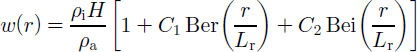
The evolution of the ice sheet is strongly coupled to the isostatic response of the Earth system. The Earth model is based on that of Reference Lambeck, Johnston and NakadaLambeck and others (1996) incorporating an elastic lithosphere and fluid asthenosphere. The downward deflection w(r), due to a load q of a thin plastic plate with thickness h and a flexural rigidity d floating on a non-viscous medium with density p_a, can be written as (Reference Lambeck and NatibogluLambeck and Natiboglu, 1980; Reference Le Meur and HuybrechtsLe Meur and Huybrechts, 1996):

(1)

where ∇_H is the horizontal gradient operator and g is the gravitational acceleration.

This is solved for a uniform disc load of density _Pi, height H and radius A for r ≤ A:

(2)

and for r≥A:

(3)

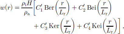
where the functions Ber(x),Bei(x), Ker(x) and Kei(x) are zeroth-order Kelvin functions. L _r = [D/(p_ag) ^1/4 is the radius of relative stiffness.

The resultant sea-level change, Δζ , is a function of geographic position (φ,ν), time t, and is dependent on the changes of ice distribution and the Earth’s response function. Sea-level change can be expressed as the sum of each ice sheet’s contribution to sea-level change:

(4)

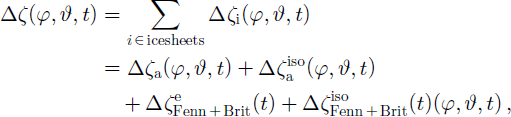
where Δζ_Fenn and Δζ_Brit are the contributions due to the European and British ice sheets and Δζ _a is the sum of the contributions due to all the other ice sheets.

3.2. Parameters that influence ice thickness

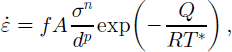
The average driving stress for ice-sheet flow is approximately given by the product of ice thickness and surface slope. If there is a strong flow response to this stress, the product of slope and thickness can be small compared to areas where the flow response is weak. The ease with which an ice sheet flows thus has an important influence on ice profile and thickness, and is itself strongly influenced by conditions at the basal boundary. The model employs a simple binary basal boundary condition. When the basal ice temperature is below the melting point, it adheres to its bed and it is assumed that no basal décollement occurs (we use the term décollement to include both basal sliding and deformation in subglacial sediments). If the bed is at the pressure-melting point, it is assumed that there will be décollement. At the melting point, the décollement velocity is proportional to a power of the gravitational driving stress:

(5)

with n = 3 (Reference PatersonPaterson, 1994) and the constant of proportionality a run-time parameter.

This approach does not depend upon a physical description or analysis of conditions at the basal boundary, but simply acknowledges that basal décollement in some form plays an important role in glacier dynamics. There is strong evidence (e.g. Reference Iverson, Jansson and HookeIverson and others, 1994) that subglacial drainage plays an important role in controlling the décollement process. If subglacial drainage of meltwater is inefficient, water pressures at the basal boundary will tend to be higher than if drainage is efficient. Most observations and analyses of movement at the basal boundary have concluded that the effective pressure at the ice/bed interface is an important determinant of movement, and, indeed, that variations in water pressure may cause temporal shifts between sliding and sediment deformation (e.g. Reference Fischer and ClarkeFischer and Clarke, 1997). High melting rates and poor drainage are likely to produce easier décollement and thus to reduce surface profiles for a given mass balance. Unfortunately, an improved analysis depends upon a theory of drainage, which although an object of much current study, is as yet not available in a tractable form.

An ice sheet can also be flattened by softening the ice. The flow law for thermally activated, isotropic flow is:

(6)

where is the strain rate, f a tuning parameter, a a material constant, σ the differential stress, d the grain-size, q the activation energy for creep, r the universal gas constant and t* the temperature corrected for the pressure-melting point. Glen’s flow law for polycrystalline ice is a special case of Equation (6), where the grain-size exponent p = 0 and n = 3. The remaining parameters are set to standard values (Reference PatersonPaterson, 1994): for cold ice (T*<263.15K) a= 1.14 × 10^–5 Pa–³ a–¹, Q = 60kJmol^–1 and for warm ice (T* >263.15K) A = 5.47×1010 Pa–3 a–1, Q = 139kJmol–1. Reference Tarasov and PeltierTarasov and Peltier (1999) report that the parameter, f, that determines the sensitivity of flow to temperature must be set to values as high as 80 to reconcile modelled ice sheets at the Last Glacial Maximum (LGM) with geophysical reconstructions based on isostatic adjustment. The ice sheet can therefore be flattened by increasing the overall ice temperature or increasing the value of the tuning parameter f. We have initially used a value for f of 80.

3.3. Experimental set-up

Initial bedrock topography is taken from the ETOPO5 and GTOPO30 datasets projected onto an Albers Equal Area Conic projection with a 10 and 5 km resolution. Global sea levels for the periods that are simulated are indirectly derived from the SPECMAP experiment (Reference Goodess, Watkins and PalutikofGoodess and others, 2000). Ice-sheet variations are forced by temperature and mass-balance distribution. Temperatures over the ice sheet are based on data from the Greenland Icecore Project (GRIP) ice-core record (Reference JohnsenJohnsen and others, 1992) adjusted by using palaeotemperature records from Europe in a way described by Reference Boulton, Dobbie and ZatsepinBoulton and others (2001c). The magnitude of local mass balance varies as a function of continentality, which is derived from the temperature function. The equilibrium-line altitude (ELA) is used as a free parameter, and is used to force the ice sheet so that it varies in the way that Reference Boulton, Dongelmans, Punkari and BroadgateBoulton and others (2001b) suggest is a reasonable estimation of the geological evidence of change through the last glacial cycle along a transect from the ice-divide region of western Sweden to the LGM position of the margin in northern Germany (Fig. 2).

Fig. 2. (a) The ELA variation required to create the pattern time/distance ice-sheet fluctuation during the last glacial inferred from geological evidence (Boulton and others, 2001 to have occurred along a transect from the Scandinavian tains, where the ice sheet was initiated, to northern Germany. ( b) Temperature functions based on the GRIP record (Reference JohnsenJohnse and others, 1992) that are used as model drivers. The warmer function is used to derive simulations 1–3 and 5.The colder function is used to drive simulation 4. (c) The geologically inferred pattern of variation of the ice-sheet margin along transect (upper line) compared with the modelled variation driven by the ELA in (a) and a temperature function based on the GRIP record (Reference JohnsenJohnsen and others, 1992).

We now explore the impact on ice-sheet streaming of the form of the bed, the temperature of the ice mass and the sliding/non-sliding condition at the bed.

4. Ice-Stream Development on A Smoothed Bed (simulation 1)

Reference Payne and DongelmansPayne and Dongelmans (1997) have demonstrated that the “creep instability” identified by Reference Clarke, Nitsan and PatersonClarke and others (1977) resulting from the temperature dependence of ice flow can create self-organized streaming where ice flows over a flat, homogeneousbed. They suggested that the instability which in a flowline model leads to temperature-driven oscillations of the margin (Reference Boulton, Payne, Duplessy and SpyridakisBoulton and Payne, 1994) is accommodated in a three-dimensional model by spatial shifts in the location of streaming. Reference Hulton and MineterHulton and Mineter (2000) undertook similar experiments and showed that streaming was a way in which the of ice-sheet flow system adjusted to the mass balance and temperature cycle drivers of flow as basal temperatures increase towards b) the melting point. They showed that an increased mass-mounbalance flux can be accommodated by an increase in the number of streams and that streams will tend to widen down-n ice in order to discharge the down-ice increase in the mass-balance flux. They showed that the introduction of depressions on the bed permitted greater warming, leading to basal melting occurring there earlier than elsewhere, and therefore the that the pattern of initial streaming was strongly conditioned by bed topography.

In explaining the streaming features of the European ice sheet and the questions posed in section 2, we wish to understand the extent to which dynamic features are forced by the topographical characteristics of the bed. In order to explore this, we first examine the streaming produced on a smoothed European surface and then compare it with the streaming developed over a realistic European topography when the ice sheet is forced by the same climate function.

We retain a smoothed version of the Scandinavian mountain chain as a nucleation zone for the ice sheet, completely smooth the flanking lowland and continental-shelf zones, but retain a sharp marine margin for the continent to halt the seaward growth of the ice sheet. The bed is smoothed by a three-node running mean in all directions at elevations 41000 ma.s.l. At lesser elevations, and down to –300m a.s.l., the bed becomes a flat surface with an elevation of 0 m a.s.l. A smooth function connects the bed above 1000 ma.s.l. and that at 0 m. The ice-sheet model is then driven by the temperature and ELA variations shown in Figure 2. Figure 3 shows the extent of the ice sheet at 40 000 years BP, and the basal temperature corrected for pressure melting. It shows that even where the bed is flat, creep instability creates streams along which melting-point temperatures, and therefore sliding, occur earlier and further up-flow than in intervening zones. Figure 4a shows the pattern of streaming along a transverse transect across the zone of inter-fingering of cold/warm ice in the southeastern sector of the ice sheet shown in Figure 3.The streams in this sector of the ice sheet are 1–12 km wide, compared with observed widths an order of magnitude greater during ice-sheet decay at times when the ice sheet had a similar extent. There is a strong contrast in the model between the northern and southern sectors of the ice sheet. Figure 4b shows surface flow velocities and bed and ice surface topography along a transverse transect on the northern flank of the ice sheet at elevations below sea level where the smoothing function has not been applied (Fig. 3). Relatively wide streams (50 km) and inter-stream ridges develop in response to bed irregularities, although the streams persist far into the zone where the bed has become flat. Rather than developing freely as an unconstrained, self-organized response of the ice sheet to creep instability as they do in the southeastern flat-bed zone, the first-formed streams in the north occur where the bed is locally lower, the ice thicker and melting first occurs, creating a strong feedback between temperature and flow. Once a stream has formed, it tends to perpetuate itself downstream even in the flat-bed region. A stable mass flux is maintained in the southern sector by a large number of self-organized narrow streams, and in the northern sector by a small number of broad, bed-influenced streams.

Fig. 3. Simulation 1 showing the spatial variation of basal temperature at 40 kyr BP in the ice-sheet model driven by the ELAfunction in Figure 2a over a smoothed European surface. Red shows warm ice, yellow and green cold ice.The spiky penetrations of warm ice in the distal zone into cold ice in the proximal zone indicate the locations of ice streams. Contour lines are in white at 500 m intervals.The streams in the southeastern sector have developed spontaneously on a flat bed.The broad streams in the north reflect the forcing effect of residual valleys in the mountain belt and below ^300 m.The heavy lines transverse to flow show the locations of transects in Figure 4.

Fig. 4. Simulation 1 results. (a) The locations of streams, indicated by velocity variations (spiky line) along the flow-transverse transect shown in Figure 3 in the southeastern sector of the ice sheet. The smoother lines are the elevation of the ice-sheet surface and bed. (b) Wider streams on the northern flank of the ice sheet. Isostatic depression of the bed in this sector has taken it below the smoothing cut-off at –300 m, so that valleys occur in the bed (smoothed lower line). The streams reflect both valleys at this depth and coaxial valleys above 1000 m. Forcing by bed topography can clearly override self-organizing tendencies such as those reflected in the southeastern sector of the ice sheet.

5. Ice-Stream Development Ona Realistic Bed (simulation 2)

In this case, the initial bedrock topography is not smoothed. The ice-sheet model is again forced by the temperature and ELA function shown in Figure 2. This is designed to produce a pattern of time-dependent ice-sheet fluctuation along a transect from central Sweden to northern Germany similar to that inferred from the geological record (Reference Boulton, Dongelmans, Punkari and BroadgateBoulton and others, 2001b). The details of ice-sheet advance and decay are different from those created at similar times using the smoothed model (Fig. 2). Figure 5 shows melting at the base of an ice sheet of extent similar to that of the smoothed model in Figure 3.The patterns are quite different:

Fig. 5. Simulation 2 showing the distribution of temperature at the base of the ice sheet flowing over a realistic bed at 80 kyr BP, when the ice sheet had an extent similar to that of the smoothed-bed ice sheet in Figure 4 and was driven by the same climate.The zones of melting in red colours are zones of streaming.The colour code is the same as in Figure 3. Contour lines are in white at 500 m intervals. Deep valleys strictly control the width of streams in the mountainous western sector of the ice sheet, but streams coalesce into broader features on the continental shelf. In the southeastern sector, where the topography is muted, a very large stream occupies the Baltic basin and broad fan-like streams occur in southern Finland (compare with actual features in the same area in Figure 1).

The width of streams is up to an order of magnitude greater, in the southeastern sector in particular, than in the smoothed model. It is also noticeable that similar patterns are generated by the model during successive stadial periods of the last glacialcycle, although the rates of basal melting vary considerably. We conclude therefore that basal topography is a major determinant of the precise pattern of streaming that the ice sheet adopts to ensure abalanced flow response to the mass-balance flux. Not only does streaming reflect topography, but in some areas, such as in southern Finland, rather than reflecting local topography, streaming appears to reflect the locations of valleys on the Gulf of Bothnia coast of northwest Finland. We suggest that the axes of streaming that developed in northwest Finland were sustained, as the ice sheet advanced, as a memory effect into southern Finland, which helps to explain why axes of streaming tend to be relatively stable through time even though the bed is of very low relief.

Streams in areas of low relief that are not confined by steep valley walls tend to fan out down-flow, supporting the contention of Reference Hulton and MineterHulton and Mineter (2000) that this could be a reflection of the way in which the ice sheet balances the increasing down-ice flux. We suggest that where ice streams are relatively unconstrained by valley walls, the greater width of the streams in the European ice sheet compared with those of Antarctica may reflect the higher average internal temperatures in the former,

Where streaming is intense because of a deep subglacial trench and a strong, convergent ice flux into the stream, highly elongate lobes can form. This is the setting of the ice stream that is believed to have developed along the Norwegian Channel (Reference Sejrup, Larsen, Landvik, King, Haflidason and NesjeSejrup and others, 2000; and A in Fig. 1). The Channel extends from the Skagerrak, in the vicinity of Oslo Fjord, and extends as far as the continental-shelf edge. It is up to 60 km wide, with abase extending down to 300 mbelow modern sea level. Our simulation of the ice stream along the Channel (Fig. 6) shows a highly lobate form, consistent with the geological evidence (Reference Sejrup, Larsen, Landvik, King, Haflidason and NesjeSejrup and others, 2000).

Fig. 6. Detail of a modelled ice stream (simulation 2) along the deep trough of the Skagerrak and Norwegian Channel at 20 kyr. The colour fringes show surface velocities (blue–green: slow; yellow–red: fast), and arrows show surface velocity vectors. Contour lines in white at 250 m intervals. The strongest flow occurs along the axis of the Channel, but ice spills over its southern flank, and could have been responsible for transporting the observed erratics from the Oslo region into Denmark (Reference Houmark-NielsenHoumark-Nielsen, 1987). The over-riding of the Jaeren area in southwest Norway (the grey area of land to the east of the Norwegian Channel ice stream) by the ice stream before it was over-ridden by inland ice is confirmed by local geological evidence (e.g. Reference Sejrup, Larsen, Landvik, King, Haflidason and NesjeSejrup and others, 2000).The ice divides are clearly shown. Notice the convergent flow of ice into the heads of streams near to ice divides.

6. The Impact on Streaming of Ice-Sheet Properties (simulations 3–5)

Although we have shown that the form of the bed can play a fundamental role in governing the location of streaming and the width of streams and their stability, ice-sheet properties may also play an important role in governing the flow regime. The properties that we believe could have a first-order effect on flow are:

Using the realistic bed, we now explore, in simulations 3–5, the impact on streaming of changing the above ice-sheet properties as follows:

1. 3. Suppressing basal décollement even when the ice/bed interface is at the melting point, but with the same temperature driver as in simulations 1 and 2. This is done by not applying the sliding condition (Equation (5)) when the basal temperature rises to the melting point.

2. 4. Lowering the temperature driver such that the ice sheet is much colder and almost all the ice/bed interface is below the melting point. We reduce the driving temperature at the surface of the ice sheet (Fig. 2b) by 10°C.

3. 5. Changing the value of the flow-sensitivity parameter from 80 to 20, but using the same temperature driver as in simulations 2 and 3.

Figure 7 shows the basal temperature distribution for simulation 4, the cold condition with very limited basal melting, at 85 kyr. Compared with Figure 5 (simulation 2), it shows narrow and restricted zones of streaming and basal melting, except on the western coast of Norway where valley-bound streams spread out and coalesce on the continental shelf. Figure 8 compares streaming patterns in simulations 2 and 4 by showing the 100 ma^–1 surface velocity contours for time slices at 90, 85 and 90 kyr.We suggest that the narrower streams of simulation 4 reflect the limited width of the streams required to balance the flow when ice temperature is low. The precise initiation locations are, however, still determined by bed topography, and in some cases local melting occurs in the bottoms of valleys. The concentration of warmer ice at stream-initiation points in topographic lows leads to advection of warm ice so that warm streams are sustained down-glacier even when the topography appears inimical to streaming.

Fig. 7. simulation 4 at 85kyr, showing the distribution of basal temperatures and the surface elevation contours at 500 m intervals (white lines). the surface temperature of the ice sheet is lowered by 10° c, so that the internal temperature is low and basal melting occurs at only afew locations in deeper areas of the bed. ice streams in the southeastern sector are very narrow compared with those in simulation 2 (fig 5). the heavy line in the southern sector of the ice sheet shows the location of the velocity and elevation cross-sections in figure 9.

Fig. 8. The growth of the ice sheet at 90, 85 and 80 kyr shown by the successive ice-sheet margins (marked in black) and the development of ice streams. These are represented by red line showing the successive positions of the 100 m a–1 surface velocity contour. Up-glacier deflections show zones of rapid flow. (a) Results for simulation 2 (realistic bed, high surface temperature, basal decollement at the melting point). Streams are relatively broad and are sustained for the whole period. (b) Results for simulation 4 (low temperature, little basal melting). Streams remain very narrow.

Simulation 3 (not figured), in which decollement is prevented, shows a condition intermediate between simulations 2 and 4. In simulation 5 (not figured), where the f factor is reduced from 80 to 20, streaming is relatively suppressed. In all cases, similar patterns of streaming are generated by the steep-sided valleys in the Scandinavian mountains, although the cold case tends to generate narrower streams.

Figure 9 shows a transverse cross-section of surface velocity (Fig. 9a) and ice surface and bed elevation (Fig. 9b) along the line shown in Figure 7 at 85 kyr. The cold case has a limited number of narrow zones of melting associated with relatively fast, narrow (3–8 km) streams, and a low average velocity compared with other cases. These very strong contrasts reflect the fact that in simulation 4, colder ice requires fewer, narrower streams and the flow mechanism changes across the molten/frozen interface, whereas there are no such changes in simulation 3 (no décollement) or simulation 2 (widespread melting). In simulation 5, the reduction of the temperature sensitivity of flow reduces the creep instability and tends to suppress streaming.

Fig. 9. Ice-sheet surface velocities (upper diagram) and ice surface and bed elevations for the line of section shown in Figure 7 and for simulations 2–5.

It is noticeable that in the shallow depression of the Baltic (Fig. 9b), simulation 2 in particular shows a very broad stream (30–70km), with maximum velocities of 250ma^–1 compared with velocities of about 140 m a^–1 on its western flank, although with minor velocity peaks that reflect small-scale undulations of the bed. In any one transverse section, streams do not necessarily correspond to bed depressions, because of the thermal memory effect.

The ice-thickness contrasts in these simulations (Fig.9b) reflect the fact that cold ice is more sluggish than warmer ice, and demonstrate that streaming has a significant effect on ice thickness, that a reduced temperature sensitivity inhibits streaming and that the absence of basal décollement reduces streaming compared with the cases in which décollement is permitted. Although décollement does make a difference, reducing ice thickness in Figure 10 by up to 250 m (19%) compared with the no-décollement case, the effect of Equation (5) is smaller than might have been supposed, reflecting the effectiveness of the creep instability mechanism even when sliding is suppressed.

6. The Nature of Basal Decollement

Although we have explored the impact of basal décollement on streaming behaviour, we have done so by using the common, but arbitrary, assumption that décollement is proportional to a power of the driving stress where the bed is at the melting point. There is strong evidence, however, that two other important controls, which could be at least as important as driving stress, need to be taken into account:

Both these sets of processes depend upon the character of the bed (e.g. Reference Clark and WalderClark, and Walder, 1994). It is premature to explore their potentially strong impact until we are able better to formulate a physically based model for them. But their investigation is an important priority. In the case of the European ice sheet, the distribution and character of unlithified sediments overlying bedrock may play an important role in determining areas of easy flow. Much such sediment lies in low points of the topography, where it could lead to even easier flow than in our model.

7. Conclusions

1. 1. Ice streams played a vital role in determining the dynamics, form and thickness of the European ice sheet during the last glacial cycle. The principal axes of streaming were relatively stable.

2. 2. On an artificially smoothed bed, simulations suggest that ice streams develop as parts of an unforced, self-organizing pattern of flow that permits the ice sheet to adjust to its mass-balance flux. They are a consequence of a thermally controlled creep instability.

3. 3. On a smoothed bed, streams are created that are as much as an order of magnitude narrower than geologically inferred streams in the last European ice sheet.

4. 4. Simulations ofa relatively warm ice sheet, which reaches the melting point over large areas of a realistically rough bed, creates ice streams that are of similar dimensions to those inferred for the European ice sheet. The form of the bed plays a fundamental role in determining the locations of streams. Their initiation is largely determined by low points in the bed where basal ice tends to be warmer. Much of their subsequent evolution is predetermined by their early history, which may account for the relative stability of the principal axes of streaming in the European ice sheet.

5. 5. Simulated flow of very cold ice over a realistically rough bed produces very narrow streams. We suggest that this occurs because the thermal creep instability is relatively suppressed, and because highly localized basal melting permits local basal décollement which helps to sustain streaming.

6. 6. Although basal décollement of ice at the melting point produces a strong feedback that enhances streaming, essentially similar patterns of streaming are created in simulations in which décollement is arbitrarily prevented. The creep instability in extensive, warm-based ice can create streams almost as broad as those created when décollement is permitted.

7. 7. Streaming is a means whereby large ice fluxes can be sustained under low driving stresses. As a consequence, it can play an important role in maintaining a low-thickness ice sheet. For the European ice sheet, we estimate that a relatively warm ice sheet with broad streams can reduce the maximum ice thickness by >1 km compared with a cold ice sheet with narrow streams.

8. 8. It is premature to draw conclusions about the role of basal décollement until we are able to develop a drainage theory coupled to sliding theories for both rigid and deforming beds, although we believe that the extensive areas of glacially deformed, unlithified sediment in Europe had an important impacton flow.