1. Introduction

GPS kinematic and static measurements and radio-echo-sounding (RES) surveys were carried out in the framework of the European Project on Ice Coring in Antarctica (EPICA), Dome Concordia (Dome C) project, in order to examine the glacier dynamics thoroughly. As ice flow is related not only to the ice properties but also to ice thickness and bedrock slope, a precise surface morphology is needed to detect the ice divide and the main ice-flow directions.

During the 1993 Dome C French-Italian Antarctic campaign, an initial kinematic global-positioning-system (GPS) survey was performed using two geodetic LI frequency Trimble 4000SE GPS receivers. The GPS surveys evaluated height variations over a 1500 km² area, in order to localize the topographic dome where the 4 km drilling was to be undertaken.

A morphological map, obtained from radar-altimeter data (Reference Brisset and RemyBrisset and Remy, 1996) was first used to localize a position on Dome C (75°09′S; 123°06′E). In summer 1993, a French DORIS (Determination d’Orbite et Radiopositionnement Integres par Satellite) antenna was installed at this location (Reference VincentVincent, 1994) to obtain the absolute geographic coordinates with an accuracy better than 0.10 m (World Geodetic System WGS84 coordinates: 75°09′09.8794" S, 123°05′ 55.2725" E; 3232.772 m a.s.L). The first base station for the kinematic GPS survey was near the DORIS antenna, at the above location. A second GPS receiver, mounted on a snow tractor (Challenger DV87), was used as a rover. GPS survey profiles were star-shaped, centered on this position (Fig. 1).

Fig. 1. The GPS surveys: 1993 kinematic survey, centered on the first approximate Dome C location (light blue); 1995 (A) kinematic survey (red); and 1995 (B) kinematic survey (blue), both centered on the new Dome C location. The triangles represent the points of the geodetic network. The circular symbols refer to the tested cross-overs between the different kinematic profiles. Coordinates are UTM from WGS84 ellipsoid: central meridian 12? E The corresponding WGS84 eliPsoid coordinates of the four vertices relative to grid limits are shown.

The integration of the carrier-phase data with radar-altimetric data from the European Remote-Sensing Satellite (ERS-1) (performed by F. Remy, Groupe de Recherche de Geodesie Spatiale, Tolouse) provided coordinates of the maximum elevation site for the subsequent topographic and geophysical surveys (Reference Cefalo, Tabacco, Manzoni and UnguendoliCefalo and others, 1996). The resulting location (Table 1) is approximately 11 km northeast of the initial Dome C position.

Table 1. Elipsoid and plane UTM coordinates of Dome C obtained from the analysis of the 1993 kinematic GPS data

2. RES and GPS Surveys in 1995/96

Kinematic GPS and RES surveys were carried out during the 1995/96 Antarctic campaign to investigate the topographic surface and bedrock topography. A star-shaped grid, centered on the new Dome C location (kinematic survey A, Fig. 1), was surveyed in conjunction with a ground RES survey (Reference Tabacco, Passerini, Corbelli and GormanTabacco and others, 1998). Other kinematic GPS profiles, covering an area of about 2000 km² (Reference Gandolfi, Vittuari and UnguendoliGandolfi and Vittuari, 1996) (kinematic survey B, Fig. 1), were also carried out.

Sixty MHz airborne and ground-based radar measurements were made on three grids. The first, a 80 km × 120 km rectangular grid with 10 km spacing between flight lines, was centred on the summit point, with the longer side parallel to the apparent dome axis. The second, a 50 km × 50 km square grid with 10 km line spacing, was concentric with the previous one, but shifted by 5 km from the lines of the "big grid" in order to obtain a final coverage in the central part of the area with a spacing of 5 km between the flight lines. The third, ground-based survey, was made up of six right-angled isosceles triangles, with the perpendicular lines 10 km long, rotated from each other by 60°. The total airborne survey length was about 2800 km. The ground-based one was about 300 km. Ice thickness over the whole area was calculated and the bedrock map constructed.

The following main bedrock features were detected:

1. (a) a plateau located in the central part of the area at a mean elevation corresponding to zero height-above-elipsoid (HAE);

2. (b) a sharp ridge, near 125° E, oriented south-north which is probably a tectonic feature. At 124.5° E, an important trough, more than 500 m deep, yields a gradient up to 1000 metres per two kilometres; and

3. (c) a southern chain of mountains, oriented eastward, that probably diverts the flow coming from Vostok. The presence of a dome in this area is due to these two chains of mountains that influence the ice flow.

During the same campaign, a GPS geodetic strain network was established over an area of about 2000 km² (Reference Gandolfi, Vittuari and UnguendoliGandolfi and Vittuari, 1996). The network consisted of 37 points, distributed symmetrically on four concentric rings centered on the DORIS point (Fig. 1). Its geometry was simulated and analysed for optimization (Reference Gubellini, Radicioni, Stoppini and UnguendoliGubellini and others, 1996). 120 mm diameter aluminum stakes, 3 m long, inserted at least 2 m in the snow were adopted for the vertices.

Geodetic Trimble 4000 SSE and SSI L1/L2 receivers were used for the kinematic surveys, using high sampling rates to allow a detailed survey of the altimetric profiles. Pseudo-range and carrier-phase data on both frequencies were stored by all receivers at every epoch. The recording time at stations was approximately 20 min, and varied with respect to the distance between the master and rover receivers.

One or more GPS receivers were located as reference on the vertices of the geodetic strain network. The rover receivers, equipped with geodetic antennas, were installed on tracked vehicles. The reference stations were installed at the nearest vertices of the strain network to obtain the best kinematic GPS solution. The whole track length during the kinematic surveys was about 420 km.

Static acquisitions (20–30 min long) were performed to compute the sets of initial integer-ambiguity parameters at the beginning of each kinematic survey. Other stops on particular tracts of the trajectories were planned to improve data processing. Comparison between the tracts of the kinematic trajectories and the points of the geodetic strain net allowed the accuracy to be checked.

3. GPS Data Processing

In equatorial and auroral areas, anomalies in the structure of the ionosphere cause a scintillation effect on the GPS signal. Such interference is particularly critical for high-accuracy GPS surveys because it creates cycle slips which make the integer estimation of phase ambiguities difficult. In other words, the signal-to-noise-ratio is degraded and an erroneous phase-cycle count may occur without apparent loss of lock (Reference ViterbiViterbi, 1996; Reference CiraoloCiraolo, 1994).

GPS data were preprocessed to check quality and identify problems. The use of multiple reference stations overcame particular problems regarding sets of static data affected by a large number of cycle slips on the L2 frequency. Kinematic data were processed using the static data of other receivers, simultaneously recording on the points of the geodetic network.

The rover-receiver trajectory was computed afterwards, using the GPSurvey software (Trimble) and the Geotracer GPS software v. 2.25 developed byTerraSat. The package included an on-the-fly (OTF) algorithm, mainly designed for airborne GPS, that could recover the cycle slips (Reference LandauLandau, 1989; Reference Euler and LandauEuler and Landau, 1992).

The OTF algorithm included in the Geotracer program has several steps. A preliminary solution using the code modulated on the GPS frequencies was scanned to locate an optimal observation time-span for ambiguity resolution. This OTF ambiguity solution was performed on each selected interval using the following procedure: a solution using float-carrier phase ambiguities for each satellite was estimated; estimated ambiguities were used to find a fixed solution; and the sets of ambiguities were statistically validated to guarantee the desired centimetric accuracy. Validated ambiguities were then fixed and propagated through the whole tracking time between losses of lock for each satellite.

Finally, the values of the relative-dilution-of-precision (RDOP) parameter relative to the processed data were analysed to overcome particular satellite-receiver geometries causing divergences in the double-difference system equations.

High values of the RDOP parameter can occur even with good positioning-dilution-of-precision (PDOP) values, considering that the RDOP value also depends on the relative position between the two GPS antennas:

where A is the coefficient matrix of the linearized double-difference system equations, is the variance-co-variance matrix of the phase measurements, and is the weight unit variance.

The complanarity of visible satellites, some other particular satellite geometry, or rover-master direction, create a singularity in the double-difference system equation, with altered values of matrices suddenly increasing the resulting value of the RDOP parameter.

A forecast of the RDOP parameter often helps avoid problems of divergences in the solutions. Software that calculates its value for pseudo-range and phase measurements, starting from the satellite almanac, was developed at the University of Trieste (Reference Cefalo, Manzoni and SkerlGefalo and others, 1995).

Validation of profile portions was performed using the initial and final static aquisitions and comparison with the strain-net vertex coordinates.

The 1995 kinematic surveys are plotted in Figure 1 together with the 1993 kinematic trajectories (in Universal Transverse Mercator coordinates). The repeatability of GPS measurements was estimated from cross-over errors. The analysis was performed by comparing the ellipsoid height values at the intersections between the different trajectories, for every kinematic survey and for the two different sets of kinematic data. Table 2 summarizes the results of this analysis for the intersection points shown in Figure 1.

Table 2. Results of the analysis performed on the intersections between the different kinematic profiles in Figure 1. The values represent the differences in metres between the ellipsoid height values at crossovers

4. Altimetric Contouring

GPS tridimensional coordinates obtained from the two kinematic datasets and the points of the geodetic strain network were used to build the topography of the Dome C surface. Four common types of interpolators (kriging, triangulation, inverse distance to a power and minimum curvature) were considered a priori and tested using the 1995 kinematic GPS profiles as source data, and the GPS network as test points, in order to choose the best interpolation method. Several options were used for each interpolator, varying the shape and size of the search radius for each gridding technique; the anisotropy for searching, the power for the inverse distance (2 and 3 power were used), as well as the level of smoothing. Each parameter was changed leaving the others constant. The residuals were then calculated for each grid obtained on the GPS static points. The standard-deviation parameter of whole residuals was computed for each grid. Table 3 summarizes the best values obtained for each gridding technique analysed. Based on these analyses, the "triangulation" gridding technique was chosen. The contour levels were plotted every 0.25 m with highly smoothed contours. This was done in order to obtain a smoother topographic surface. From the kinematic GPS it is possible to show the roughness of the surface, particularly the shape of sastrugi features created by katabatic winds, but this is only true on the surveyed profiles. An extrapolation of this "high-frequency" component of the surface would not be realistic elsewhere. A contour interval of 0.25 m was thus adopted based on the tested accuracy of the GPS data. The resulting map is shown in Figure 2.

Table 3. Comparison between the statistical parameters of the best results obtained for each gridding interpolator, using the 1995 kinematic profiles as source data and the static GPS points of the geodetic network as test points

Fig. 2. Done C topographic surface from 1995 GPS data using all kinematic (A and B) and static surveys (geodetic network). Contour interval is 0.25m.

The residuals between the grid obtained using 1995 GPS data and 1993 kinematic data were computed in order to test the range of height variations in the Dome C area between the two surveys. The values were in the range of accuracy of the 1995 grid. A new map was therefore drawn up using all the data (Fig. 3). The contour map (0.25 m interval) was computed inside the external perimeter of the geodetic strain network. The topographic surface was then used as reference for the bed topography obtained from ground-based and airborne radio-echo-sounding surveys. Figure 4 shows the bedrock topography of Dome C area. The topographic anomalies visible in the southwestern part of Figure 3 relate to the effects of the little ridge of the mountain chain, which acts like a barrier, and to ice fluxes coming from south, which can alter the features.

Fig. 3. The final surface map of Done C area obtained contouring all 1993 and 1995 GPS data. Contour interval is 0.25 m.

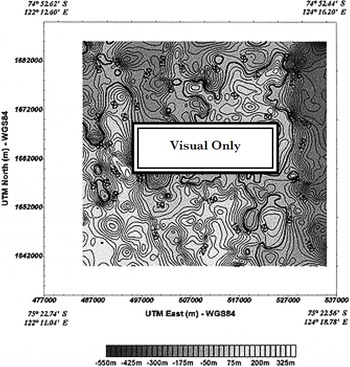
Fig. 4. Bedrock topography of Dome C area from radio-echo soundings. The asterisk identifies the Dome C location. Heights are WGS84 ellipsoid ones. Contour intercal is 25 m.

5. Conclusions

The 1993 kinematic GPS data and the 1995 static and kinematic data were used to map the topographic surface of the Dome Concordia area, with an accuracy in the range of 0.20 m. This value also takes into account the tracked-vehicle penetration into the ice between one passage and the next, whose value was evaluated in the range of 0.10 m. The resulting map can be considered as the Dome C topographic reference map for the 1995/96 austral summer.

The interferential kinematic GPS method is a quick and precise technique for surveying the topography of an area, and can synchronize and georeference data from different geophysical surveys. This technology gives accurate data that can be used alone, or in connection with other geophysical techniques, and is capable of covering larger areas, but requires a precise absolute calibration (i.e. ERS-1 radar altimeter).

The main advantages of the method are the high productivity and reliability of measurements, even in extreme environmental conditions. Comparison between different GPS techniques, characterized by different levels of precision, allows an internal validation of the results. Finally, the use of the contemporary French DORIS system allowed the whole GPS survey to be positioned into the adopted International Terrestrial Reference Frame (ITRF ’92) system, and then into the WGS84 ellipsoid at centimetric accuracy.