

1. Introduction
The meltwater from shrinking glaciers is a major contributor to global sea-level rise (e.g. (Hock and others, Reference Hock, Pörtner, Roberts, Masson-Delmotte, Zhai, Tignor, Poloczanska, Mintenbeck, Alegría, Nicolai, Okem, Petzold, Rama and Weyer2019; Oppenheimer and others, Reference Oppenheimer, Pörtner, Roberts, Masson-Delmotte, Zhai, Tignor, Poloczanska, Mintenbeck, Alegría, Nicolai, Okem, Petzold, Rama and Weyer2019; Horwath and others, Reference Horwath2022)) and regional hydrology (e.g. Huss and Hock, Reference Huss and Hock2018). Concern is also growing about possible water resource scarcity (e.g. Mark and others, Reference Mark2017), an increasing hazard potential from growing pro-glacial lakes (e.g. Furian and others, Reference Furian, Loibl and Schneider2021) and further adverse effects (e.g. destabilised mountain slopes, tourism) from ongoing climate change impacts on glaciers (e.g. Fernández and Mark, Reference Fernández and Mark2016; Hock and others, Reference Hock, Pörtner, Roberts, Masson-Delmotte, Zhai, Tignor, Poloczanska, Mintenbeck, Alegría, Nicolai, Okem, Petzold, Rama and Weyer2019). Thereby, knowledge about past glacier changes is key to improve our understanding of future glacier changes. For example, for a century-scale perspective of future glacier evolution, it would be good to have a perspective of the same length into the past. However, past glacier outlines in a digital vector format (e.g. shapefiles) are sparse and related comparisons rare. As the visibility of trimlines and moraines degrade over time due to vegetation recovery and continued erosion (e.g. Eichel, Reference Eichel, Heckmann and Morche2019), it will be increasingly difficult to properly map these features. Without this information it is also difficult to determine how large the glacier contribution to sea-level rise really was over the past century (Marzeion and others, Reference Marzeion, Jarosch and Hofer2012). Reconstructing past glacier extents by geomorphological interpretation of satellite images has already been performed (e.g. Meier and others, Reference Meier, Grießinger, Hochreuther and Braun2018) and has been used as a proxy for past climate conditions (Wolken and others, Reference Wolken, England and Dyke2008) or to determine how much glaciers contributed to sea-level rise (Glasser and others, Reference Glasser, Harrison, Jansson, Anderson and Cowley2011; Carrivick and others, Reference Carrivick2019, Reference Carrivick, James, Grimes, Sutherland and Lorrey2020; Lee and others, Reference Lee2021).
During the Little Ice Age (LIA), the latest cool period of the Neoglacial (Matthes, Reference Matthes1939; Porter and Denton, Reference Porter and Denton1967; Grove, Reference Grove2004), glacier advances all over the world created impressive lateral and frontal moraines, i.e. accumulations of unsorted stones, rocks and boulders that were deposited during phases of glacier advance or stagnation and left behind after the ice melted away (Benn and Evans, Reference Benn and Evans2010). The most recent of these moraines often leave sharp crests in the landscape that are clearly visible today. Trimlines are linear (or zonal) changes in vegetation, erosion pattern, material composition or slope along the former glacier margin that have also widely been used for reconstruction of former glacier extents (Cogley and others, Reference Cogley2011; Rootes and Clark, Reference Rootes and Clark2020). The differences in vegetation cover for terrain that has been ice-free for a long (a few thousand years) or a short time (a few hundred years) are often clearly recognisable, in particular on false colour infrared imagery showing healthy vegetation in reddish colours. Vegetation trimlines have thus also been used to determine former glacier extents, in particular for glaciers and ice caps that have not formed prominent lateral or end moraines (Wolken and others, Reference Wolken, England and Dyke2008). The missing vegetation cover and/or the often sharp crested walls of LIA moraines also allow a separation from much older Neoglacial moraines.
Mapping LIA glacier extents has long been carried out in the field, but the outlines on the related published maps (e.g. Grove, Reference Grove2004) are often not available in a digital vector format. With the availability of orthorectified satellite images and geographic information systems (GIS), glacier extents can be mapped directly in this format and shared with the community. Previous studies have revealed that Landsat-type resolution (15–30 m) is sufficient for the mapping if prominent moraines and trimlines are present (Kutuzov and Shahgedanova, Reference Kutuzov and Shahgedanova2009; Svoboda and Paul, Reference Svoboda and Paul2009; Loibl and others, Reference Loibl, Lehmkuhl and Grießinger2014; Tielidze, Reference Tielidze2016). Paul and others (Reference Paul2013) concluded that the precision of manual glacier delineation with very high-resolution (1 m or higher) images is not necessarily better than with Landsat (30 m), but Paul and others (Reference Paul, Winsvold, Kääb, Nagler and Schwaizer2016) argued that for glacial geomorphological mapping a higher resolution strongly improves the identification and interpretation of moraines or trimlines. Accordingly, the now available Sentinel-2 satellite images with 10 m spatial resolution offer a better view of these features than 30-m Landsat images. Baumann and others (Reference Baumann, Winkler and Andreassen2009) mapped LIA glacier outlines with high-resolution (0.4 m) aerial images as well as 30 m Landsat scenes and acknowledge the improved capabilities of identifying geomorphological features with higher resolution images. Also Leigh and others (Reference Leigh, Stokes, Evans, Carr and Andreassen2020) used very high-resolution orthophotos to map LIA glacier extents in northern Norway, confirming that spatial resolution plays a role to obtain good results.
With the increasing availability of Web Map Services (WMS) and the possible direct integration of the related very high-resolution (i.e. better than a few metres) imagery into GIS software such as ArcMap or QGIS, new doors are opening for digital mapping of former glacier extents based on geomorphological interpretation (Chandler and others, Reference Chandler2018). The so-called ‘World imagery’ layer is part of the ESRI basemaps and largely composed of GeoEye and WorldView scenes of up to 0.3 m resolution. These would have a high price tag if obtained individually over large regions and have thus only rarely been used for small-scale applications. Chandler and others (Reference Chandler2018) noted that some caution is needed when using the images provided by WMS, mostly because of errors in georeferencing and the often difficult determination of image acquisition dates. However, the latter point is less of an issue when mapping LIA extents, as geomorphological features do not change much over decades compared to the often very dynamic glacier margin. For example, Lee and others (Reference Lee2021) have used WMS imagery, mapping almost 15 000 LIA glacier extents in the Himalaya from the ESRI basemap, among other sources. Other studies that have used a WMS for LIA glacier mapping include Carrivick and others (Reference Carrivick, Andreassen, Nesje and Yde2022) who mapped the glaciers of the Jostedalsbreen Ice Cap in Norway using the ‘World imagery’ layer of the ESRI basemap, alongside high resolution elevation data and Weber and others (Reference Weber, Boston, Lovell and Andreassen2019) used the national WMS from Norway (http://norgeibilder.no/) to map LIA glacier extents for Hardangerjøkulen icecap. The potential for regional to global-scale application is thus given and will likely be increasingly performed in the future.
In this study we present new LIA glacier outlines and calculate the related area changes until ‘today’ for about 490 glaciers in three arctic (Alaska, Baffin Island, Novaya Zemlya) and three tropical regions. In the selected regions, knowledge of LIA glacier extents is still limited and important from either a sea level contribution or water resources perspective, respectively. To compare glacier area change rates per size class and across regions, we selected clusters of glaciers in similar size classes. As a second major aim, we explore the potential of the ESRI ‘World imagery’ layer (ESRI, 2022) for mapping LIA extents in the above regions and present details of the mapping approach, the challenges and a detailed uncertainty assessment. For the latter, we performed different multiple digitising tests to identify and separate uncertainties of the digitising. The impact of an uncertain timing on calculated area change rates is illustrated for selected regions.
2. Study regions and timing of LIA maximum
LIA glacier outlines were created for four different Randolph Glacier Inventory (RGI) first order regions: Alaska (RGI 1), Baffin Island (RGI 4), Novaya Zemlya (RGI 9) and Tropical America as well as Africa and New Guinea (RGI 16). We have selected clusters of glaciers for LIA mapping across each region. Further details about the selection process are provided in Section 4.1. Figure 1 shows their general locations along with a close-up of the mapped glaciers in each sub-region. Table S1 provides an overview of all sub-regions and their different levels of aggregation as a reference. A short description of each sub-region and the timing of its glacier changes are given in the following sub-sections. A summary of dating records of the LIA maximum extent can be seen in Table 1.
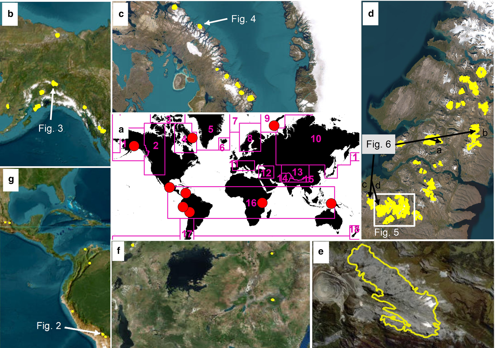
Figure 1. (a) Overview of the study regions (red dots) with RGI first order region borders in pink. Close-ups of the digitised glaciers (yellow outlines) in (b) Alaska, (c) Baffin Island, (d) Novaya Zemlya, (e) New Guinea, (f) Africa, and (g) tropical Americas. Image credits: ESRI World Imagery 2022.
Table 1. Available dates of LIA maximum extents for the investigated regions
The column ‘Close to maximum’ indicates the time, where glaciers were close to their neoglacial maximum but generally smaller than during the LIA maximum.
2.1 Alaska
In Alaska, a total of seven sub-regions across the state were selected (see Fig. 1b) to get a broader representation of the different climatic regimes. Tidewater and surge-type glaciers as well as glacier covered volcanoes are abundant in Alaska (Molnia, Reference Molnia2007). These were not included due to their different dynamic behaviour and the possible influence of volcanic activity (Barr and others, Reference Barr, Lynch, Mullan, De Siena and Spagnolo2018; Reinthaler and others, Reference Reinthaler, Paul, Granados, Rivera and Huggel2019).
Dating records show early LIA maxima in the late 15th (Brooks Range) and mid-17th (Kenai Peninsula) century (Grove, Reference Grove2004). However, most glaciers reached (or where close to) their former maximum again in the early 18th and the 19th century (Molnia, Reference Molnia2007). For the Brooks Range, even though the LIA maximum extent was reached around 1500, glaciers stayed close to this maximum until around 1890 (Evison and others, Reference Evison, Calkin and Ellis1996). For some glaciers in the Kenai Mountains (Tustemena, Bear, Pederson, Dinglestadt, Yalik, Nuka, Petrof, Exit and Grewingk glaciers) a date could be assigned to the LIA maximum glacier extent following the work of Wiles and Calkin (Reference Wiles and Calkin1994). For some of these glaciers (e.g. Grewingk, Yalik, Nuka), additional front variation changes are present going back to the first half of the 19th century (WGMS, 2021a). Information on glacier area changes since the LIA are rare for Alaska. In the Brooks Range Evison and others (Reference Evison, Calkin and Ellis1996) show an area loss of 10% between 1901 and 1981 (−0.12% a−1). The study by Molnia (Reference Molnia2007) indicates that retreat of Alaskan glaciers was constant, widespread and strong.
2.2 Baffin Island
On Baffin Island in north-east Canada (Nunavut), glaciers were mapped for several smaller sub-regions, mostly along the northern coast (see Fig. 1c). The two large inland ice caps (Barnes and Penny) were not included due to the difficulty in interpreting LIA trimlines along the entire perimeter. The main cluster of LIA extents mapped is located in the far east on the Cumberland peninsula and was partly already mapped by Svoboda and Paul (Reference Svoboda and Paul2009) using self-orthorectified ASTER images.
Way and others (Reference Way, Bell and Barrand2015) suggest a maximum LIA extent in the 17th century measured in the Torngat Mountains south of Baffin Island. Pendleton (Reference Pendleton2018) argues that glacier thinning on Baffin Island only started after 1900. Dowdeswell (Reference Dowdeswell1984) found that late neoglacial moraines stabilised on Baffin Island around 130 years ago, which would correspond to around 1854. Only limited information is available for glacier length, area or mass changes on Baffin Island for the period between the 19th century and 2000. Field measurements of length changes show a general retreat for Barnes Ice Cap (WGMS, 2021b) and a comparison to aerial photographs reveal glacier shrinkage on Bylot Island from the LIA to 1958 to 2001, with an area loss of 5% in the latter period (Dowdeswell and others, Reference Dowdeswell, Dowdeswell and Cawkwell2007). Paul and Svoboda (Reference Paul and Svoboda2009) calculated for their sample of 264 glaciers on the Cumberland Peninsula a mean relative glacier area change of −7.3% from the LIA to 1975 and of −12.5% from the LIA until 2000. Glacier mass loss accelerated after 1996 due to an increase in surface melt, exposing bare ice for a longer time and at higher elevations (Sharp and others, Reference Sharp2011; Noël and others, Reference Noël2018).
2.3 Novaya Zemlya
The third study region is located on Novaya Zemlya in the Russian Arctic (Fig. 1d), south of the Severny Ice Caps (72–74°N). In this southern part of the archipelago, glaciers do not reach the sea and are therefore well suited for LIA mapping. Nearly all suitable glaciers have been mapped in this region.
Zeeberg and others (Reference Zeeberg, Forman and Polyak2003) have shown that the maximum LIA glacier extent was reached in the second half of the 19th century, but was at a similar position before 1700. Zeeberg and Forman (Reference Zeeberg and Forman2001) suggest glaciers in northern Novaya Zemlya reached the LIA maximum already around or after 1300. Almost all glaciers displayed only one fresh moraine belt, which should correspond to the 19th century advance, while few glaciers showed two distinct moraine belts close to each other. Here, the outer one probably corresponds to early and the inner to late LIA advances. Hence, glaciers reached their LIA maximum already in the 16th century, but the re-advance in the 19th century was larger for most glaciers and destroyed related deposits.
Between the 1960s and 1990s, tidewater glaciers in the north of Novaya Zemlya stabilised due to a decrease in temperatures especially during the winter. The positive mass balance is correlated with a period of positive North Atlantic Oscillation (NAO) phase (Zeeberg and Forman, Reference Zeeberg and Forman2001). In recent decades, glaciers are continuing to retreat and in southern Novaya Zemlya they lost 3.4% of their area from ~2001 to 2016 (Rastner and others, Reference Rastner, Strozzi and Paul2017). The outlet glaciers of the large northern Ice Cap show predominantly retreat between 1992 and 2010, with a recent acceleration for tidewater glaciers (Carr and others, Reference Carr, Stokes and Vieli2014). Ciracì and others (Reference Ciracì, Velicogna and Sutterley2018) calculated a negative mass balance for the time after 2000 with a recent increase in the mass loss rate that is also confirmed in the study by Tepes and others (Reference Tepes2021).
2.4 Tropics
The region is divided into seven sub-regions across the tropics (Figs 1e–g). Five of them are located in the tropical Americas between Mexico and Bolivia, one is in Africa and one on the island of New Guinea (cf. Table S1 for details). In Mexico, LIA extents were generated for two of the three highest peaks, the Pico de Orizaba and Iztaccíhuatl. Dating records are scarce and inconclusive. Heine (Reference Heine and Lauer1975) suggests that the maximum was reached around 1850, while White (Reference White1981) mention an advance prior to 1519, and Palacios and others (Reference Palacios, Parrilla and Zamorano1999) claim the glaciers reached their maximum extent in the mid-eighteenth century but without giving further details. Existing maps from Palacios and Vazquez-Selem (Reference Palacios and Vazquez-Selem1996) and Schneider and others (Reference Schneider2008) were used as a guidance for the digitising. According to Reinthaler and others (Reference Reinthaler, Paul, Granados, Rivera and Huggel2019), glacier coverage was reduced by 71% between 1986 and 2017 with only 0.8 km2 remaining and the glacier on Popocatépetl disappeared completely after the eruption in 2000.
In Colombia, the two sub-regions were the Sierra Nevada de Santa Marta, previously studied by López-Moreno and others (Reference López-Moreno2020) and the Sierra Nevado del Cocuy, previously studied by López-Moreno and others (Reference López-Moreno2022). Dating record of moraines in the area are scarce. Van der Hammen (Reference van der Hammen, van der Hammen and Ruiz1984) dated peat samples behind the LIA moraine on Sierra Nevada de Santa Marta to 1650 while van der Hammen and others (Reference van der Hammen, Barelds, de Jong and de Veer1981) suggest that glaciers on Nevado del Cocuy were near the outer moraine in 1850. The latter is the largest ice mass of Colombia and shows an increased shrinkage since the 2000s but had a period of stagnation during the 1960s and 1970s (Rabatel and others, Reference Rabatel2013). Peaks in Ecuador were not included due to frequent volcanic activity and persistent cloud cover.
In Peru, LIA outlines for parts of the Cordillera Blanca were mapped. Jomelli and others (Reference Jomelli, Grancher, Brunstein and Solomina2008) dated LIA moraines to 1630 ± 27 years. The glacier recession already started in the 17th century and accelerated during the 19th century (Jomelli and others, Reference Jomelli, Grancher, Brunstein and Solomina2008). A re-advance occurred in the 1920s before retreating again since the 1930s and 1940s (Kinzl, Reference Kinzl1969; Rabatel and others, Reference Rabatel2013). In the first half of the 1970s glaciers stagnated or were even slightly advancing (Kaser and others, Reference Kaser, Ames and Zamora1990). Since then glaciers retreated continuously except for a short interruption during the El Niño event of 1997–1998 (Georges, Reference Georges2004).
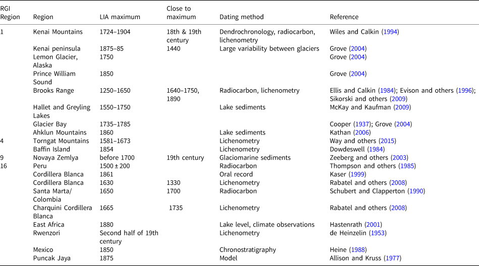
In Bolivia the focus was on the glaciers in the Cordillera Real and Cordillera Quimsa Cruz. Rabatel and others (Reference Rabatel, Machaca, Francou and Jomelli2006, Reference Rabatel, Francou, Jomelli, Naveau and Grancher2008) suggest a maximum LIA extent between 1657 and 1686, depending on the glacier. Since then, glaciers retreated steadily but experienced multiple smaller re-advances that left moraine deposits behind (see Fig. 2). Glacier recession accelerated in the late 19th century due to a drop in precipitation (Rabatel and others, Reference Rabatel, Francou, Jomelli, Naveau and Grancher2008).
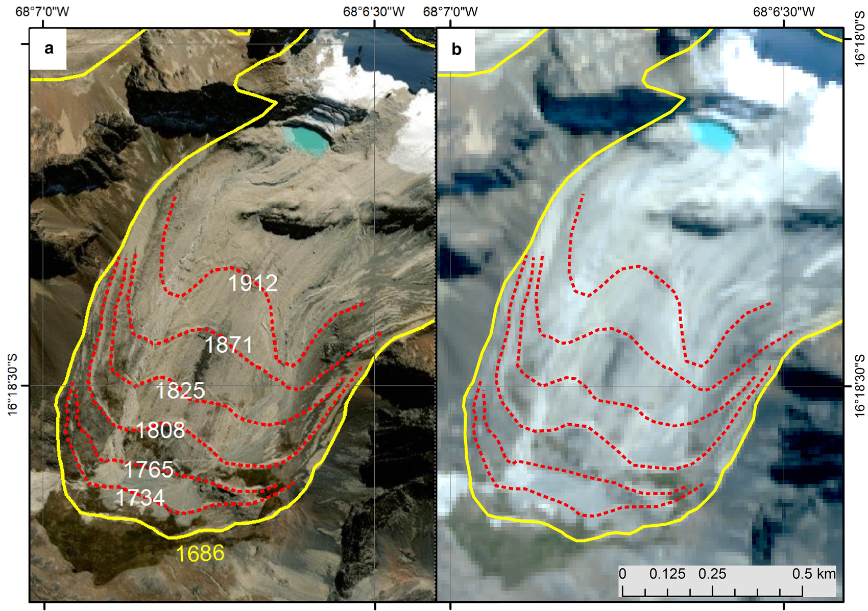
Figure 2. (a) ESRI World Imagery (Worldview 2 scene from 07.06.2019) close up of Charquini Sur Glacier in Bolivia. The panel shows the LIA maximum (yellow outline) as well as moraines from intermediate advances (red dotted) with dates taken from Rabatel and others (Reference Rabatel, Machaca, Francou and Jomelli2006). (b) Sentinel-2 natural colour composite with 10 m resolution acquired on 06.06.2019 (Copernicus Sentinel data 2019).
In Africa, glaciers were reconstructed for the three currently glacierised mountain ranges: Kilimanjaro, Mt. Kenya and the Rwenzori mountains. Dating records are scarce but Hastenrath (Reference Hastenrath2001) suggests that glacier recession started after 1880. Glaciers of the Rwenzori mountains were first mapped in 1906 by De Filippi and Kaser and Osmaston (Reference Kaser and Osmaston2002) suggest that at that time still about 90% of the glacier area was present. For Kilimanjaro, Cullen and others (Reference Cullen2013) published glacier outlines from 1912. For Mt Kenya, glaciers were first mapped in 1899 and several attempts of mapping LIA extents have been published, but none are available in a digital vector format (Hastenrath, Reference Hastenrath2005; Chen and others, Reference Chen, Wang, Guo, Wu and Wu2018). Glacier change since the LIA maximum is marked by strong recession without any known re-advances (Hastenrath, Reference Hastenrath2001). Length change measurements at Lewis glacier go back to 1893, showing a continuous retreat that has accelerated since the 1990s (WGMS, 2021a).
The LIA extent for the glaciers of Irian Jaya on the island of New Guinea in Indonesia was reconstructed. The glaciers around the highest peak Puncak Jaya could be completely mapped, and still holds a small ice mass. Allison and Kruss (Reference Allison and Kruss1977) estimated that glaciers began to retreat around 1875 and Allison and Peterson (Reference Allison, Peterson, Hope, Peterson, Radok and Allison1976) describe the retreat since then as relatively steady and uninterrupted, but small (0.3–1 m high) moraines are found within the LIA glacier limit. According to Allison and Peterson (Reference Allison, Peterson, Hope, Peterson, Radok and Allison1976) the retreat rate was especially high between 1936 and 1942 (from 13 to 9.9 km2 in six years). In 2002, only 2.25 km2 of glacier ice was left on Puncak Jaya (Klein and Kincaid, Reference Klein and Kincaid2006). The peaks Puncak Trikora, Puncak Mandala and Nagga Pilimsit also probably still had some ice cover during the LIA (Allison and Peterson, Reference Allison, Peterson, WIlliamns and Ferrigno1989). For these peaks outline generation was attempted, but due to low confidence in the resulting outlines not included in the analysis.
3. Data
3.1 WMS imagery and the ESRI world imagery
Web Map Services (WMS) providing very high-resolution images are available in a variety of formats and portals offering different applications. Some countries have opened their geo-data portals for the public (e.g. Norway, Switzerland or the US) and users can view and download geodata and view or sometimes also download the high-resolution images provided. Furthermore, it is possible to display different layers of the respective services directly in a GIS such as ESRIs ArcMap or QGIS where they can be used together with other geocoded datasets.
For this study we used the ArcMap World Imagery WMS as a main dataset for the digitising. The layer is largely based on cloud-free, very high-resolution satellite imagery with a minimum amount of seasonal snow, however, in some regions the images have clouds and seasonal snow cover. When conditions are good, the very high resolution (up to 31 cm for Worldview-3) allows a much better identification and thus more precise delineation of geomorphological features than from coarser resolution sensors such as Landsat, ASTER or Sentinel-2 (Fig. 2). When conditions are not good, the presence of snow, shadow and/or clouds can cover the trimlines and colour differences might not be visible anymore (Fig. 3). Furthermore, in some cases images are distorted in steep terrain caused by errors in the DEM used for the orthorectification.
Figure 3. (a) Example for low quality images in the ESRI World Imagery compared to (b) a Sentinel-2 infrared composite acquired on 31.07.2018 over Gakona Glacier in the Delta range, Alaska (Panel a: ESRI World Imagery; Panel b: Copernicus Sentinel data 2018).
Most scenes used in in this study originate from the commercial satellites WorldView-2, -3 and -4 as well as GeoEye1 and QuickBird 2 of Maxar Technologies (formerly DigitalGlobe). Although the acquisition date and accuracy can be extracted for individual points when using the identification tool, the borders of the stitched images are blurred and there is no possibility to visualise overlay boundaries or acquisition dates for an entire region. We have thus collected the acquisition dates and sensor names of underlying image parts (one for each glacier) manually and found that most images were taken between 2010 and 2020 (average 2016). The satellites used include Worldview-2 (67%), Worldview-3 (13%), Geoeye-1 (12%), QuickBird-2 (5%) and Worldview-4 (2%).
The given location accuracy of 5–10 m, depending on the region, is more than acceptable for LIA glacier mapping, however the frequent change of images limits the reproducibility of the data products derived from it. Also the mosaicking is sometimes imperfect and small shifts occur between neighbouring scenes. Waterman (Reference Waterman2020) provided a description on the latest update of the ESRI base map layers, but a complete changelog is not publicly available. Even though the acquisition year is not a problem for mapping geomorphological features and the mosaic is likely to only improve in the future, the meta information should get better access.
3.2 Modern outlines
Modern glacier outlines in shapefile format were used as a starting point for the LIA outline digitising and as a reference for the modern extent (see Table 2). After visual inspection of the outlines in RGIv6, we decided to use recently revised or newly created outlines for Bolivia, Baffin Island, Novaya Zemlya and Rwenzori referring to the years 1998, 2000, 2016 and 2021, respectively. For Peru, the freely available outlines from the national inventory from 2016 were chosen as a starting point. For Alaska and the other tropical regions (Colombia, Mexico, parts of Africa and New Guinea) the RGIv6 outlines from around the year 2000 were selected. However, we selected glaciers where the outline does not include wrongly mapped snow patches or shows a generalised delineation.
Table 2. Overview of the input datasets used and their characteristics
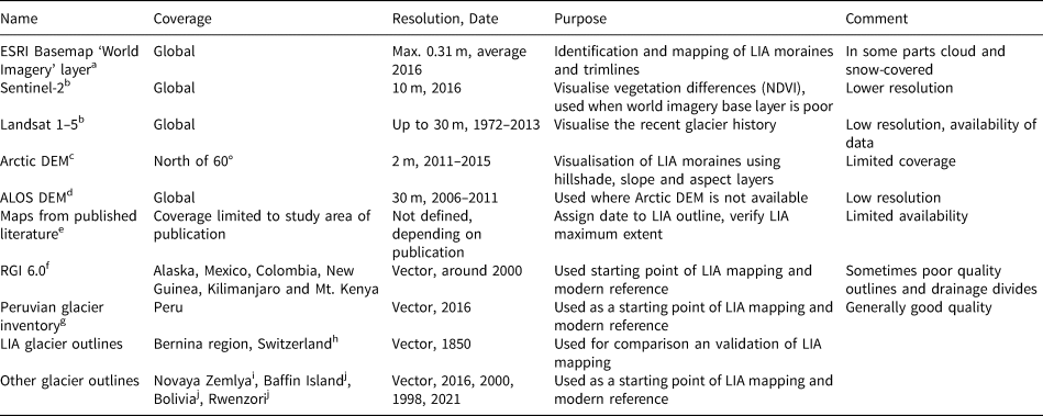
a Source depending on the region. See World Imagery: https://www.arcgis.com/home/item.html?id=10df2279f9684e4a9f6a7f08febac2a9.
e Maps from Allison and Peterson, Reference Allison, Peterson, WIlliamns and Ferrigno1989; Wiles and Calkin, Reference Wiles and Calkin1994; Palacios and Vazquez-Selem, Reference Palacios and Vazquez-Selem1996; Kaser and Osmaston, Reference Kaser and Osmaston2002; Hastenrath, Reference Hastenrath2005; Rabatel and others, Reference Rabatel, Machaca, Francou and Jomelli2006, Reference Rabatel, Francou, Jomelli, Naveau and Grancher2008; Schneider and others, Reference Schneider2008; López-Moreno and others, Reference López-Moreno2020.
g http://catalogo.geoidep.gob.pe:8080/metadata/srv/api/records/1099ce9e-bd97-49c1-a32a-2eccb35fcf79.
i Rastner and others (Reference Rastner, Strozzi and Paul2017).
j unpublished.
3.3 Coarser-scale and nonoptical imagery
Where the ESRI world imagery layer displayed snow, clouds or errors from shifts or stiches, false colour infrared images (bands 8, 4, 3 as RGB) with 10 m resolution from Sentinel-2 were used. With the inclusion of the near infrared band, differences in vegetation cover along the trimlines are very distinct and aid in the interpretation (see Fig. 3). In order to facilitate the visual interpretation and confirm the observed trend of glacier retreat, occasionally also early Landsat 1–5 images were analysed. They revealed a rough indication of the 30 to 40-year retreat for the related glaciers and allowed us to estimate if the mapped LIA extent is reasonable. Elevation data (ArcticDEM, Version 3 and ALOS Global Digital Surface Model (AW3D30), Version 3.1) were used to extract contour lines as well as hillshade and aspect layers. These are useful to visualise the topography and identify the crest of a moraine ridge, where the LIA glacier margin is thought to have been (Bennett, Reference Bennett2001; Glasser and Jansson, Reference Glasser and Jansson2008; Hein and others, Reference Hein2010). The Arctic DEM hillshade and aspect layers were loaded into the GIS environment through the ArcGIS online WMS. This allowed us to preserve the full 2 m resolution without downloading the raw data. Due to its high spatial resolution, the ArcticDEM continues to be a reliable tool in mapping glacio-geomorphological landforms (Levy and others, Reference Levy2017; Chandler and others, Reference Chandler2018). Finally, published maps and photographs which show the former glacier extents and moraine locations were considered (for details see Table 2).
4. Methods
4.1 Selection of suitable (sub-)regions
Within an RGI region, suitable subregions were selected for LIA mapping according to the following criteria:
(1) No or a limited number of LIA glacier outlines available in the GLIMS database
(2) Dating records available (not for RGI regions 4 and 9)
(3) High quality of modern outlines (visual inspection of available products)
(4) High-resolution ESRI world imagery available (at best no clouds or shifts)
(5) Moraines and trimlines generally visible
(6) No (or only few) calving glaciers at LIA extent
After a review of existing publications with LIA outlines and searching within the GLIMS glacier database, RGI regions with existing digitally available LIA outlines were excluded. In the GLIMS database, LIA outlines are currently only available for southern Patagonia (Davies and Glasser, Reference Davies and Glasser2012) and the Alps (Maisch and others, Reference Maisch, Wipf, Denneler, Battaglia and Benz2000; Fischer and others, Reference Fischer, Seiser, Stocker Waldhuber, Mitterer and Abermann2015). For Alaska, Sikorski and others (Reference Sikorski, Kaufman, Manley and Nolan2009) and Wiles and Calkin (Reference Wiles and Calkin1994) mapped LIA extents for the Brook Range and Kenai Peninsula, respectively, but digital outlines were not available. For Baffin Island, the previously mapped LIA outlines by Paul and Kääb (Reference Paul and Kääb2005) or Paul and Svoboda (Reference Svoboda and Paul2009) could not be used due to geolocation (different DEMs were used for orthorectification) and topologic issues (preliminary or different ice divides). For the tropics, maps with LIA glacier outlines were available in published papers, but no digital outlines (Allison and Kruss, Reference Allison and Kruss1977; Allison and Peterson, Reference Allison, Peterson, WIlliamns and Ferrigno1989; Hastenrath, Reference Hastenrath2005; Rabatel and others, Reference Rabatel, Machaca, Francou and Jomelli2006, Reference Rabatel, Francou, Jomelli, Naveau and Grancher2008; Schneider and others, Reference Schneider2008). Nothing was available for the study region in Arctic Russia. Studies that provided glacier-specific dating records and sketches of glacier outlines were prioritised when selecting the subregions.
The selected subregion should ideally consist of a cluster of glaciers (or small mountain range) with glaciers in different size classes, aspects and geometries. If possible, different subregions should cover a variety of climate regimes within an RGI region. For example, coastal as well as inland sub-regions were selected for Alaska. Within a sub-region, the goal was to map as many glaciers as possible with a sufficient quality. Calving glaciers and glaciers with limited visibility of trimlines were excluded. We have also excluded very large glaciers (larger than a hundred km2) since glaciers in these size classes are not present in all regions, making related change rates difficult to compare. Additionally, the response time of such large ice masses might be larger than our observation period. To have a representative sample size, each sub-region should consist of at least ten glaciers (when possible) with a total number of about 100 glaciers per RGI region. For full details about the sample size and location of each sub-region see Table S1 in the Supplementary Material.
4.2 LIA mapping workflow
After selecting the sub-regions, suitable imagery, modern glacier outlines and elevation data were collected for each specific sub-region. LIA glacier outlines were created by modifying the modern outlines within the ArcMap software. The outline was digitised manually along the trimlines and crests of terminal moraines as visible in the ‘World imagery’ layer and similar to the studies by Carrivick and others (Reference Carrivick2019) and Lee and others (Reference Lee2021). Gaps in the trimlines were manually interpolated. The delineation of the LIA outline in the ablation area was the main focus of the digitising. Changes in the accumulation area were only considered when clear trimlines were visible, indicating significant surface lowering. With the very high-resolution images, it is possible to visualise them on a small scale (around 1: 10 000), identify small moraines and differentiate the moraine ridge from its foot, which might not be possible with coarser resolution (>5 m) images. As Smith and Clark (Reference Smith and Clark2005) also suggested, using multiple data sources results in a better and more complete visualisation of the features to be mapped. We have thus considered the following additional information layers.
For the Arctic regions, a comparison to the ArcticDEM (hillshade, aspect map) added certainty to the interpretation of the moraines and verified the position of the crests. Whereas the interpretation of single crested moraines is straightforward, uncertainties remain for multi-crested moraines (Bennett, Reference Bennett2001). In such a case, the highest crest of the moraine was chosen. In the case more than one moraine belt is present within the range of typical LIA variability (cf. Fig. 2a), the outermost, often most complete and best visible one was digitised, assuming it to represent the LIA maximum extent. Possible outer moraine fragments indicating a larger extent have not been considered for digitising. Our approach is thus different to Carrivick and others (Reference Carrivick, James, Grimes, Sutherland and Lorrey2020), who used a more conservative approach and mapped the innermost moraine belt which could relate to a later advance but not necessarily the LIA maximum extent.
The general position of the trimlines was chosen according to the colour difference in the Sentinel-2 images, back-checked and refined with the ESRI world imagery layer. For the glaciers in Africa and New Guinea the geomorphological evidence of former glacier extents was very limited. For these regions we scanned, digitised and geocoded the dated glacier outlines as published in the literature (Allison and Kruss, Reference Allison and Kruss1977; Allison and Peterson, Reference Allison, Peterson, WIlliamns and Ferrigno1989; Kaser and Osmaston, Reference Kaser and Osmaston2002; Grove, Reference Grove2004; Hastenrath, Reference Hastenrath2005).
Calving glaciers were excluded due to the low confidence of reconstructing the part that is possibly under water. Using bathymetry data like Dowdeswell and others (Reference Dowdeswell, Ottesen and Bellec2020) is a method to map LIA extents of tide-water glaciers, but was not applied here.
4.3 Uncertainty assessment
4.3.1 Reproduction and interpretation uncertainty
The uncertainty assessment of the geomorphological mapping is divided into two main contributors: the reproduction or digitising uncertainty (r) and the interpretation uncertainty (i). The former describes the uncertainty introduced by imprecise digitising (e.g. outlines will be at different positions when digitised independently twice or more) and the latter can be related to the interpretation of geomorphological features by the analysts, introduced for example by manually bridging gaps in the trimlines or interpretation of moraine complexes. Although r will increase with i, we treat both uncertainties as independent as we have determined r for a fixed dataset. The resulting total uncertainty (σ) for a single LIA outline is thus:
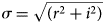
For (r), 18 glaciers from all three quality classes (see 4.3.2) and size classes were digitised six times (Figs 4a–c). Nine glaciers on Baffin Island and nine in Alaska, resulting in a total of 108 outlines for each region, three large, medium and small glaciers were selected, one per quality class. To quantify the reproduction uncertainty the standard deviation (s.d.) of the resulting mean glacier area differences was calculated. Another way to measure the differences of multiple digitisations is an overlap count (Fig. 4d). For this, the largest (one overlap) possible and smallest possible (6 overlaps) area of all digitised areas was calculated. To get a better insight on the advantages of using very high-resolution images for the mapping, a further multiple digitising experiment was performed for the same 18 glaciers using 10 m Sentinel-2 composites and only three rounds of digitisations.
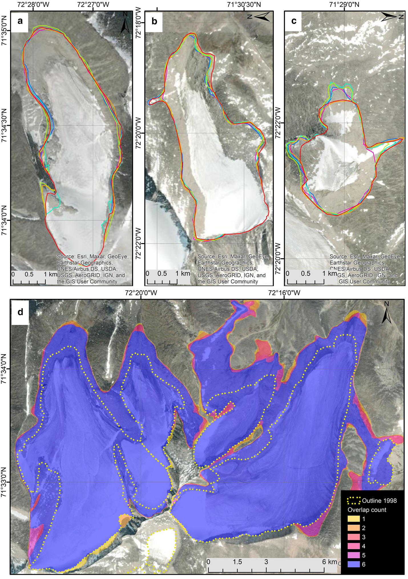
Figure 4. (a–c) Visualisation of the multiple digitisation experiment for three glaciers on Baffin Island. (d) Colour-coded multiple digitising overlap count for two glaciers on Baffin Island. All background images: ESRI World Imagery 2022.
In order to quantify (i), a cluster of 17 glaciers on Novaya Zemlya were digitised independently by the two authors with the same input dataset (Fig. 5). Both have experience in glacio-geomorphological landform interpretation from satellite images and can thus be seen as expert analysts. To get a value for (i) we used the s.d. of the relative differences to the mean area.
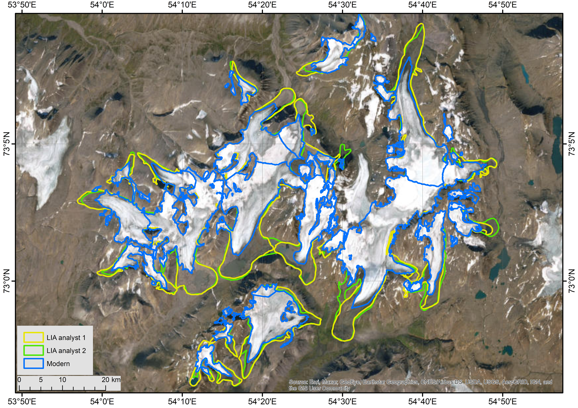
Figure 5. Overlay of glacier outlines from the interpretation experiment with two analysts for 18 glaciers in Novaya Zemlya. Background image: ESRI World Imagery, 2022.
Secondly, nine glaciers in Bolivia that were already digitised (but not digitally available) by Rabatel and others, (Reference Rabatel, Machaca, Francou and Jomelli2006, Reference Rabatel, Francou, Jomelli, Naveau and Grancher2008) were compared with the new and independently created outlines from this study. To this end, area values for the glaciers of Charquini, Huayna Potosi, Jankhu Uyu and Wila Lluxita, Zongo and Tarija were compared and the relative difference as well as the s.d. calculated. Thirdly, the LIA extents of 25 glaciers in the Bernina region of Switzerland were digitised independently and results compared to outlines derived by Maisch and others (Reference Maisch, Wipf, Denneler, Battaglia and Benz2000) from cartographic interpretation of historical maps, aerial imagery and geomorphological evidence from field observation.
Generally, the geolocation uncertainty of the input data (e.g. shifts of the ‘World imagery’ layer) has to be kept in mind as a further source of uncertainty. It has, however, not been further investigated.
4.3.2 Quality classification
Independent, but related to i, we introduced for each glacier a simplified quality classification to subjectively quantify the visibility of the geomorphological features (moraines and trimlines) and thus the resulting outlines. It was developed based on first experiences in region 3 (Novaya Zemlya). The scale ranges from 1 to 4 and examples are illustrated in Figure 6:
(1) Unusable, meaning that without major visual interpolation between parts of moraines or trimlines it is not possible to generate a complete outline with sufficient quality. This applies also to small glaciers that did not leave any moraines or trimlines. Outlines with a quality of 1 were not included in the analysis.
(2) Usable, some parts of the moraine are not visible but in general the former shape of the glacier is well represented. Modern outlines or satellite images with a small geographical shift also fall into this category.
(3) A good outline where most of the moraine and trimline are well visible.
(4) A very good outline with only minor uncertainties or interruptions (e.g. where the glacier river is cutting through a terminal moraine).
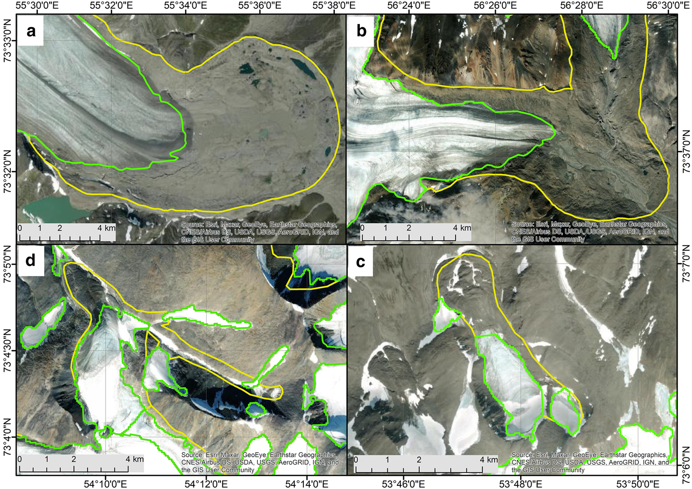
Figure 6. Four panels showing examples for the assigned quality classes. These are (clock-wise): (a) very good (class 4) showing a near perfect moraine belt and trimline. (b) Good (3) showing a well-defined trimline, only parts of the front moraine were eroded and some cloud cover on the southern side. (c) Usable (2) showing a multi-crested front moraine but trimlines are less clear. (d) Unusable (1) showing an example where probably snow was mapped as a glacier in the modern outlines and no clear trimlines are visible. All background images: ESRI World Imagery layer, 2022.
The quality classification is a subjective interpretation of the confidence regarding the LIA outline. It could vary with the analyst and is thus only a tool for categorising the resulting sample rather than a strict statistical uncertainty calculation.
4.4 Selection of LIA maximum dates for each region
Glaciers did not reach their LIA maximum extents coherent and synchronous across the globe (Rabatel and others, Reference Rabatel, Francou, Jomelli, Naveau and Grancher2008; Schaefer and others, Reference Schaefer2009). In Table 1 the related dating records relevant for this study are listed, further details can be found in Table S2 of the Suppplementary Material.
Overall, the records show the following trends:
(1) Glaciers in high latitudes started retreating only in the second half of the 19th century, but earlier advances had a similar (yet mostly smaller) magnitude.
(2) Glaciers in Mexico, Africa and New Guinea also reached their LIA maximum in the mid or end of the 19th century.
(3) Glaciers in the tropical Andes reached their maximum earlier (17th century) and have been retreating since then (often with several minor readvances creating moraine walls).
As each glacier has a different response time, the time at which the maximum extent was reached also varies. Hence, the use of generalised dates for the entire region works better for regional change assessment than for individual glaciers. For the trends described under point (1), we selected the date of retreat instead of moraine deposition, as the glaciers in these regions might have been stationary for several decades with resulting smaller change rates if not considered. Carrivick and others (Reference Carrivick, James, Grimes, Sutherland and Lorrey2020) showed that glacier volume change rates tripled when changing the maximum extent from the year 1450 to 1800. Choosing a fixed year, for example 1850, for all studied glaciers would provide consistent change rates, in particular as most of the glacier change happened since the 20th century. This is only questionable for tropical regions. In Bolivia for example, glaciers already lost 20% of their area by the middle of the 19th century (Rabatel and others, Reference Rabatel, Francou, Jomelli, Naveau and Grancher2008). Therefore, for the regions of Colombia and Bolivia, 1650 was chosen as the starting point and 1630 for Peru (Schubert and Clapperton, Reference Schubert and Clapperton1990; Jomelli and others, Reference Jomelli, Favier, Rabatel and Brunstein2009). For the Brooks Range the selected LIA maximum date is 1890 (Evison and others, Reference Evison, Calkin and Ellis1996), even though glaciers were slightly larger between 1250 and 1650 (Sikorski and others, Reference Sikorski, Kaufman, Manley and Nolan2009) and for the Ahklun Mountains it is 1860 (Kathan, Reference Kathan2006). For New Guinea, 1875 (Allison and Kruss, Reference Allison and Kruss1977) was chosen as a starting point and for Africa 1880 (Hastenrath, Reference Hastenrath2001). Additionally, due to poorly visible moraines and trimlines, for Mt. Baker in Rwenzori and Kolbe glacier on Mt Kenya, stages were taken from 1906 (Kaser and Osmaston, Reference Kaser and Osmaston2002) and 1899 (Hastenrath, Reference Hastenrath2005) respectively. As these extents do not refer to the LIA maximum, the areas were considered to be 90% of the maximum extent, as suggested by Kaser and Osmaston (Reference Kaser and Osmaston2002). For glacier without any precise dates like Baffin Island, Novaya Zemlya and parts of Alaska, 1850 was selected.
In order to incorporate uncertainties into the area change rate calculations, lower and upper bounds were also calculated. Dating of LIA moraines is often based on lichenometry, which can have large uncertainties due to the lack of standardised measurement methods and variations in lichen growth rates (Osborn and others, Reference Osborn, McCarthy, LaBrie and Burke2015; Armstrong, Reference Armstrong2016; Emmer and others, Reference Emmer, Juřicová and Veettil2019). Rabatel and others (Reference Rabatel, Francou, Jomelli, Naveau and Grancher2008) give uncertainty values for the dating with lichenometry of around ± 25 years. As we do not have glacier specific dating records for all regions but rather estimations from literature and response times among glaciers might differ, the uncertainties are likely larger. Therefore, we calculated change rates with a lower and upper bound of ±50 years from the mean value of a region.
4.5 Area changes and topographic information
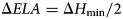
Prior to the area change assessment, modern ice bodies that previously formed one larger LIA glacier were merged to allow for a direct comparison. For these merged glaciers as well as the LIA glaciers, the area and a set of topographic parameters were calculated. The area was calculated using a cylindrical equal area projection within ArcMap. As topographic parameters, maximum minimum and mean elevations were extracted from the corresponding modern DEM as well as mean slope and aspect. Calculating the mean elevation change is not reliably possible without considering glacier thinning and the LIA glacier surface. However, changes in ELA can be estimated following Haeberli and Hoelzle (Reference Haeberli and Hoelzle1995) by Eqn (2), assuming the maximum elevation did not change. It is further assumed here that the ELA is the balanced budget ELA0, which can be approximated by the midpoint elevation of a glacier (Raper and Braithwaite, Reference Raper and Braithwaite2009).
5. Results
5.1 New LIA glacier outlines for four regions
In total, we digitised LIA outlines for 493 glaciers covering an area of 4640 km2, of which 152 glaciers (2449.3 km2) are in Alaska, 126 (1198.4 km2) on Baffin Island, 85 (644.0 km2) on Novaya Zemlya and 126 (338 km2) in the tropics. Comparing this with the total glacier area of the respective RGI region, this is a coverage of roughly 2.3% (RGI_01), 2.5% (RGI_04), 0.9% (RGI_09) and 5.7% (RGI_16) (RGI Consortium, 2017). Although the percentages seem to be very small, the glaciers selected represent the size-class distribution rather well and are better indicators of climate change than for example the large ice caps on Baffin Island or the huge and often complex glacier systems in Alaska. The glacier distribution per size class and the four main regions is presented in Figure 7. Although glaciers in different size classes were selected for each region, differences between the regions remain. For example, the sample of tropical ice masses lacks glaciers larger than 25 km2 and 60% of them are smaller than 2 km2. Glaciers that have split since the LIA changed the glacier count from 493 LIA glaciers to 891 ice bodies in the modern inventories (271 in Alaska, 206 on Baffin Island, 172 on Novaya Zemlya and 242 in the Tropics) and a further 25 melted completely.
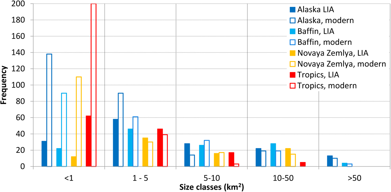
Figure 7. Frequency histogram of the size classes per region for both LIA and modern glaciers. Note that the glacier breakup for the modern glacier was included here, hence overall more modern glaciers are counted. Disappeared glaciers are in the size class <1 km2.
5.2 Area changes
The total glacier area of 4640 km2 during the LIA shrunk to about 3590 km2 (−22.6%) in modern times. Total and relative regional glacier area changes are −1023.6 km2 (−20.0%) for Alaska, −490.3 km2 (−15.2%) for Baffin Island, −168.7 km2 (−26.2%) for Novaya Zemlya and −205.3 km2 (−60.8%) for the tropics (Table 3 and Fig. 8). For the tropical regions, the largest shrinkage was observed in Mexico (−89%), Africa (−87%) and Puncak Jaya on New Guinea (−90%). Shrinkage was smaller in Colombia (−68%) and in Peru and Bolivia (−46%). In Alaska, the sub-region with the largest change is the Talkeetna Mountains, which lost 34% of their LIA area. The smallest change was observed in the Kenai Mountains on the southern coast. Here, the glaciers lost just 10% of their area since the LIA maximum extent and for example, the comparably large (316.1 km2) Tustumena Glacier lost just 2.7% since its maximum position.
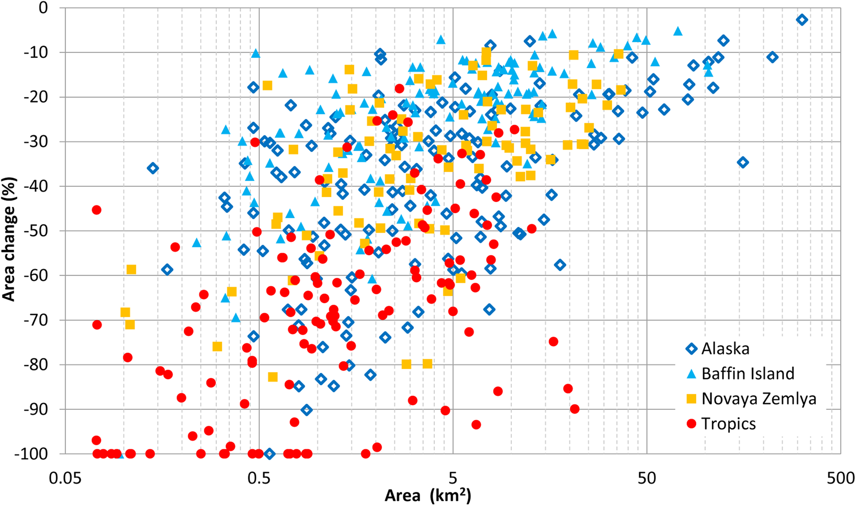
Figure 8. Relative area change vs LIA area for individual glaciers. The four main regions are colour-coded, effects of the different LIA timing are not considered.
Table 3. Overview of the mapping and area change results as well as changes in minimum elevation (‘±’ indicates one standard deviation)
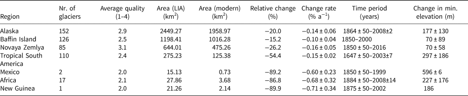
Quality classification from 1 (worst) to 4 (best), see chapter 4.3.2.
As the total area changes are impacted by glacier size (Fig. 8), we have also calculated a mean change from the individual relative change values, i.e. not normalised by area. In Alaska, the mean relative area loss when normalised by area for the 152 glaciers is −39 ± 20% since the LIA, for Baffin Island it is −25 ± 15%, on Novaya Zemlya −35 ± 17% and in the tropics −68 ± 22%. Larger glaciers lost generally relatively less area compared to smaller ice bodies. Hence, higher values in the normalised area change compared to the averaged total relative change indicate that the latter is dominated by large glaciers with small relative change, but large absolute change. This is the case for all four main regions, but in the tropics the difference is smaller, as the region is dominated by smaller glaciers (see Fig. 7) and also many of the larger glaciers in the region lost relatively large amounts of area (Fig. 8).
The scatterplot (Fig. 8) reveals that most glaciers have sizes between 0.5 and 15 km2. In all regions the scatter of change values and the relative area loss increases towards smaller glaciers. The tropics show the most severe glacier loss with more than 80% of the glaciers having lost more than half of their area and many of them melted away completely (−100%). Also, five glaciers larger than 5 km2 show area losses exceeding 70% whereas in the other three regions most values in this size range lost between 10 and 40%. The individual changes in the three Arctic regions are rather similar, but for the same size classes it appears that glaciers on Baffin Island had the smallest area loss, Novaya Zemlya a greater loss and Alaska the greatest loss. All relative change values per size class are listed in Table 4.
Table 4. Count and area changes per size class
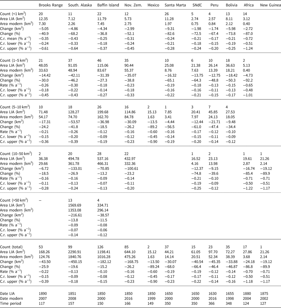
Columns are the subregions (SNdC, Sierra Nevado del Cocouy; Nov. Zem., Novaya Zemlya) and rows list glacier count, areas and changes for each size class, which is given in the first row of each section (after ‘Count’). LIA dates are averages for all size classes. Mean area change rates (C.r.) with lower (+50 years) and upper (−50 years) bounds of the time period.
5.3 Area change rates
5.3.1 Regional values and impact of LIA date
Glacier area change rates were calculated using the LIA dates listed in Section 4.4 and Tables 3 and 4, yielding −0.10% a−1 for Baffin Island, −0.14% a−1 for Alaska, −0.16% a−1 for Novaya Zemlya, −0.15% a−1 for tropical South America and −0.68% a−1 for the remaining tropical glaciers. If we split the Alaskan main range into smaller parts, change rates are lowest on the Kenai peninsula with −0.07% a−1 between 1851 and 2005 followed by the South Boundary Ranges with −0.12% a−1 (1850–2007). Highest rates were observed in the Brooks Range (1890–2002), Ahklun (1860–2009) and Talkeetna Mountains (1850–2009) with −0.22% a−1 within their respective time period. Glaciers in Mexico (−0.60% a−1), Africa (−0.68% a−1) and New Guinea (−0.71% a−1) show a much higher area loss rate compared to the South American glaciers. This can be due to the much earlier LIA date of the latter (around 1650 instead of 1850 or 1880), but values remain higher even when considering a 17th century starting point. This is due to the fact that they lost nearly 90% of their LIA area. The different slopes of the lines in Figure 9a show the impact of the LIA timing on the calculated change rates. Compared to the three Arctic regions with about the same LIA date, the area loss rates in Mexico, Africa and New Guinea are about five times higher.
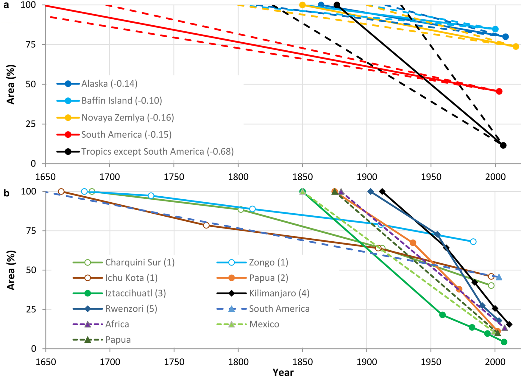
Figure 9. Relative glacier changes for (a) all regions (numbers in brackets are change rates (% a−1), dashed lines are the changes for ±50 years uncertainty) and (b) tropical regions with additional values from the literature: (1) Rabatel and others (Reference Rabatel, Francou, Jomelli, Naveau and Grancher2008); (2) Allison and Peterson (Reference Allison, Peterson, Hope, Peterson, Radok and Allison1976), Klein and Kincaid (Reference Klein and Kincaid2006); (3) Schneider and others (Reference Schneider2008); (4) Cullen and others (Reference Cullen2013); (5) Kaser and Osmaston (Reference Kaser and Osmaston2002), Taylor and others (Reference Taylor2006). Dashed lines are results from this study, dates are regional averages.
In Figure 9b we compare the values of our post-LIA time frame with data including intermediate steps from the literature. These additional values are in good agreement to the long-term trend from this study. All selected glaciers express a near constant retreat since the LIA maximum with only minor fluctuations. An example for differentiating trends is found on Iztaccíhuatl, where the change rate decreased after 1959 from −0.72 to −0.36% a−1 (Schneider and others, Reference Schneider2008) whereas on Puncak Jaya it increased after 1936 from −0.54 to −0.85% a−1 (Allison and Peterson, Reference Allison, Peterson, Hope, Peterson, Radok and Allison1976, Reference Allison, Peterson, WIlliamns and Ferrigno1989; Klein and Kincaid, Reference Klein and Kincaid2006).
A ±50 years difference in the change rate calculation (between lower and upper bound) has a high impact on shorter time periods like for the Arctic regions and the tropics outside of South America. The relative difference between lower and upper bound varies in the Arctic regions for Novaya Zemlya from −0.12 to −0.23% a−1 and for Brooks Range from −0.15 to −0.39% a−1. It has a lesser impact on the much longer time periods in South America, where the rates only change from −0.13 to −0.18% a−1 when the LIA maximum date is assumed to be 50-years later or earlier, respectively.
5.3.2 Change rates per size class
Due to the dependence of relative area change on glacier area (the dependence is even stronger for absolute area changes), in Table 4 we compare mean area changes per size class across individual sub-regions. Apart from the fact that not all size classes are populated across all regions (c.f. also Fig. 7), differences across regions in a specific size class are much better comparable, i.e. revealing climate change rather than glacier size impacts.
In general, change rates decrease with increasing glacier size across all regions, which is also obvious from the scatter plot in Figure 8. Shrinkage rates are consistently highest in Mexico, New Guinea and Africa. For the other tropical sub-regions in South America, change rates are lowest in Peru for glaciers smaller than 5 km2 and in Bolivia for glaciers between 5 and 10 km2. Colombian glaciers (regions Santa Marta and Sierra Nevada del Cocouy) generally have the highest area loss rates of the analysed South American glaciers. For the Arctic regions, apart from the change rate itself, also the difference in change rates between the regions decreases with increasing glaciers size. Glaciers in southern Alaska show the highest shrinkage rate of all Arctic regions across all size classes, but the differences are small. Interestingly, the change rates for glaciers <10 km2 are higher in the Arctic than in the four tropical regions of South America. At first glance, this is due to the more than two times longer time period (approx. 150 vs. 350 years) used for averaging. Over a similar time period the change rates would be more similar. However, glaciers in tropical South America were often already much smaller in 1850 compared to their 1650 LIA maximum extents (Figs 2 and 9b), implying that for smaller glaciers the change rates in Arctic regions are indeed higher than in tropical South America. Also, when considering the lower and upper bounds of the change rates, this trend is less clear. The lower bound values for glaciers smaller than 10 km2 in the Arctic regions (−0.09 to −0.33% a−1) are similar to the upper bound values in tropical South America (−0.12 to −0.28% a−1). In general, the influence of glacier size on the sensitivity of timing to change rates is less visible as it is about constant across all size classes.
5.4 Topographic changes
The analysis of the topographic changes presented in Table 3 reveal that the largest changes are observed again in the tropics with an average minimum elevation (H min) rise of 302 ± 186 m, followed by Alaska with 177 ± 130 m. Baffin Island and Novaya Zemlya show similar changes with 70 ± 89 m and 70 ± 58 m, respectively (the ± indicates one standard deviation). This would result in approximated ELA0 changes of 151 m for the tropics, 88.5 m for Alaska and 35 m for Baffin Island and Novaya Zemlya.
5.5 Uncertainty estimation
5.5.1 Input data accuracy
The ESRI ‘World imagery’ layer has a horizontal geolocation accuracy of 5–10 m depending on the region (according to the layer attribute data). In some places, shifts and distortions are easily identifiable, for example in steep parts on Mt. Kenya. Generally, the ‘World imagery’ layer compares well with Sentinel-2 images with in most cases no shifts visible by eye. The lateral accuracy of Sentinel-2 images is according to Kääb and others (Reference Kääb2016) around 10 m or less. For Landsat 8, a horizontal shift towards Sentinel-2 was observed in isolated cases (30–50 m). This is mostly due to the different DEMs used for the orthorectification of the images (Kääb and others, Reference Kääb2016).
5.5.2 Reproduction uncertainty
The results of the reproduction or digitising uncertainty experiment show a mean relative difference to the average area of 1.4% with a s.d. of 1.3% (Fig. 10). Generally, small glaciers (<10 km2) show a slightly higher mean difference of 1.6% compared to large glaciers (>10 km2) with 1.0%. The influence of the subjective quality scale on the reproduction uncertainty is less clear than expected. Whereas the quality class 4 showed indeed the smallest mean difference (1.2%) classes 2 and 3 showed very similar values (1.4 and 1.5%, respectively).
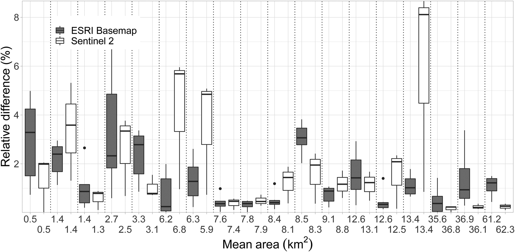
Figure 10. Relative area differences of outlines generated by multiple digitising using the ESRI World Imagery (grey boxes) vs Sentinel-2 (white). Each pair represents the same glacier with mean area values for both approaches on the x-axis. The horizontal lines in the box plots represent the median, boxes the inter-quartile range, lines the minimum and maximum and points outliers.
Regarding the overlap count, the average difference between one and six overlaps is 10.6% with a standard deviation of 5.3%. This would give an error margin of ±5.3%. There is a correlation with the glacier size with small (<10 km2) glaciers showing a higher average difference of 12.0% with a s.d. of 5.8% whereas larger glaciers (>10 km2) only show 7.9% with a s.d. of 3.1%. With differences being generally small (half of the reproduction uncertainty resulted in a difference of less than 1%), the correct interpretation of moraine features plays a more important role than the reproduction ability. As shown in Figure 4a for the case of a clearly visible trimline, differences between digitisations are minimal (10–40 m), but with different interpretations (Fig. 4c) the resulting differences are much larger.
5.5.3 Interpretation uncertainty
The results of the interpretation experiment show that, on average, the difference between the two analysts was 1.9% with a standard deviation of 10%. Front moraine positions had generally a good agreement, most differences arise from interpreting side branches of the glacier as well as when push moraines with multiple crests are found (Fig. 5). The resulting area was with 186.0 and 185.3 km2 almost identical, meaning that different interpretations cancel each other out for a large enough dataset if the expertise of moraine and trimline interpretation is similar.
Comparing the results of the nine glaciers digitised by Rabatel and others (Reference Rabatel, Machaca, Francou and Jomelli2006, Reference Rabatel, Francou, Jomelli, Naveau and Grancher2008) with this study, the total areas are 18.10 and 17.56 km2 respectively, i.e. just 3% smaller. The average difference is 3.9% with a standard deviation of 14.7% and therefore slightly larger compared to the experiment on Novaya Zemlya. The higher differences can be related to different input data such as satellite images and resolution, reference outlines and drainage divides.
Lastly, LIA outlines of 25 glacier in the Bernina region of Switzerland (Fig. S1) were compared with outlines generated by Maisch and others (Reference Maisch, Wipf, Denneler, Battaglia and Benz2000) yielding total areas of 72.98 and 71.27 km2, respectively. The average relative difference was 8.4% with a standard deviation of 13.7%. The former is slightly larger than for the experiments in Novaya Zemlya and Bolivia, but the spread falls between the two. The largest differences result in different interpretations of frontal position as well as complex moraine deposits (e.g. extended ice-cored lateral moraines). Interestingly, 18 out of 25 glaciers were digitised with a smaller area compared to the reference dataset. This is partly due to a conservative mapping approach, especially in the accumulation area and whether or not the geomorphological features are visible and how fast vegetation recovery is. When only the lower parts of LIA extents are digitised and trimlines are well visible, the uncertainties would be smaller. Overall, the mean relative difference is much larger for small glaciers, but total areas agree well as this value is dominated by large glaciers with a smaller uncertainty.
5.5.4 Comparison with Sentinel-2
In order to quantify the added value of using very high-resolution images for LIA glacier mapping, the same glaciers as used in Section 5.5.2 were independently digitised using 10 m Sentinel-2 scenes. Each glacier was digitised three times, each one on separate days without viewing the previous digitising. The comparison reveals a mean relative difference to the average area of 1.7% with a s.d. of 2.0% and is thus slightly higher than with the ‘World imagery’ layer. As shown in Fig. 10, the uncertainty decreases somewhat towards larger glaciers and Sentinel-2 uncertainties are sometimes but not in general higher. For ten of the eighteen glaciers, Sentinel-2 derived areas are (when normalised by area) on average 1.6% smaller but without a dependence on glacier area. Also, a direct correlation of the mean difference to the subjective quality classification did not emerge. We assume that a larger sample size would be needed to detect such a correlation. In conclusion, images with 10 m spatial resolution also allow mapping of LIA outlines with a sufficient quality. What might not be possible is the correct interpretation of small-scale geomorphologic features like multi-crested moraines or moraines from intermittent advances.
5.5.5 Quality classification
As a second step to estimate the uncertainty, the subjective quality scale described in Section 4.3.2 was helpful. Glacier extents with a low-quality assignment should have a higher uncertainty. However, for the sample discussed in Section 5.5.2 results are inconclusive. The quality level should thus be seen as a subjective measure of the difficulties in interpretation and digitising rather than a value suitable for calculation. The average quality for each region is listed in Table 3. Best LIA mapping conditions were found in Novaya Zemlya with an average quality score of 3.1. This means overall, moraine and trimline visibility was superior compared to other regions. Also, vegetation recovery is slower in Arctic regions resulting in a somewhat higher mean score. In tropical regions the quality scores are lower (2.4), as steep slopes, bedrock and generally small glaciers are harder to digitise.
5.5.6 Total uncertainty
The total mapping uncertainty consists of the standard deviation of the interpretation and reproduction uncertainty and is calculated following Eqn (1). The result is 10.1%. This leads to a total LIA area of 4640 ± 232 km2. Due to the limited mapping in the accumulation area this is a lower bound LIA area estimate. Reproduction uncertainty (1.3%) can be considered as a minor contributor to the total uncertainty. More important is the interpretation uncertainty (10%), where the ability of the analyst to correctly identify and interpret moraine features is more important than for example image resolution. Higher resolution images help with the identification and allow a larger ground sampling distance. This was also found by Chandler and others (Reference Chandler2018).
6. Discussion
6.1 Potential and shortcomings of the world imagery layer for LIA mapping
The use of a WMS like the ESRI world imagery layer or similar WMS provide free access to very high-resolution satellite images for geomorphological mapping (Lee and others, Reference Lee2021; Azzoni and others, Reference Azzoni, Bollati, Pelfini, Sarıkaya and Zerboni2022). When combined with lower resolution data (Sentinel-2) and high-resolution DEMs (ArcticDEM) for control, it is possible to map LIA glacier outlines with sufficient quality for nearly all regions where traces of past glacier extents can be found. Especially the ArcticDEM has a large potential in geomorphologic mapping applications and could also be used as a standalone mapping base. Shortcomings of WMS are the nontransparency of the metadata (acquisition date, DEM used for orthorectification, stitching boundaries etc.). Some regions suffer from cloud and snow coverage and accuracy in steep terrain is sometimes low. Furthermore, some regions (e.g. Greenland peripheral glaciers) are still not covered by high-resolution images in the ESRI World Imagery layer. The selection of images provided and their change over time is a minor problem for mapping largely time-independent geomorphological features, but critical for applications that depend on a date (e.g. recent glacier extents). The multi-source decisions that were taken here to digitise the best possible LIA glacier extents can be compared to current deep learning approaches and might thus be tested soon by the related experts. However, we assume that the knowledge of the analyst in identifying moraine features and trimlines can not easily be implemented in an algorithm. For the time being, manual digitising will thus be the only means to create these datasets.
6.2 Change rates and timing of LIA
In the Kenai Mountains in Alaska, Wiles and Calkin (Reference Wiles and Calkin1994) published moraine stabilisation dates for nine glaciers of which outlines were reproduced for this study. The dates range from 1724 (Nuka glacier) to 1904 (Petrof Glacier). Generally, glaciers on the west flank had the maximum extent earlier compared to the east flank. The difference between east and west could be caused by the westwards migration if the ice divide, resulting in a larger accumulation area on the eastern side. Also, the western glaciers experience a more continental climate with cooler summers, whereas in the east more maritime conditions with large amounts of winter precipitation are found. Yalik glacier on the east flank shows an overall area change rate of −0.162% a−1 between 1889 and 2005, whereas on Tustemena glacier on the west flank only changed by −0.019% a−1 between 1864 and 2007. The change rates of all glaciers are on average −0.103 ± 0.05% a−1. Using 1850 as a starting point for the same glaciers would give a very similar change rate of −0.095 ± 0.04% a−1. Hence, a regional average for the maximum can provide realistic results when the sample is large enough, as variations caused by glacier geometry, response time and location etc. average out.
As stated by Evison and others (Reference Evison, Calkin and Ellis1996), the glaciers in the Brooks Range reached their Holocene maximum around 1500, but the 1890 moraines are found immediately behind. The outlines mapped in this study represent the outermost ring (16th century), but for the calculation of change rates the 1890 date was chosen, largely due to the stagnation between 1570 and 1780 and readvance close to the maximum from 1860 to 1890. Since then, the analysed glaciers shrunk on average by 0.22 ± 0.12% a−1.
For Iztaccíhuatl in Mexico, Schneider and others (Reference Schneider2008) calculated a LIA area of 6.37 km2, whereas in this study we calculated 6.60 km2. From 1850 to 1959 it had already lost 78% of its ice cover (−0.72% a−1) and between 1959 and 2007 another 80% (−1.67% a−1) with only 0.273 km2 remaining (Fig. 9b). Due to the lack of moraine dates for the Mexican glaciers, using 1850 as a date, like mentioned by Heine (Reference Heine1988), is questionable. Palacios and others (Reference Palacios, Parrilla and Zamorano1999) mention that the Jamapa glacier reached its lowest extent already in the mid-eighteenth century which would substantially change the change rate for Pico de Orizaba from −0.63 to −0.38% a−1.
Data from Rabatel and others (Reference Rabatel, Francou, Jomelli, Naveau and Grancher2008) from Charquini Sur and Ichu Kota glacier including intermediate steps show a constant retreat with intermediate stagnation or small readvances similar to the regional trend displayed in this study. Zongo glacier, on the other hand, is showing a slower shrinkage rate with only −0.11% a−1 between 1680 and 1983 (Fig. 9b).
Maps for Puncak Jaya taken from Allison (Reference Allison1975), Allison and Peterson (Reference Allison, Peterson, WIlliamns and Ferrigno1989) and Klein and Kincaid (Reference Klein and Kincaid2006) were considered when reconstructing the LIA maximum extent. Exact georeferencing of maps from the literature is challenging, but as only few moraines and trimlines are visible on Puncak Jaya due to the bedrock topography, the maps where of good use. We mapped a LIA maximum area of 21.1 km2 whereas Allison (Reference Allison1975) suggested 19.3 km2. The timing of the LIA maximum in New Guinea is debated due to the lack of direct dating records, thus change rate values should be interpreted with caution.
Multiple advances during the LIA and the resulting deposits have been observed in all regions. Calculating change rates without considering intermediate advances can change the results considerably. As we have seen for example in the Brooks Range, earlier (15–16th century) advances might have been the neoglacial maximum, but as glaciers readvanced close to it in the 19th century, we decided using the late LIA date for change rate calculations. For regions like Bolivia, where a continuous retreat (with minor readvances) occurred since the 17th century, using this older date as a starting point for change rate calculations is preferred.
6.3 Comparison with other regions
Comparing the area change results with studies from other regions faces some challenges due to the different glacier size, time period, climate, response time and topography. The only unbiased way to compare results is the relative area change rate per size class. However, since many studies used an arbitrary LIA date or no date at all, glacier change values are difficult to compare (e.g. Citterio and others, Reference Citterio, Paul, Ahlstrøm, Jepsen and Weidick2009; Lehmkuhl, Reference Lehmkuhl2012; Martín-Moreno and others, Reference Martín-Moreno, Allende Álvarez and Hagen2017). Nevertheless, with some studies across the Arctic a valid comparison was possible. Koch and others (Reference Koch, Menounos and Clague2009) analysed glacier changes since the LIA maximum (1720) in the Garibaldi National Park in western Canada. The resulting change rates (until 2005) are −0.24% a−1 for glaciers between 5 and 10 km2 and −0.20% a−1 for glacier between 10 and 50 km2. These are in line with results from this study from southern Alaska with −0.26 and −0.16% a−1 for the respective size class. If a LIA date of 1850 would be used for the change rates of Koch and others (Reference Koch, Menounos and Clague2009), the values would change to −0.44% a−1 (5–10 km2) and −0.37% a−1 (10–50 km2) for the respective size classes. In Svalbard, glaciers of 1–5 km2 in area shrank by −0.14% a−1 between 1900 and 2002, and glaciers of 10–50 km2 shrank by −0.08% a−1 (Rachlewicz and others, Reference Rachlewicz, Szczuciński and Ewertowski2007). These values are very similar to change rates from Baffin Island (−0.18 and −0.09% a−1 for the respective size class) from this study, but lower than results from Novaya Zemlya (−0.23 and −0.14% a−1).
As a note, in particular the area change values we have derived for Alaska and Baffin Island are not representative for the entire region (including the large glaciers and ice caps) but only refer to our samples. In both regions mean relative area change rates would be considerably smaller when including the largest glaciers.
7. Conclusions
This study has produced 493 new LIA glacier outlines for selected regions in Alaska, Baffin Island, Novaya Zemlya and the tropics. We described the digitisation workflow, considerations when working with orthophotos and DEMs as available in WMS, our methods for uncertainty assessment and the results of the obtained area changes, also considering uncertainties in the timing of the maximum extents. Despite its shortcomings, we confirm previous studies (Lee and others, Reference Lee2021; Carrivick and others, Reference Carrivick, Andreassen, Nesje and Yde2022), by concluding that the very high-resolution images provided by the World imagery layer of the ESRI WMS are a useful tool to map geomorphological features such as moraines and thus to reconstruct past glacier extents. The resolution allows the identification of small moraines, which become invisible at a coarser resolution (>5 m). On the other hand, coarser resolution sensors with a near-infrared band such as Sentinel-2 allow a clear identification of vegetation (i.e. trimlines) and might also provide data when WMS images have cloud or snow cover. The combined use can thus be highly recommended. When only lower-resolution optical images are available, as in Arctic regions, high-resolution DEMs like the Arctic DEM can be used as an input or even a standalone mapping base.
Glaciers experienced fragmentation from 439 to 891 ice bodies (152 to 271 in Alaska, 126 to 206 on Baffin Island, 85 to 172 on Novaya Zemlya and 126 to 242 in the Tropics) and 25 melted completely. Relative area change results show −20% (−0.14% a−1), −15% (−0.10% a−1), −26% (−0.16% a−1) and −61% (−0.19% a−1) over the specific time period for glacier samples we selected in Alaska, Baffin Island, Novaya Zemlya and the tropics, respectively. Hence, glaciers in tropical regions had the highest loss rates, whereas Arctic regions show a smaller but still substantial area decrease. On the other hand, the size-class specific analysis of area change rates revealed a general increase of relative area loss rates towards smaller glaciers and higher loss rates for Arctic glaciers than for tropical glaciers when only considering glaciers <5 km2.
Our uncertainty assessment revealed that interpretation uncertainty is seven times higher than the reproduction uncertainty, i.e. variable expert knowledge is the major driver of uncertainties. The total uncertainty of the mapped area was estimated to be 10%, decreasing with increasing glacier size.
Timing of the LIA maximum extents still remains a large source of uncertainty when calculating change rates for comparison with current rates. Even though many moraines have been dated, each glacier is different and multiple advances might have happened at different times. The LIA glacier evolution of tropical glaciers is especially poorly known, as is that of tidewater glaciers worldwide (Dowdeswell and others, Reference Dowdeswell, Ottesen and Bellec2020). There is thus an urgent need to continue the digitisation of LIA glacier extents on a global scale to better understand global glacier mass loss since the LIA and the related contribution to sea level rise.
Supplementary material
The supplementary material for this article can be found at https://doi.org/10.1017/aog.2023.39.
Data
The LIA outlines will be submitted to GLIMS (https://www.glims.org/) and are also available from the authors on request.
Acknowledgements
The work of J. R. is supported by PROTECT. This project has received funding from the European Union’s Horizon 2020 research and innovation programme under grant agreement No 869304, PROTECT contribution number 66. The work of F.P. has been performed in the framework of the ESA project Glaciers_cci+ (127593/19/I-NB). We would also like to thank Paul Weber, two anonymous reviewers and the editors Lauren Vargo and Hester Jiskoot for their constructive comments that greatly helped improving the clarity of the paper.
Authors’ contributions
J. R. led the study and the writing of the paper, performed the main and repeat digitising of glacier extents as well as all calculations. F. P. provided ideas and comments, contributed to the writing of the paper and the digitising of outlines.


 Open access