


INTRODUCTION AND BACKGROUND
In recent years, the rate of climatic warming in the Arctic has been roughly double that of the lower latitudes, an occurrence referred to as Arctic amplification (Serreze and others, Reference Serreze2000; Screen and Simmonds, Reference Screen and Simmonds2010). Although they operate on different spatial and temporal scales, there are a number of causes of this amplification. They include changes in: sea ice extent and concentration, which influence the exchange of vertical heat fluxes between the Arctic Ocean and atmosphere (Screen and Simmonds, Reference Screen and Simmonds2010); water vapor and cloud cover that cause fluctuations in down-welling longwave radiation (Francis and Hunter, Reference Francis and Hunter2006); the convergence of atmospheric and oceanic heat flux (Graversen and others, Reference Graversen, Mauritsen, Tjernstrom, Kallen and Svensson2008) among others. Increased photosynthetic capacity of vegetation in response to longer snow-free periods (SFPs) (Déry and Brown, Reference Déry and Brown2007; Sturm and others, Reference Sturm, Douglas, Racine and Liston2005) is another phenomenon associated with Arctic amplification (Bhatt and others, Reference Bhatt2010; Beck and Goetz, Reference Beck and Goetz2011).
This increase in photosynthetic capacity of vegetation has also been accompanied by an expansion of woody shrubs in the tundra (Sturm and others, Reference Sturm2001; Markus and others, Reference Markus, Stroeve and Miller2009). Myers-Smith and others (Reference Myers-Smith2011) noted there are several important implications associated with shrub expansion. Firstly, it will alter the exchange of energy, carbon and water fluxes between the atmosphere and biosphere. It will also likely change permafrost distributions and impact active layer dynamics by altering snow regimes and reducing spring surface albedo. Shrub expansion will influence nutrient cycling in the Arctic, as shrubs increase liter inputs into the soil. Continued expansion may eventually disrupt food webs in the Arctic, as it has the potential to reduce lichen abundance. This would negatively impact caribou and reindeer populations. Shrub expansion may also increase fire frequency; Higuera and others (Reference Higuera2008) reported that fire was more prevalent in the past when temperatures and moisture were higher, and shrubs were more abundant.
Shrub expansion in the Arctic is a manifestation of increased plant productivity in response to changes in energy fluxes associated with longer SFPs and warming temperatures. This response is consistent with the eco-hydrological framework proposed by Budyko (Reference Budyko1974). Budyko (Reference Budyko1974) suggested that ecosystems could be classified according to the primary environmental factor that limits vegetation growth in the system. Under the Budyko (Reference Budyko1974) framework, ecosystems are characterized as being water or energy limited. Because photosynthesis is a temperature-sensitive process (Nobel, Reference Nobel2009), low temperatures in the Arctic imply that it is energy limited. According to the framework, vegetation productivity should increase when more energy flows in the system and temperatures increase.
The Budyko (Reference Budyko1974) framework is useful, but in order for plants to effectively utilize additional energy inputs, they still require regular access to water during the growing period for photosynthesis to occur (Nobel, Reference Nobel2009). There is evidence to suggest that water regimes in the Arctic are changing. Derksen and Brown (Reference Derksen and Brown2012) used remotely sensed data to estimate weekly snow cover extent across the Northern Hemisphere from 1963 to 2012. Their analysis revealed a statistically significant decline in spring (April–June) snow extent since 2008. Spring corresponds with the time when snow cover is increasingly confined to higher latitudes (Derksen and Brown, Reference Derksen and Brown2012). Although the link is indirect, reduced snow cover extent may also be indicative of smaller snow-packs, and an associated reduction in the overall water content of the pack. If snow water content is lower, the combination of longer SFPs and smaller packs would reduce soil moisture and thereby diminish plant productivity (Nobel, Reference Nobel2009).
There are indications that vegetation photosynthetic capacity has declined in recent years in the Arctic. Using a time series of Normalized Difference Vegetation Index (NDVI), Bhatt and others (Reference Bhatt2013) observed that vegetation productivity had declined since 2010. Bhatt and others (Reference Bhatt2013) also reported that decreased productivity was associated with an increase in growing degree-days (Summer Warmth Index).
An alternative hypothesis is that changes in surface hydology also contributed to the reduction in photosynthetic capacity of Arctic vegetation. Insufficient access to water during longer SFPs would also reduce photosythentic activity, thereby decreasing plant productivity. Several recent remote-sensing studies (e.g. Smith and others, Reference Smith, Sheng, MacDonald and Hinzman2005; Watts and others, Reference Watts, Kimball, Bartsch and McDonald2014; Carroll and others, Reference Carroll, Wooten, DiMiceli, Sohlberg and Kelly2016) have also reported that surface hydology is changing across the Arctic. If these changes are reducing the amount of water available to plants during the growing period, it could also account for the decrease in vegetation productivity reported by Bhatt and others (Reference Bhatt2013).
In Greenland, several studies have reported changes in surface hydrologic conditions and plant available water. Callaghan and others (Reference Callaghan, Christensen and Jantze2011) reported drying ponds and related changes in vegetation at their study site on Disko Island. Similar results were reported by Ellebjerg and others (Reference Ellebjerg, Tamstorf, Illeris, Michelsen and Hansen2008), Daniëls and de Molenaar (Reference Daniëls and de Molenaar2011) and Daniëls and others (Reference Daniëls, de Molenaar, Chytry and Tichy2011). In all cases, changes in surface hydrologic conditions had a localized impact on vegetation. In particular, Ellebjerg and others (Reference Ellebjerg, Tamstorf, Illeris, Michelsen and Hansen2008) reported that faster melting snow cover in 1 year resulted in lower soil moisture that reduced plant productivity in the following year.
The results of these Greenland studies are intriguing. They suggest that the impact of climatic warming on plants in the Arctic may be more complex than the Budyko framework predicts, and that has been previously observed by remote sensing (e.g. Jia and others, Reference Jia, Epstein and Walker2009; Bhatt and others, Reference Bhatt2010). Because they were all ground-based studies, with limited spatial coverage and few sampling locations, it is hard to extend the result of previous studies to the whole of Greenland. To date, there have been no investigations into the spatial extent of vegetative drying there. There are some recent indications that the drying phenomenon may be more prolific. In 2017, a fire broke out on the tundra, not far from Sisimiut, Greenland (Kahn, Reference Kahn2017; Voiland, Reference Voiland2017). Though occasionally detected from space by satellites, Greenland is not generally associated with wild fire. It is unclear what role hydrologic change and vegetation desiccation may have played in the 2017 fires.
In this study, we investigated the links between changes in snow seasonality and vegetation phenology in Greenland using remote sensing. Snow cover is a key factor that influences vegetation phenology in the Arctic. When present on the land surface, it affects the aboveground microclimate, subsurface hydrology, soil geochemistry and soil heat fluxes (Pomeroy and Brun, Reference Pomeroy, Brun, Jones, Pomeroy, Walker and Hoham2001; Walker and others, Reference Walker, Billings, de Mollenaar, Jones, Pomeroy, Walker and Hoham2001). The insulating properties of winter snow cover are critically important for plants in the Arctic: it reduces the free exchange of heat between the ground and atmosphere, protecting them during the cold, harsh winter months. The timing of snowmelt also regulates annual phenological cycles and growth; its disappearance initiates photosynthesis and accelerates vegetative growth (Wielgolaski and Inouye, Reference Wielgolaski and Inouye2013).
Because deeper snow packs take longer to melt, they reduce the length of the growing season. In contrast, shallower packs melt faster, thereby lengthening growing periods (Walker and others, Reference Walker, Billings, de Mollenaar, Jones, Pomeroy, Walker and Hoham2001). The timing of melt directly modulates soil moisture and the amount of water available to vegetation (Walker and others, Reference Walker, Billings, de Mollenaar, Jones, Pomeroy, Walker and Hoham2001). Longer SFPs, combined with warmer temperatures and longer growing periods, also impact plant reproductive phenology by facilitating seed production and development (Wielgolaski and Inouye, Reference Wielgolaski and Inouye2013). Lastly, there are also inter-annual feedbacks between vegetation and snow cover. The presence and type of vegetation affects snow accumulation, snow depths and the persistence of snow cover (Pomeroy and others, Reference Pomeroy, Holler, Marsh, Walker and Williams2001; Myers-Smith and others, Reference Myers-Smith2011). In turn, the amount of accumulated snow and duration of snow cover influence plant phenology and growth in the following year.
Here, we investigated changes in snow seasonality and its links to vegetation phenology in Greenland. Vegetation phenology can be assessed using either ground-based observations, or from remotely sensed imagery. Although using remote sensing for phenology is referred to as land surface phenology, for readability we simply use the term vegetation phenology here. For this analysis, we employed three remotely sensed datasets obtained by the MODerate Resolution Imaging Spectroradiometer (MODIS) from 2000 to 2014. The 500 m MODIS daily snow cover product (MOD10A1) was used to estimate the length of the SFP, the 250 m 16 d composite vegetation data (MOD13q1) was used to derive phenological descriptors and estimate vegetation productivity. The1 km daily land surface temperature (LST)/emissivity product (MOD11A1) was used to determine the number of growing degree-days during each growing season. The primary aim of this study was to determine whether or not Greenlandic vegetation was drying out as a result of longer SFPs and warmer conditions during the growing period. If there was evidence to support the drying hypothesis, a subsequent aim of the study was to determine how prevalent the phenomenon was.
SITE DESCRIPTION
Study area
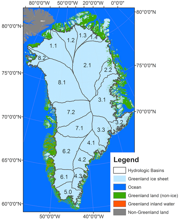
Approximately 80% of Greenland is permanently covered by ice (i.e. the Greenland Ice Sheet), leaving only ~20% of the perimeter inhabitable by humans, animals and vegetation (Fig. 1). Our study area included both the land and ice-covered regions of Greenland with specific focus on the terrestrial land and vegetated areas. Although small, Greenland's vegetated areas are of primary importance to its indigenous population. Subsistence hunting is a significant aspect of both their livelihood strategies and their cultural identity (Andersen and Poppel, Reference Andersen and Poppel2002). It is well documented that the ice-covered regions of Greenland have experienced major changes in the past two decades including more than quadrupling its mass loss (e.g. −142 ± 49 gigatonnes per year from 1992 to 2011; Shepherd and others, Reference Shepherd2012) and increasing surface melt and subsequent runoff (e.g. Enderlin and others, Reference Enderlin2014).

Fig. 1. This study focuses on terrestrial Greenland (green) and associated ice sheet hydrological basins (Zwally and others, Reference Zwally, Giovinetto, Beckley and Saba2012) that deliver meltwater to this area. Together the sub-basins make up the larger basins that are referred to in the text (e.g. sub-basins 6.1 and 6.2 make up basin 6.0; 8.1 and 8.2 comprise 8.0, etc.).
DATA AND METHODS
Remote-sensing data
For this analysis, three different Level 3 MODIS products were employed. These included the 250 m MODIS 16 d composite Vegetation Product (MOD13Q1 – Huete and others, Reference Huete2002), the daily 500 m Snow Cover Product (MOD10A1 – Hall and others, Reference Hall, Riggs, Salomonson, DiGirolamo and Bayr2002) and the daily 1 km LST/emissivity product (MOD11A1 – Wan, Reference Wan2008). All data were from Collection 5, and all tiles comprising the land surface of Greenland were used when available (h15v02–03; h16v00–02; h17v00–03). For each collection, all available tiles from 2000 to 2014 from Julian days 087–305 were used. These data were freely available and were obtained from NASA's Earthdata website.
Vegetation data
The 250 m NDVI subset of MOD13Q1 was used to estimate the productivity of Greenlandic vegetation (Solano and others, Reference Solano, Didan, Jacobson and Huete2010). NDVI is a normalized, band ratio algorithm (Tucker, Reference Tucker1979) and was calculated as:
 $${\rm NDVI} = \displaystyle{{\rho _{{\rm b}2} - \rho _{{\rm b}1}} \over {\rho _{{\rm b}2} + \rho _{{\rm b}1}}},$$
where ρ b1 was MODIS band 1 (0.620–0.670 µm) and ρ b2 was MODIS band 2 (0.841–0.876 µm) on the MODIS Terra instrument. This product is a 16 d composite corresponding with the maximum NDVI value with the smallest sensor view angle obtained during the 16 d observation period. Sellers (Reference Sellers1985) demonstrated that NDVI is a near linear indicator of photosynthetic capacity in vegetation. This fact, in combination with the high temporal sampling frequency of sensors like the Advanced Very High Resolution Radiometer (AVHRR), and the relatively long time series (for satellite data) has meant that NDVI has most widely used vegetation index for remote-sensing phenological studies, particularly in the Arctic (e.g. Jia and others, Reference Jia, Epstein and Walker2009; Bhatt and others, Reference Bhatt2010).
Snow data
The 500 m Fractional Snow Cover (FSC) data from the MOD10A Daily Snow Product (Riggs and others, Reference Riggs, Hall and Salomonson2006) was used to estimate the length of the SFP for terrestrial Greenland. This product uses the Normalized Difference Snow Index (NDSI; Dozier, Reference Dozier1989) and an empirical regression equation (Salomonson and Appel, Reference Salomonson and Appel2004) to estimate the fraction of snow covering (FSC) individual pixels in the scene. The NDSI and the FSC were calculated as:
 $$NDSI = \displaystyle{{\rho _{b6} - \rho _{b4}} \over {\rho _{b6} + \rho _{b4}}}$$
 $$FSC = 0.06 + 1.21 \times NDSI$$
where ρ b4 was band 4 (0.545–0.565 µm) and ρ b6 was band 6 (1.628–1.652 µm) from MODIS Terra.
Temperature data
The 1 km daily, daytime LST data from MOD11A1 were also used in this analysis (Wan, Reference Wan2007). These data estimate LSTs using MODIS infrared bands and a generalized split window algorithm (Wan and Dozier, Reference Wan and Dozier1996). The accuracy of these data have been assessed, with Wan (Reference Wan2008) reporting that the remotely sensed LST data were within 1°C of actual temperatures in most cases when compared against in situ data. These data have been used to estimate LSTs for agriculture (Coll and others, Reference Coll2005), lakes (Wan and others, Reference Wan, Zhang, Zhang and Li2002), and ice sheets (Hall and others, Reference Hall2013). They have also been employed to estimate evapotranspiration in agricultural systems (McCabe and Wolock, Reference McCabe and Wolock2010).
Spatial data and masks
Several other ancillary remotely sensed datasets were also used in this analysis. These included: the 250 m MODIS and SRTM derived land water mask (MOD44W - Carroll and others, Reference Carroll, Townshend, DiMiceli, Noojipady and Sohlberg2009); the mosaic of Greenland (MOG - Haran and others, Reference Haran, Bohlander, Scambos, Painter and Fahnestock2013); elevation data from the Greenland Ice Mapping Project (GIMP - Howat and others, Reference Howat, Negrete and Smith2014); and the Greenland Ice Sheet drainage basin data (Zwally and others, Reference Zwally, Giovinetto, Beckley and Saba2012). These data were used to separate land from ice and water and they were also used to subset Greenland into regions of interest for the study.
Land surface descriptors
Deriving snow seasonality descriptors
Snow seasonality descriptors were derived using the FSC subset of the MOD10A1 data (Salomonson and Appel, Reference Salomonson and Appel2004; Riggs and others, Reference Riggs, Hall and Salomonson2006). Descriptors for the SFP were derived using the snow cover melt date (SCMD) in the spring and the onset of snow cover (SCOD) in the fall (Fig. 2). The duration of the SFP was calculated directly from SCMD and SCOD as:
 $${\rm SFP} = {\rm SCMD} - {\rm SCOD}{\rm.} $$
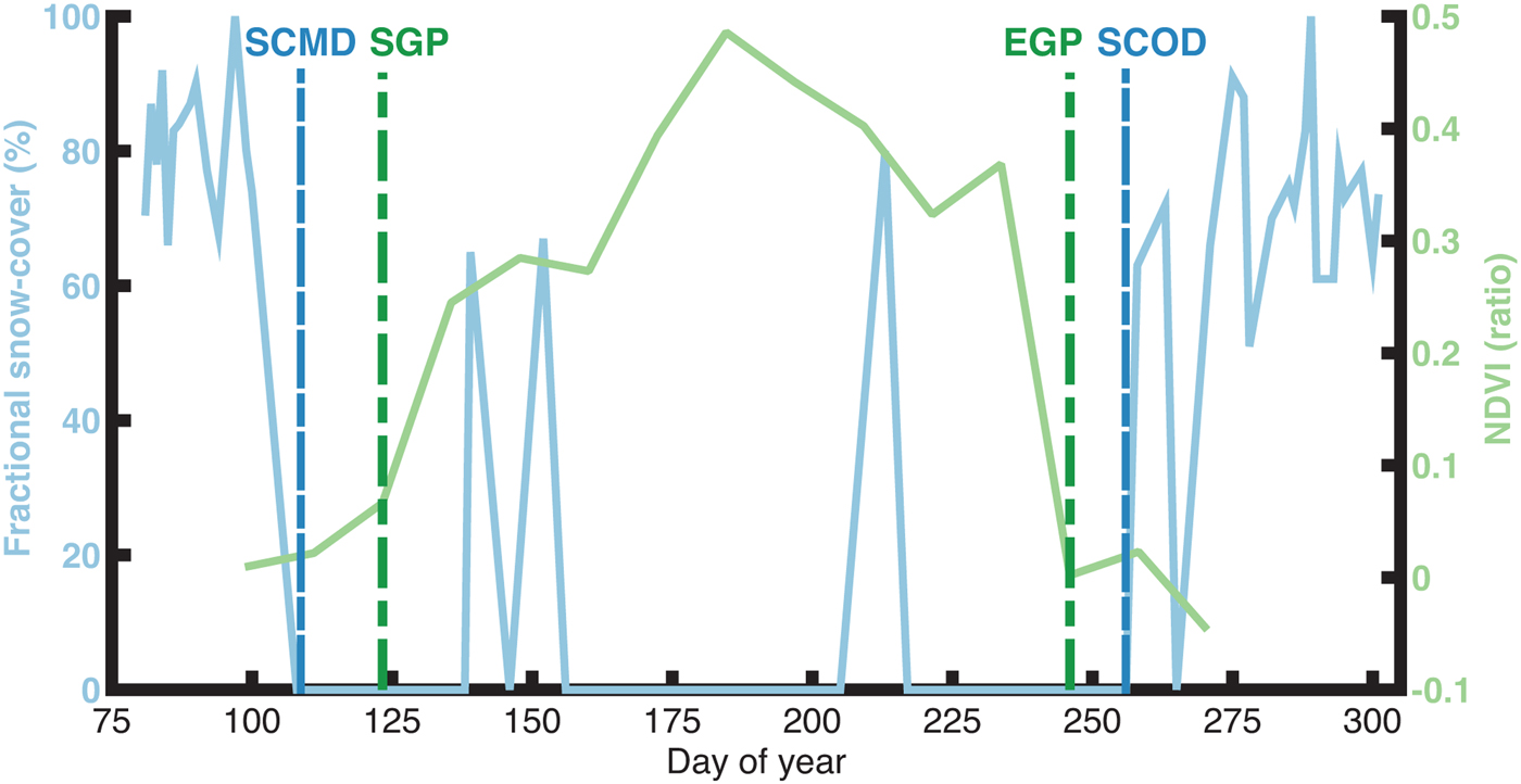
Fig. 2. Schematic representation illustrating the relationship between the snow cover descriptors (vertical blue lines; Snow Cover Melt/Onset Date) estimated using the Fractional Snow Cover data (blue line) and the vegetation phenology descriptors (vertical green lines; Start/End of Growing Period) estimated using the Normalized Difference Vegetation Index data (green line).
Here the snow seasonality descriptors were defined on a per pixel basis. The descriptor corresponding with seasonal SCMD was identified as the first day that the MOD10A1 FSC product reported snow cover as having disappeared (FSC = 0%). Similarly, the descriptor date corresponding with SCOD was the last date in the year that a pixel was observed to be snow-free (FSC = 0%).
Deriving vegetation phenology and productivity descriptors
Vegetation phenology and productivity descriptors were derived from the MOD13q1 NDVI data. Descriptors corresponding with the start of the growing period (SGP), end of the growing period (EGP), duration of the growing period (DGP) and vegetation productivity were also estimated on a per pixel basis. SGP and EGP were estimated using thresholds derived from an averaged NDVI time series of vegetated areas around Greenland. The derivation of the threshold and the averaged time series are described in the Supplementary Materials (Fig. S3). The threshold applied to each was calculated as:
 $${\rm Theshol}{\rm d}_{{\rm NDVI}} = {\rm Rang}{\rm e}_{{\rm NDVI}} \times {\rm \;} 0.30 + {\rm Minimum}_{{\rm NDVI}},$$
where the RangeNDVI was the average range of the average NDVI time series (Fig. S3) and MinimumNDVI was the average minimum from this time series. These averages were estimated directly from Fig. S3, and the threshold used here was 0.06. This was ~10% of the average maximum NDVI values from the vegetated ROI pixels in Figure 1.
It is well known that the presence of on ground snow cover artificially depresses the NDVI signal (Huete and others, Reference Huete2002), thereby influencing the determination of phenological descriptor dates from remotely sensed imagery (Justice and others, Reference Justice, Holben and Gwynne1986; Myneni and others, Reference Myneni, Keeling, Tucker, Asrar and Nemani1997). For this reason, additional constraints were used in conjunction with the NDVI threshold to estimate the land surface phenology descriptors. The snow seasonality descriptors were also used to determine when a given pixel was within the SFP. The SGP date was defined as the first date in the SFP that the NDVI value was ≥0.06 and the EGP date was defined as the last date in the SFP that the NDVI value was ≥0.06. Land surface phenology descriptors were only derived for vegetated pixels, as described in the Supplementary Materials.
In addition to the descriptors corresponding with the start and end of the growing period, the productivity of the vegetation was also estimated. Productivity was approximated using the area under the seasonal NDVI curve (time-integrated NDVI; TI-NDVI). The TI-NDVI provided an assessment of a pixel's gross primary productivity, and is an important phenological descriptor of vegetation dynamics (Reed and others, Reference Reed1994). Yearly comparisons of TI-NDVI values provide an estimate of inter-annual differences in vegetative productivity from year to year. Bhatt and others (Reference Bhatt2013) used several years of TI-NDVI data from an AVHRR image time series to characterize climate relative changes in vegetation productivity across the pan-Arctic region. Whereas the AVHRR data employed by Bhatt and others (Reference Bhatt2013) have a relatively coarse spatial resolution (~5 × 5 km), the MOD13q1 data used here have comparatively finer spatial resolution (250 × 250 m).
Estimating accumulated growing degree-days
The numbers of accumulated growing degree-days (AGDD) were estimated for each vegetated pixels using MOD11A1 data. Photosynthesis is a temperature-sensitive biological process (Nobel, Reference Nobel2009) and temperatures <0°C generally suppressed plant growth. Below this temperature, plants have a limited ability to produce catalytic enzymes required for photosynthetic processes (Kirschbaum and Farquhar, Reference Kirschbaum and Farquhar1984), which suppresses tissue formation (Körner, Reference Körner1998). Here, AGDD were defined as the number of days during the SFP when the LST > 0°C were recorded. This descriptor was also defined on a per pixel basis for each year and was derived from the daytime LST observations.
Sensitivity analysis
There were two major sources of uncertainty associated with the derived remotely sensed snow seasonality and vegetation phenology descriptors described above. Firstly, melting snow cover influences NDVI time series. In particular, it influences the derivation of both the SGP and EGP descriptors (Reed and others, Reference Reed, White and Brown2003, Reference Reed, Budde, Spencer and Miller2009; White and others, Reference White2009). A sensitivity analysis was performed to determine what effect the selection of different FSC thresholds had on the derivation of phenological descriptor dates. The details of this analysis are in the Supplementary Materials.
In addition, changes in cloud climatology can confound the results of remote-sensing studies. Snow/cloud misclassification remains a perennial challenge in optical remote sensing (e.g. Hall and Riggs, Reference Hall and Riggs2007). Because optical sensors cannot penetrate cloud cover in areas with increasing cloud cover, there is uncertainty regarding the status of the land surface. Here, trends in the number of cloudy days were also assessed (Supplementary Materials). These results were used to inform subsequent investigations, specifically the joint descriptor analysis for individual drainage basins (section ‘Basin-wide trend analysis’).
Analytical methods
Greenland-wide trend analysis
To understand how increased energy inputs associated with Arctic amplification were impacting vegetation, we calculated long-term averages for each of the three individual descriptors (SFP, TI-NDVI and AGDD) using the time series of all vegetated pixels. For each year, we counted both the number of pixels that exceeded (≥) or fell below (<) the long-term average of each descriptor. The yearly counts were then analyzed to determine whether or not the proportion of pixels in each category remained stable across the study period. The temporal trends in those counts were assessed using generalized linear models from the Statistics Toolbox of MATLAB (MathWorks, 2016).
In addition to the analysis of the individual snow seasonality and vegetation phenology descriptors, we also undertook a similar analysis of joint descriptors. For this, we examined pair-wise combinations of the descriptors (e.g. TI-NDVI and AGDD; AGDD and SFP; SFP and TI-NDVI). For each year, we counted the number of pixels above (≥) and below (<) the long-term averages of both descriptors. Temporal trends related to the fraction of pixels in each joint class were also assessed using generalized linear models from the Statistics Toolbox of MATLAB (MathWorks, 2016).
Basin-wide trend analysis
In addition to the analysis of vegetated areas around Greenland, a similar analysis was performed for individual drainage basins in Western Greenland (Fig. 1). Basins in Eastern Greenland were not included in this analysis, as the analysis of cloud cover (Supplementary Materials) revealed there was a substantial increase in the number of cloudy days that occurred during the study. As with the Greenland-wide analysis, the long-term basin averages for each descriptor were used to assess the yearly fraction of pixels in the basin that exceed (≥) and fell below (<) the long-term average. Trends in the descriptors were assessed for the individual basins using generalized linear models from the Statistics Toolbox of MATLAB (MathWorks, 2016).
Mapped results
Spatial patterns in the yearly joint comparisons (section ‘Deriving vegetation phenology and productivity descriptors’) were also analyzed by mapping the results of the joint analysis (section ‘Greenland-wide trend analysis’). Results from Hall and others (Reference Hall2013) were used to identify years where temperatures across the Greenland Ice Sheet were: cooler (2000), average (2004) and warmer than usual (2010). Although Hall and others (Reference Hall2013) only examined ice surface temperatures in their study, it was thought the atmospheric conditions influencing ice surface temperatures in those years would likely have also affected LSTs off the ice in a similar manner.
RESULTS
Greenland-wide trends in snow seasonality, growing degree-days and vegetation descriptors
The results indicated that most vegetated surfaces experienced an increase in AGDD throughout the study period (Fig 3b). For the joint descriptors, the results indicated an increase in the proportions of pixels that experienced both longer SFPs and more cumulative growing degree-days (Fig. 4b). The pattern for AGDD and vegetation productivity was similar (Fig. 4c), and neither result was statistically significant as there was considerable inter-annual variability evident (Figs 4b and c). There was a statistically significant increase in the number of pixels that experienced both an increase in AGDD and reduced vegetation productivity (Fig. 4f).

Fig. 3. (a) Changes in the percentage of vegetated pixels in Greenland that experienced longer than average duration of the snow-free period (SFP) from 2000 to 2014; (b) changes in the percentage of vegetated pixels that experienced more accumulated growing degree-days (AGDD) from 2000 to 2014; (c) changes in the percentage of vegetated pixels that exhibited above-average time-integrated NDVI (TI-NDVI) from 2000 to 2014. Solid lines represent the linear trends in the data; dashed lines represent the uncertainty (95% confidence level) associated with the trends. Significance code: *p ≤ 0.05.

Fig. 4. (a) Changes in the percentage of vegetated pixels in Greenland that experienced both longer than average snow-free periods (SFP) and exhibited increased vegetation productivity (TI-NDVI); (b) changes in the percentage of pixels that experienced both above average SFP and increased numbers of accumulated growing degree-days (AGDD); (c) changes in the percentage of pixels that experienced both increased numbers of AGDD and exhibited increased TI-NDVI; (d) percentage of vegetation pixels that experienced above average duration of the SFP and also exhibited decreased TI-NDVI; (e) percentage of vegetation pixels experiencing both above average SFP and reduced numbers of AGDD; (f) percentage of vegetation pixels that experienced increased AGDD and exhibited reduced TI-NDVI. Solid lines represent the linear trends in the data; dashed lines represent the uncertainty (95% confidence level) associated with the trends. Significance codes: **p ≤ 0.01; *p ≤ 0.05.
Basin-wide trends in snow seasonality, growing degree-days, and vegetation descriptors
The full results for the basin-wide analysis are presented in the Supplementary Materials (Figs S5–S7), and only the joint descriptor results for basins 5 and 6 are presented in Figure 5. These were the only basins where statistically significant results were observed. Both basins experienced a reduction in the number of pixels that experienced longer than average SFPs and fewer numbers of growing degree-days (Figs 5b and c). Both basins had an increase in pixels with longer SFPs and reduced vegetation productivity during the study period (Figs 5e and f).
Fig. 5. (a) Changes in the percentage of vegetated pixels in basins 5.0 and 6.0 with longer than average SFP that also exhibited reduced TI-NDVI; (b) changes in the percentage of pixels that experienced both longer than average SFP and reduced numbers of AGDD; and (c) changes in the percentage of pixels that experienced increased numbers of AGDD and exhibited reduced TI-NDVI. Solid lines represent the linear trends in the data; dashed lines represent the uncertainty (95% confidence level) associated with the trends. Significance codes: **p ≤ 0.01; *p ≤ 0.05.
Maps results for the joint snow seasonality, growing degree-days, and vegetation descriptors
Mapped results of the joint descriptor analysis for a cool (2000), average (2004) and a warm year (2010) are presented in Figure 6. In the cool and warm years, most of the pixels in Western Greenland had descriptor values that were lower than average (cool; 2000) or higher than average (warm; 2010). In 2000, purple pixels featured prominently in all three maps in the cool year (2000) indicating ubiquitously low values for all of the descriptors. In contrast, in 2010, orange pixels dominated the map, which indicated a ubiquity of higher than average descriptor values. In 2010, the areas where the longer SFPs resulted in more growing degree-days and lower productivity (black areas for 2010, right most map Fig. 6) were also readily observed, particularly in Western Greenland.
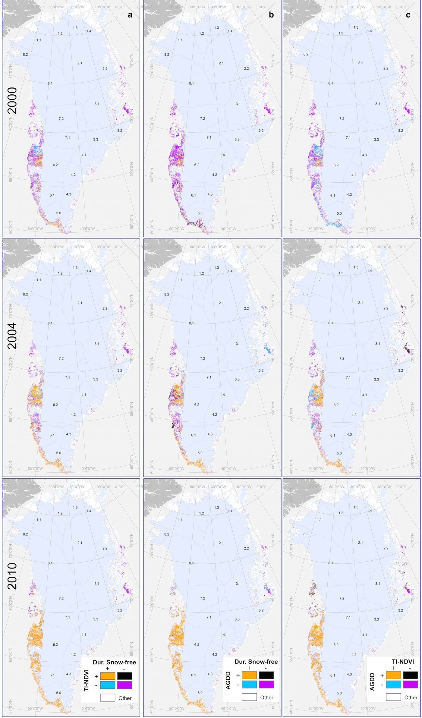
Fig. 6. Mapped results for the joint descriptor analysis representing combinations of higher (+)/lower (−) than average: (a) time-integrated NDVI (TI-NDVI) and duration of the snow-free period (SFP); (b) accumulated growing degree-days (AGDD) and duration of the snow-free period (SFP); and (c) accumulated growing degree-days (AGDD) and time-integrated NDVI (TI-NDVI). Patterns were representative of a cool (2000), an average (2004) and a warm year (2010) within the time series. A larger version of this map is included in the Supplementary Materials.
DISCUSSION
This study had two major aims. Firstly, we wanted to determine whether or not longer SFPs were causing terrestrial Greenlandic vegetation to dry out. If there was evidence for the drying hypothesis, a subsequent aim of the study was to determine how extensive the drying phenomenon was. The results for the whole of Greenland indicated that ~45% of the vegetated areas experienced increased SFPs that also coincided with an increase in AGDD (Fig. 4b). For many areas, this increase in growing degree-days also resulted in higher vegetation productivity (Fig. 4c). In others areas, more AGDD resulted in decreased productivity across the study period (Fig. 4f). This later result was statistically significant, and was consistent with the drying hypothesis.
Overall, ~25% of the vegetated areas across Greenland experienced lower than average productivity. Although this phenomenon was not pervasive across the study period (as much as 60% of vegetated pixels experienced higher than average productivity in 2010; Fig. 4c), this result is important. In the southernmost basins (5–6), a statistically significant change in vegetation productivity was observed (Fig. 5c). In basins 5 and 6, average productivity declined across the study period, even though they also experienced more growing degree-days than average. This phenomenon is consistent with the drying hypothesis.
The results presented here suggested that changes associated with increased energy inputs are potentially more complex than originally predicted by the Budyko (Reference Budyko1974) framework. The combination of longer SFPs and more AGDD should have resulted in higher vegetation productivity, according to the framework. The framework does not account for the fact that some pixel's productivity decreased when they were exposed to increased energy inputs and experienced similar climatic conditions as the pixels where productivity increased. Local hydrologic changes represent one possible explanation, as vegetation still requires access to water in order to maintain or increase productivity. Our results suggest that water stress may play an increasingly important role in maintaining vegetation productivity in some areas of Greenland (e.g. basins 5–6; Fig. 5c). For these areas, micro-meteorological and local environmental conditions are likely more influential drivers of vegetation phenology than mesoscale and synoptic scale warming associated with Arctic amplification.
What remains unclear is what ultimately contributed to the reduction in vegetation productivity that was observed in these basins. Interestingly, in basins 5 and 6, many areas where decreased productivity was observed were situated closer to the edge of the ice sheet (Fig. 6c). Whether or not this corresponded with changes in precipitation during study period is unclear; exploratory modeling of the data (not presented) did not yield any conclusive results in this regard. It is possible that the reductions in vegetation productivity were associated with localized phenomena. Foehn (or, adiabatically warmed katabatic) winds are one possible explanation. In Greenland, it has long been observed that localized warming associated with foehn winds can dramatically reduce snow cover over relative short periods (Thing, Reference Thing1984). When precipitation falls, the temperature of air parcels that previously contained moisture increases. As these parcels subsequently descend to lower elevations, they add additional heat to the land surface. This can melt snow cover (Thing, Reference Thing1984), which is an important driver of vegetation phenology in the Arctic. Foehn winds could account for the localized reductions in vegetation productivity that we observed in this study, particularly in areas close to the ice sheet. Investigating this possibility represents a possible avenue for further research.
While our results appeared to support the drying hypothesis, there were some limitations with this study. One limitation related to the use of the fractional snow cover data. The MOD10A1 FSC product tends to underestimate the amount of snow cover within a pixel, particularly in the transitions into and out of the snow-covered period (Rittger and others, Reference Rittger, Painter and Dozier2013). This could have biased our estimates for the duration of the SFP. However, the sensitivity analysis (Supplementary Results) indicated that using different snow cover thresholds did not substantially affect the snow seasonality descriptor dates. As a result, it is unlikely that potential bias in MOD10A1 FSC data would significantly impact the results presented here.
The use of NDVI time series to assess vegetation phenology represents another potential limitation associated with this study. When present, NDVI signals are attenuated by both snow cover and water. As previously noted, our algorithm tried to minimize these effects but it is possible that some sub-pixel snow cover or water was present within some vegetated pixels during the study period. Medium- to long-term changes in small persistent water bodies would be particularly problematic for this analysis. They would depress the NDVI signal through time, thereby reducing the yearly TI-NDVI signal. It would be difficult to differentiate the effects of sub-pixel water accumulation from that of drying vegetation using NDVI. This represented another limitation of our study.
We do not think sub-pixel water accumulation significantly impacted our results. The spatial patterns we observed in our results were similar to those presented by Watts and others (Reference Watts, Kimball, Bartsch and McDonald2014) in their study of open water in the Arctic. A visual inspection of our results with the trend analysis presented by Watts and others (Reference Watts, Kimball, Bartsch and McDonald2014) revealed that the areas where we observed decreasing productivity were similar to the areas where those authors reported that the fraction of open water decreased throughout their study. Differences in spatial resolutions and study periods precluded direct quantitative comparisons of the results presented here and those reported by Watts and others (Reference Watts, Kimball, Bartsch and McDonald2014). However, the visual similarities in both results suggest that water accumulation did not unduly influence our analysis, though it does warrant further investigation. A quantitative comparison could serve as an independent validation of our findings and this represents another potential avenue for future research.
CONCLUSION
This study used three image time series obtained by MODIS to determine whether or not longer SFPs might be causing terrestrial vegetation to dry out in Greenland. In some vegetated areas, the remotely sensed observations were consistent with the drying hypothesis. Drying affected ~25% of Greenland's vegetated pixels, and was more pronounced in basins located in Southwestern Greenland. Our results also suggest that the localized impacts associated with drying were more nuanced than could be predicted by the Budyko (Reference Budyko1974) eco-hydrological framework.
SUPPLEMENTARY MATERIAL
The supplementary material for this article can be found at https://doi.org/10.1017/aog.2018.24
ACKNOWLEDGEMENTS
J.A.T. was supported by the Postdoctoral Visiting Fellowship Program at the Cooperative Institute for Research in Environmental Sciences at the University of Colorado. J.A.T. wishes to thank Mahsa Mousavi and Alan Pope for discussions and helpful comments, and Karl Rittger for helpful MATLAB suggestions throughout the project. We thank the reviewers for their thoughtful and insightful comments, which greatly helped improve the manuscript. We are not aware of any conflicts of interest regarding this work. Publication of this article was funded by the University of Colorado Boulder Libraries Open Access Fund.


 Open access