


Introduction
The Antarctic Peninsula (AP) is one of the fastest-warming locations in the world and is experiencing rapid environmental changes (Vaughan et al. Reference Vaughan, Marshall, Connolley, Parkinson, Mulvaney and Hodgson2003, Ruiz-Fernandez et al. Reference Ruiz-Fernandez, Oliva, Nyvlt, Cannone, Garcia-Hernandez and Guglielmin2019, Turner et al. Reference Turner, Holmes, Harrison, Phillips, Jena and Reeves-Francois2022, Siegert et al. Reference Siegert, Bentley, Atkinson, Bracegirdle, Convey and Davies2023). Late Holocene palaeoenvironmental data are crucial for placing these observations of modern changes into context. Holocene climate events across the AP are recorded in high-resolution marine, lacustrine and ice-core records (Michalchuk et al. Reference Michalchuk, Anderson, Wellner, Manley, Majewski and Bohaty2009, Mulvaney et al. Reference Mulvaney, Abram, Hindmarsh, Arrowsmith, Fleet and Triest2012, Sterken et al. Reference Sterken, Roberts, Hodgson, Vyverman, Balbo and Sabbe2012, Totten et al. Reference Totten, Anderson, Fernandez and Wellner2015, Cejka et al. Reference Cejka, Nyvlt, Kopalova, Bulinova, Kavan and Lirio2020, Groff et al. Reference Groff, Beilman, Yu, Ford and Xia2023). Proxy data from these cores record past periods of warming and cooling driven by wind shifts, ocean circulation changes and El Niño-Southern Oscillation (ENSO) variability (Domack et al. Reference Domack, Leventer, Dunbar, Taylor, Brachfeld and Sjunneskog2001, Shevenell et al. Reference Shevenell, Ingalls, Domack and Kelly2011, Barbara et al. Reference Barbara, Crosta, Leventer, Schmidt, Etourneau, Domack and Massé2016, Nie et al. Reference Nie, Xiao and Wang2022). However, these proxy reconstructions only indirectly record environmental changes occurring within the coastal zone. One underutilized palaeoenvironmental proxy is the sedimentary characteristics of beach deposits (Scheffers et al. Reference Scheffers, Engel, Scheffers, Squire and Kelletat2012, Lindhorst & Schutter Reference Lindhorst and Schutter2014, Simkins et al. Reference Simkins, Simms and DeWitt2015), which along most Antarctic coastlines have been uplifted and thus preserved due to post-glacial rebound. Because these beach deposits reflect coastal environmental characteristics such as wave climate, sea-ice cover and iceberg density (Hall & Perry Reference Hall and Perry2004, Simkins et al. Reference Simkins, Simms and DeWitt2015), changes in their characteristics may reflect environmental changes occurring within the coastal zone through the Holocene.
The purpose of this study is to characterize trends in ground-penetrating radar (GPR) profiles, gross morphology, grain size, clast roundness and ice-rafted debris (IRD) on raised beach deposits through the late Holocene on Joinville Island along the Eastern Antarctic Peninsula (EAP; Fig. 1). Changes in these proxies through time are hypothesized to reflect changes in the processes operating on beaches through the late Holocene and thus to reflect the environmental changes impacting the area. This archive also augments studies of palaeo-sea levels (e.g. Zurbuchen & Simms Reference Zurbuchen and Simms2019) derived from the same raised beaches by providing ages for the older beach ridges and a background as to what other changes may be responsible for beach-ridge elevation changes.
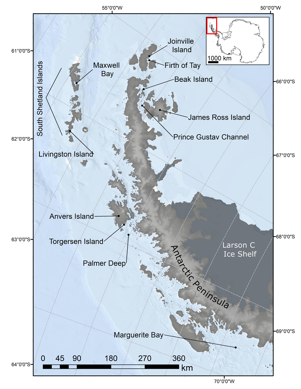
Fig. 1. Map showing the location of the field site and other places mentioned in the text.
Background
Beaches as potential archives of past environmental conditions
Wave climate provides a first-order control on beach deposit characteristics (Butler Reference Butler1999). Thus, the granulometry of beach deposits may provide a proxy archive of environmental conditions impacting wave climate through time (Bentley et al. Reference Bentley, Hodgson, Smith and Cox2005, Simkins et al. Reference Simkins, Simms and DeWitt2015). The presence of sea ice restricts wave exposure and sediment supply to the beach (Nichols Reference Nichols1961, Butler Reference Butler1999) by limiting fetch, thus decreasing wave energy. Therefore, in the absence of significant fluvial sources in the area, cooler conditions associated with sea ice and the less frequent reworking of beach cobbles are thought to be characteristic of beach deposits with more poorly rounded clasts (Nichols Reference Nichols1961, Butler Reference Butler1999, Simkins et al. Reference Simkins, Simms and DeWitt2015). Warmer conditions associated with no sea ice and higher wave energy are thought to be characteristic of beach deposits consisting of more rounded clasts (Nichols Reference Nichols1961).
IRD prevalence is another aspect of beach deposits that provides an archive of past environmental conditions. Hall & Perry (Reference Hall and Perry2004) used IRD on Byers Peninsula of Livingston Island in the South Shetland Islands to create a climate proxy for the northern AP during the Holocene. The proxy is based on IRD densities from boulder counts along beach ridges. Higher IRD counts were interpreted to represent cooler climate conditions marked by glacial advances (Hall & Perry Reference Hall and Perry2004), whereas lower IRD counts were interpreted to represent warmer conditions and glacial retreat (Kanfoush et al. Reference Kanfoush, Hodell, Charles, Janecek and Rack2002).
Modern climate and oceanographic setting
The EAP is subjected to cold, saline Weddell Sea Transitional Waters from the Weddell Gyre (García et al. Reference García, Castro, Rıos, Doval, Rosón, Gomis and López2002) and is associated with cold continental air masses (Reynolds Reference Reynolds1981) and extensive sea ice (Stammerjohn & Smith Reference Stammerjohn and Smith1996, Domack et al. Reference Domack, Leventer, Root, Ring, Williams and Carlson2003, Ingólfsson et al. Reference Ingólfsson, Hjort and Humlum2003, Michalchuk et al. Reference Michalchuk, Anderson, Wellner, Manley, Majewski and Bohaty2009). Clockwise circulation of the Weddell Gyre brings warm Circumpolar Deep Water into the EAP (Orsi et al. Reference Orsi, Nowlin and Whitworth III1993), turning the Circumpolar Deep Water into Weddell Sea Transitional Water (Barbara et al. Reference Barbara, Crosta, Leventer, Schmidt, Etourneau, Domack and Massé2016, Vernet et al. Reference Vernet, Geibert, Hoppema, Brown, Haas and Hellmer2019). The Antarctic Sound to the west of Joinville Island is a zone of mixing between Weddell Sea waters and those from the Bransfield Basin, with waters from the Bransfield Basin being more dominant during the summer months (Krek et al. Reference Krek, Krek, Krechik, Morozov, Flint and Spiridonov2021).
Due to its extensive sea ice, the influence of southern barrier winds and fewer oceanic connections with the Pacific Ocean, the Weddell Sea sector of the AP is much cooler than other parts of the AP (Ambrozova et al. Reference Ambrozova, Laska and Kavan2020). The coldest temperatures are recorded when winds are out of the south, whereas they are warmer when the winds blow from the north (Ambrozova et al. Reference Ambrozova, Laska, Hrbacek, Kavan and Ondruch2019). These southerly winds are sometimes referred to as ‘barrier winds’ and are sourced from the interior of the continent to the south of the Weddell Sea and kept on the EAP due to the presence of the mountains of the AP (Schwerdtfeger Reference Schwerdtfeger1975). The EAP is less influenced by westerly winds, which are a key climate driver across West Antarctica (Marshall et al. Reference Marshall, Orr, van Lipzig and King2006), than the western AP because the mountains located along the AP act as a barrier to winds and ocean currents (Bentley et al. Reference Bentley, Hodgson, Smith, Cofaigh, Domack and Larter2009, Dickens et al. Reference Dickens, Kuhn, Leng, Graham, Dowdeswell and Meredith2019). However, landmasses and surrounding bodies of water located at the northeastern tip of the AP might not be completely shielded or isolated from western influences due to low relief of the islands and oceanographic connections (Michalchuk et al. Reference Michalchuk, Anderson, Wellner, Manley, Majewski and Bohaty2009, Krek et al. Reference Krek, Krek, Krechik, Morozov, Flint and Spiridonov2021).
The Weddell Sea contains the largest accumulation of multiyear sea ice in the Southern Ocean, accounting for over a third of the total sea ice in the Southern Ocean (Parkinson & Cavelleri Reference Parkinson and Cavalleri2012). After a steady increase in sea-ice extent through the latter half of the twentieth century, sea ice started to experience an abrupt decrease in extent after 2015, with several record low extents being noted since that time (Kumar et al. Reference Kumar, Yadav and Mohan2021, Parkinson & DiGirolamo Reference Parkinson and DiGirolamo2021, Jena et al. Reference Jena, Bajish, Turner, Ravichandran, Anilkumar and Kshitija2022). Those trends vary according to season, with a general increase occurring during summer months and a decrease occurring during winter months (Kumar et al. Reference Kumar, Yadav and Mohan2021). Some of these recent minimum sea-ice extents have been linked to intense storms (Jena et al. Reference Jena, Bajish, Turner, Ravichandran, Anilkumar and Kshitija2022).
Ongoing and past climate changes
Climate in the AP region behaves differently than in the continental interior of Antarctica. Although shifts in westerly winds and the Antarctic Circumpolar Current caused rapid sea-ice retreat in the western AP during the Holocene (Shevenell et al. Reference Shevenell, Ingalls, Domack and Kelly2011, Mulvaney et al. Reference Mulvaney, Abram, Hindmarsh, Arrowsmith, Fleet and Triest2012, Barbara et al. Reference Barbara, Crosta, Leventer, Schmidt, Etourneau, Domack and Massé2016), Barbara et al. (Reference Barbara, Crosta, Leventer, Schmidt, Etourneau, Domack and Massé2016) suggest that the EAP responded differently than the western AP because of the presence of the Weddell Gyre. Instead, the circulation of the gyre transported more fresh, cold surface waters and sea ice northwards, which slowed ice-shelf retreat on the EAP and delayed seasonal open water conditions. However, warming and sea-ice demise have since continued on both sides of the AP over the last 5 years (e.g. Kumar et al. Reference Kumar, Yadav and Mohan2021).
Over the Holocene, forcing mechanisms produced shifts in climatic conditions, including the Early Holocene Climate Optimum, the Mid-Holocene Warm Period, the Neoglacial interval, the Mediaeval Warm Period, the Little Ice Age (LIA) and the recent rapid regional warming period (Bentley et al. Reference Bentley, Hodgson, Smith, Cofaigh, Domack and Larter2009). However, the various proxy records do not all record each of these climate periods. The absence of climatic events might be caused by the analysis of different proxy records. For example, a marine core taken from the Palmer Deep, Site IODP 1098, records the LIA at ~0.70–0.15 ka (Domack et al. Reference Domack, Leventer, Dunbar, Taylor, Brachfeld and Sjunneskog2001, Domack et al. Reference Domack, Leventer, Root, Ring, Williams and Carlson2003), whereas marine cores taken from the Firth of Tay and Maxwell Bay have no pronounced records of the LIA (Michalchuk et al. Reference Michalchuk, Anderson, Wellner, Manley, Majewski and Bohaty2009, Milliken et al. Reference Milliken, Anderson, Wellner, Bohaty and Manley2009), even though terrestrial records nearby show clear evidence for a LIA (Kaplan et al. Reference Kaplan, Strelin, Schaefer, Peltier, Martini and Flores2020, Simms et al. Reference Simms, Bentley, Simkins, Zurbuchen, Reynolds, DeWitt and Thomas2021).
Bentley et al. (Reference Bentley, Hodgson, Smith, Cofaigh, Domack and Larter2009) described each of the Holocene climate periods. The Early Holocene Climate Optimum lasted from 11.0 to 9.5 ka (Johnson et al. Reference Johnson, Bentley, Roberts, Binnie and Freeman2011). This period is characterized by significant widespread warming (Masson-Delmotte et al. Reference Masson-Delmotte, Stenni and Jouzel2004) and ice retreat across Antarctica during the early Holocene (Pudsey et al. Reference Pudsey, Barker and Larter1994, Domack et al. Reference Domack, Leventer, Dunbar, Taylor, Brachfeld and Sjunneskog2001, Domack Reference Domack2002, Evans et al. Reference Evans, Pudsey, ÓCofaigh, Morris and Domack2005, Bentley et al. Reference Bentley, Hodgson, Smith, Cofaigh, Domack and Larter2009, Davies et al. Reference Davies, Golledge, Glasser, Carrivick, Ligtenberg and Barrand2014, Nyvlt et al. Reference Nývlt, Braucher, Engel and Mlčoch2014). Deglaciation continued, most likely at a slower rate, during the period after the optimum from 9.5 to 4.5 ka, reaching a similar glacial configuration as today sometime around 5–6 ka (Johnson et al. Reference Johnson, Bentley, Roberts, Binnie and Freeman2011, Glasser et al. Reference Glasser, Davies, Carrivick, Rodes, Hambrey, Smellie and Domack2014, Smith et al. Reference Smith, Hillenbrand, Subt, Rosenheim, Frederichs and Ehrmann2021), with there being some geographical variability in climatic responses (Bentley et al. Reference Bentley, Hodgson, Smith, Cofaigh, Domack and Larter2009).
The Mid-Holocene Warm Period, also known as the Mid- to Late Holocene Hypsithermal, was the next climate period of significant warming across the AP from 4.5 to 2.8 ka. This period is associated with rapid sedimentation, high organic productivity and increased species diversity in lake sediments (Björck et al. Reference Björck, Olsson, Ellis-Evans, Håkansson, Humlum and de Lirio1996, Hodgson et al. Reference Hodgson, Doran, Roberts, McMinn, Smol, Pienitz and Douglas2004, Hodgson & Convey Reference Hodgson and Convey2005, Sterken et al. Reference Sterken, Roberts, Hodgson, Vyverman, Balbo and Sabbe2012) and reduced sea-ice coverage, greater primary production and increased marine sedimentation rates (Domack et al. Reference Domack, Leventer, Root, Ring, Williams and Carlson2003, Bentley et al. Reference Bentley, Hodgson, Smith, Cofaigh, Domack and Larter2009, Totten et al. Reference Totten, Anderson, Fernandez and Wellner2015). However, unlike the optimum, not all proxy records across the AP indicate a significant warming trend during this period, and the timing of the Mid-Holocene Warm Period varied by hundreds of years depending upon the proxy (Bentley et al. Reference Bentley, Hodgson, Smith, Cofaigh, Domack and Larter2009).
A shift from warmer conditions to colder conditions marks the end of the Mid-to Late Holocene Warm Period and the start of the Neoglacial period. According to Bentley et al. (Reference Bentley, Hodgson, Smith, Cofaigh, Domack and Larter2009), the Neoglacial interval lasted from ~2.5 to 1.2 ka and probably started earlier on the western AP (3.6 ka; Domack Reference Domack2002) than the EAP (2.5 ka; Bentley et al. Reference Bentley, Hodgson, Smith, Cofaigh, Domack and Larter2009). Cejka et al. (Reference Cejka, Nyvlt, Kopalova, Bulinova, Kavan and Lirio2020) provide a well-documented shift to cooler conditions on the EAP from a lake record on Vega Island that suggests a slightly younger age of ~2.1 ka for the onset of the Neoglacial on the EAP. Shevenell & Kennett (Reference Shevenell and Kennett2002) suggest that the earlier onset in the Palmer Deep was caused by an increase in cooler shelf waters and westerly winds. The climate conditions of this period are associated with more intense sea ice, cooler open water conditions, a decline in biological productivity and a glacial advance (Domack & McClennen Reference Domack and McClennen1996, Totten et al. Reference Totten, Anderson, Fernandez and Wellner2015). Recent mapping (Carrivick et al. Reference Carrivick, Davies, Glasser, Nyvlt and Hambrey2012), modelling (Davies et al. Reference Davies, Golledge, Glasser, Carrivick, Ligtenberg and Barrand2014) and cosmogenic dating of terrestrial moraines has constrained glacial advances to this time period as well (Kaplan et al. Reference Kaplan, Strelin, Schaefer, Peltier, Martini and Flores2020, Palacios et al. Reference Palacios, Ruiz-Fernández, Oliva, Andrés, Fernández-Fernández and Schimmelpfennig2020).
The Neoglacial period is in some places interrupted by the Mediaeval Warm Period, which is thought to have lasted from 1200 to 600 ka and is well documented in the Northern Hemisphere. However, evidence for a Mediaeval Warm Period in Antarctica is fragmentary, with only a few records clearly showing it, and those that do are from the western AP. This evidence includes a few marine core records (Bentley et al. Reference Bentley, Hodgson, Smith, Cofaigh, Domack and Larter2009) and a period of more restricted glacial ice around Palmer Station (Hall et al. Reference Hall, Koffman and Denton2010a, Yu et al. Reference Yu, Beilman and Loisel2016, Charman et al. Reference Charman, Amesbury, Roland, Royles, Hodgson, Convey and Griffiths2018). Evidence for a LIA is growing across the AP. Evidence for the LIA includes glacial advances (Hall Reference Hall2007, Guglielmin et al. Reference Guglielmin, Convey, Malfasi and Cannone2016, Kaplan et al. Reference Kaplan, Strelin, Schaefer, Peltier, Martini and Flores2020, Simms et al. Reference Simms, Bentley, Simkins, Zurbuchen, Reynolds, DeWitt and Thomas2021), increased sea-ice conditions and colder sea-surface temperatures (Domack et al. Reference Domack, Ishman, Stein, McClennen and Jull1995, Bentley et al. Reference Bentley, Hodgson, Smith, Cofaigh, Domack and Larter2009, Hall Reference Hall2009, Shevenell & Kennett Reference Shevenell and Kennett2002). Recent work is beginning to suggest that the timing of the glacial advances within the AP are coeval with the LIA in the Northern Hemisphere (Hall Reference Hall2009, Simms et al. Reference Simms, Bentley, Simkins, Zurbuchen, Reynolds, DeWitt and Thomas2021).
The recent rapid regional warming period, following the LIA, is marked by the ongoing pronounced warming trend across Antarctica, most likely due to increased greenhouse gases in the atmosphere (Houghton Reference Houghton2001). The recent rapid regional warming event is associated with increased sediment accumulation rates in a variety of proxy records such as lake and marine cores (Bentley et al. Reference Bentley, Hodgson, Smith, Cofaigh, Domack and Larter2009), ice retreat, paraglacial changes and reduced sea-ice durations and snow cover (Vaughan et al. Reference Vaughan, Marshall, Connolley, Parkinson, Mulvaney and Hodgson2003, Ruiz-Fernandez et al. Reference Ruiz-Fernandez, Oliva, Nyvlt, Cannone, Garcia-Hernandez and Guglielmin2019, Turner et al. Reference Turner, Holmes, Harrison, Phillips, Jena and Reeves-Francois2022, Siegert et al. Reference Siegert, Bentley, Atkinson, Bracegirdle, Convey and Davies2023).
Regional sea-level reconstructions
Compared to other coastlines, relatively few studies of relative sea-level (RSL) changes are available for much of Antarctica due to limited ice-free locations. The few RSL records that do exist across the AP are found within the South Shetland Islands (Bentley et al. Reference Bentley, Hodgson, Smith and Cox2005, Hall Reference Hall2010, Watcham et al. Reference Watcham, Bentley, Hodgson, Roberts, Fretwell and Lloyd2011, Simms et al. Reference Simms, Ivins, DeWitt, Kouremenos and Simkins2012), Marguerite Bay (Simkins et al. Reference Simkins, Simms and DeWitt2013), Torgersen Island (Simms et al. Reference Simms, Whitehouse, Simkins, Nield, DeWitt and Bentley2018), Alexander Island (Roberts et al. Reference Roberts, Hodgson, Bentley, Sanderson, Milne and Smith2009), Beak Island (Roberts et al. Reference Roberts, Hodgson, Sterken, Whitehouse, Verleyen and Vyverman2011), James Ross Island (Hjort et al. Reference Hjort, Ingólfsson, Möller and Lirio1997) and locally on Joinville Island (Fig. 1; Zurbuchen & Simms Reference Zurbuchen and Simms2019). On Joinville Island, Zurbuchen & Simms (Reference Zurbuchen and Simms2019) reconstructed a record of RSL based on the topographically lower 21 of the 36 beaches on the island. Radiocarbon ages from those lower 18 beach ridges reveal that RSL has fallen 4.9 ± 0.58 m since 3.1 ka, with an abrupt, short-lived increase in the rate of RSL fall from 1.5 to 1.3 ka and a potential RSL rise from 0.7 to 0.2 ka (Zurbuchen & Simms Reference Zurbuchen and Simms2019). The beaches continue to an elevation of 12.2 m, which, when corrected for the 1.3 m elevation of the modern beach ridge crest, suggests a marine limit of no less than 10.9 m, which currently remains undated.
Tay Head peninsula
Joinville Island is located at the north-eastern tip of the AP between D'Urville Island and Dundee Island (Figs 1 & 2). These islands are a geological continuation of the Trinity Peninsula (Elliot Reference Elliot1967). However, due to a combination of snow cover and sparse outcrops, little detailed mapping has been conducted on Joinville Island. Studies of correlative rocks on the AP itself suggest that the Trinity Peninsula consists predominantly of folded clastic Carboniferous through Cenozoic sedimentary rocks such as siltstones, sandstones and conglomerates, with their metamorphosed counterparts associated with later volcanic intrusions (Barbeau et al. Reference Barbeau, Davis, Murray, Valencia, Gehrels, Zahid and Gombosi2010, Bradshaw et al. Reference Bradshaw, Vaughan, Millar, Flowerdew, Trouw, Fanning and Whiteshouse2012, Zak et al. Reference Zak, Soegjono, Janousek and Venera2012).
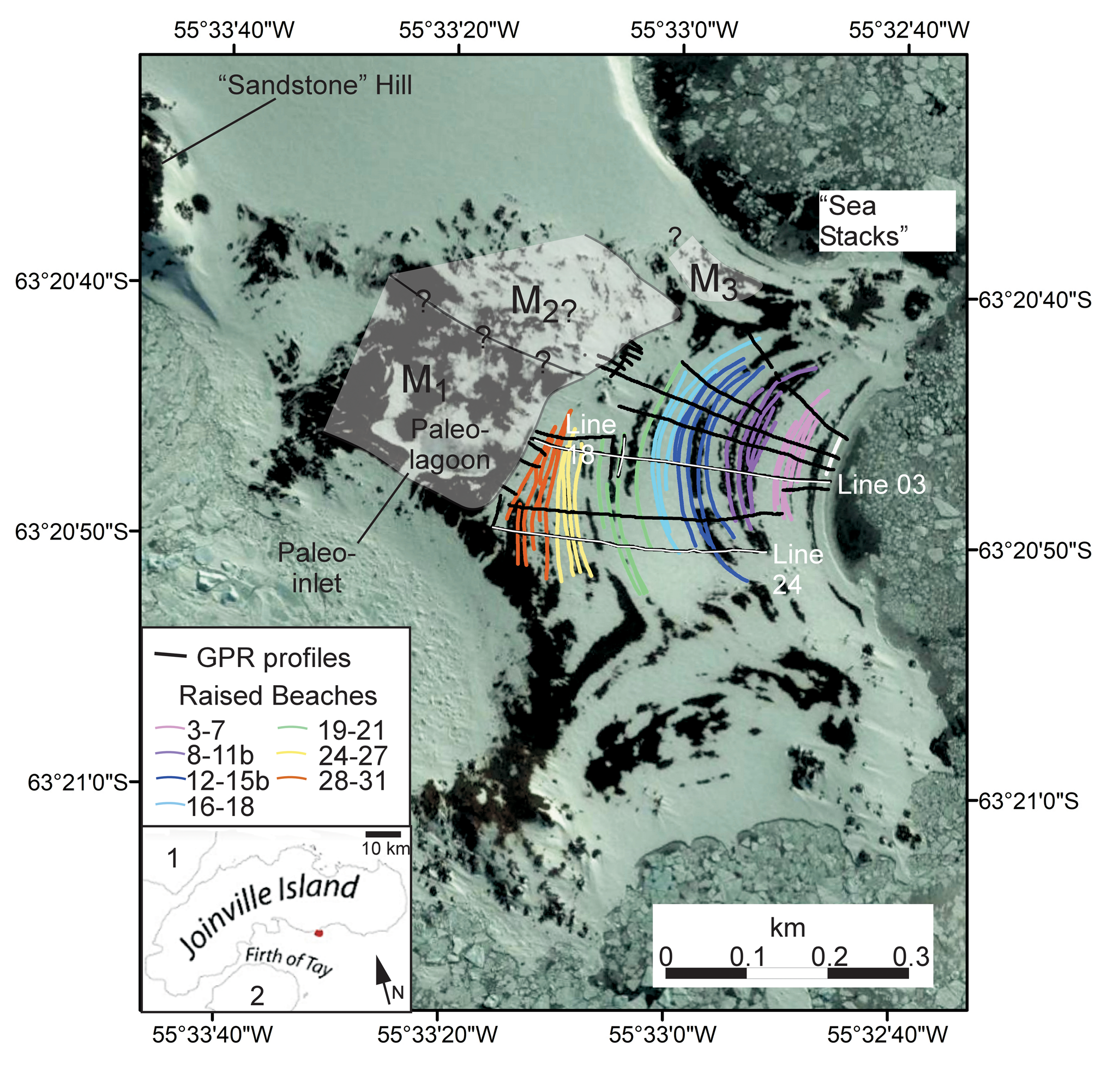
Fig. 2. Google Earth image of Tay Head on Joinville Island and the locations of the beaches, moraines (translucent grey) and ground-penetrating radar (GPR) profiles discussed in the text. Beaches 22 and 23 are not displayed because GPS data could not be processed. Inset map shows the location of Tay Head (red dot) on Joinville Island as well as the location of D'Urville Island (1) and Dundee Island (2).
The 36 discrete raised beach ridges (separated from one another by troughs) observed on Joinville Island are ~0.4 km long (shore parallel) and located on the east side of Tay Head, an ~2.0 km × 2.5 km peninsula positioned on the south side of Joinville Island (Fig. 2). A similar, more weakly developed series of beach ridges is found on the south-facing portions of Tay Head but were not surveyed. The field site is adjacent to the Firth of Tay, 15 km from the location of a SHALDRIL core from which Michalchuk et al. (Reference Michalchuk, Anderson, Wellner, Manley, Majewski and Bohaty2009) obtained a high-resolution record of Holocene deglacial and climate history.
Methods
Granulometry
The size and roundness of the largest 100 surface clasts within 1 m2 were observed, recorded and photographed, similar to the approaches of Simkins et al. (Reference Simkins, Simms and DeWitt2015) and Bentley et al. (Reference Bentley, Hodgson, Smith and Cox2005). This process was repeated three times along each crest of the 36 raised beaches. Clasts from the field and in photographs were classified into six categories: well rounded, rounded, sub-rounded, subangular, angular and very angular (Powers Reference Powers1953). Grain size was measured according to the two visible axes observed in photographs. Standard deviation was used to quantify sorting.
Out-of-place pebbles
The density of out-of-place pebbles (OPPs), identified as rock types not represented in the local bedrock or till outcrops, within a 15 m3 area on the crest of each beach (Fig. 3c) was measured along every other beach to aid in the reconstruction of glacial activity and provenance. These OPPs were generally interpreted as IRD; however, we cannot conclusively rule out their original transportation by an earlier (Last Glacial Maximum?) ice sheet that covered the whole region and later reworking into the beach deposits. In addition to what appeared to be exotic OPP clasts, we also counted the number of clasts of a distinctive rhyolite found in dikes within the local bedrock and sandstone (quartzite) clasts that appeared to be sourced from a local hill to the north-west of the beaches ('Sandstone Hill'; Figs 2 & 3d). However, we are less confident in our counting of the sandstone clasts compared to the rhyolite clasts due to the similarity of the sandstone and other local finer-grained metasedimentary bedrock. The difficulty of counting was exacerbated by snow cover at the time (Fig. 3c).
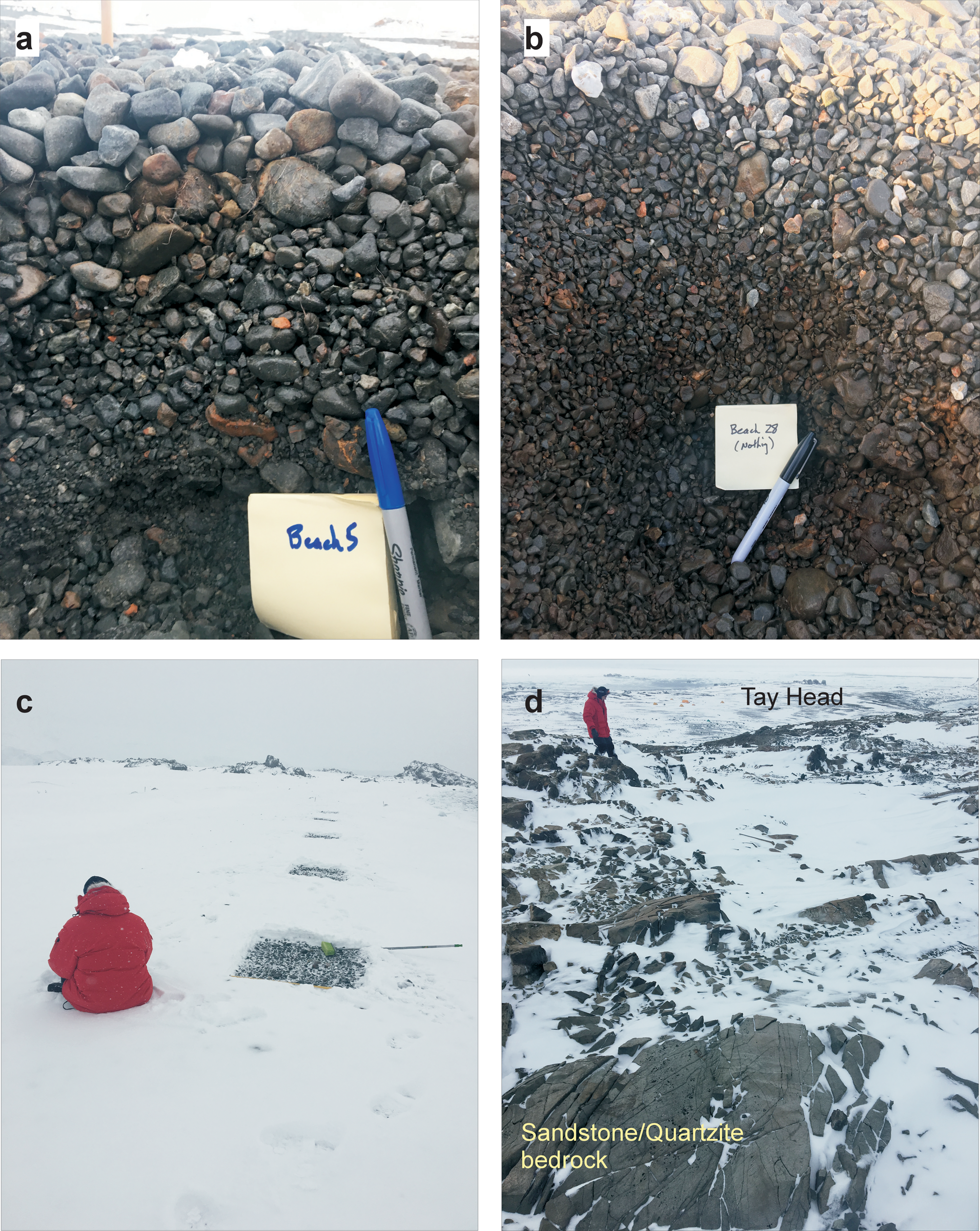
Fig. 3. Photographs of the field site including a. fabric of beach 5 deposits with well-bedded gravels and sands, b. fabric of beach 28 deposits lacking bedding and sands, c. snow cover and 1 m2 ‘pits’ in which out-of-place pebbles were counted and d. sandstone outcrop on the hill.
GPS and tide gauge
Joinville Island GPS and tide data are reported in Zurbuchen & Simms (Reference Zurbuchen and Simms2019). Elevation and coordinate data were obtained using a UNAVCO Trimble Net R9 receiver global navigation satellite system (GNSS) base station and Trimble 5700 GPS/GNSS receiver. Upon failure of the local base station, the O'Higgins permanent GPS station (www.sonel.org, last accessed 10 February 2023), located ~115 km away from Joinville Island, was used instead. Beach-ridge profiles were obtained from kinematic-mode GPS surveys across the crest of each beach ridge, except for beach ridges 2 and 3, which each have three static elevation points due to the presence of wildlife. GPS data were processed in Trimble Business Center with horizontal and vertical precisions of ~0.25 m. Elevations were converted to mean sea level using 2 days of data from a locally deployed Valeport 740 Portable Water Level Recorder (tide gauge) matched to the tide gauge at Bahia Esperanza ~50 km away.
Ground-penetrating radar
Approximately 2.5 km of GPR profiles were collected across the beaches of Tay Head using a Sensors and Software pulseEkko Pro with a 200 MHz antenna (Fig. 2; Zurbuchen & Simms Reference Zurbuchen and Simms2019). Lines were predominantly collected shore-normal, with four additional shore-parallel profiles collected to help tie the other profiles together. The unshielded antenna was mounted on a custom-built cart and manually pulled across the beaches. Processing of the GPR profiles included a topographic correction, DeWow (a proprietary processing algorithm) and a depth-varying gain, all conducted using EkkoDeluxe and Kingdom Suite software. A velocity of 0.190 m/ns was used based on a common midpoint survey conducted at the site.
Beach age
Beach-ridge ages on Joinville Island were estimated using previously published radiocarbon ages in addition to 18 new optically stimulated luminescence (OSL) age determination attempts. Zurbuchen & Simms (Reference Zurbuchen and Simms2019) obtained radiocarbon ages for 18 of the lower 21 beach deposits (labelled 0–18, including 7a, 7b, 15a, 15b) on Joinville Island. With the exception of the ages from beaches 1 and 2, which calibrate to < 448 years, these ages were recalibrated using Calib 8.2 (Heaton et al. Reference Heaton, Kohler, Butzin, Bard, Reimer and Austin2020), with an updated marine radiocarbon reservoir offset (Delta R) of 695 ± 140 (Hall et al. Reference Hall2010b; Calib.org/marine/regionalcalc.php, last accessed 16 August 2023). For the ages of beaches 1 and 2, we retained the ages originally used by Zurbuchen & Simms (Reference Zurbuchen and Simms2019), which were derived using a Bayesian progradation model for the beach-ridge age assignments. All ages in this study are given in calibrated years or thousands of years before present (the present being 1950). We use the notation ‘cal. yr BP’ to denote specific calibrated radiocarbon ages and ‘ka’ to represent time periods in the past and ‘OSL ages’ or ‘kyr’ for a span of time.
In order to supplement the previously reported radiocarbon ages by Zurbuchen & Simms (Reference Zurbuchen and Simms2019; https://doi.org/10.1130/2019370, last accessed 15 December 2022), cobbles and sands were sampled under lightproof conditions for OSL dating. We focused our efforts on the upper non-organic-bearing beaches. Sample preparation and OSL dating methods followed Simkins et al. (Reference Simkins, DeWitt, Simms, Briggs and Shapiro2016). The top, light-exposed portions were crushed for dose rate estimates. From the lower, light-shielded part of the cobble, the outer 1 mm surface was removed following Simms et al. (Reference Simms, DeWitt, Kouremenos and Drewry2011), who demonstrated that this layer was reset completely after 1 h of daylight exposure. The target slices were crushed by hand using a mortar and pestle in order to avoid pressures that could erase the luminescence signal. The carefully ground cobble grains and sediment from additional sandy deposits were prepared according to the following procedures: the material was sieved for grain sizes 63–250 μm. The grains were then washed in 10% HCl and 27% H2O2 to remove carbonate and organic material contaminates. The remaining sediment from sand and cobble samples was density separated with lithium polytungstate liquid (LST) at specific gravities of 2.75, 2.62, 2.58 and 2.54 to isolate quartz, potassium and sodium feldspars and heavy and light grains. The heavy and light grains were saved and stored away, whereas the remaining quartz and feldspar grains were etched using hydrofluoric acid (48% HF for 40 min for quartz and 10% HF for 15 min for feldspars). Some samples had only little material in the feldspar fraction. For those samples, it was not possible to separate sodium and potassium feldspars. These samples were treated as ‘mixed’ feldspars.
Measurements were conducted using a Risø TL/OSL-DA-20 reader, Risø National Laboratory, with a bialkali photomultiplier tube (Thorn EMI 9635QB). The built-in 90Sr/90Y beta source gives a dose rate of ~100 mGy/s. The exact dose rate value was calculated for the specific day on which each sample was measured. For quartz, optical stimulation was carried out with a blue LED array at 470 nm with 74 mW/cm2 (90%) power at the sample and a 7.5 mm Hoya U-340 detection filter (290–370 nm). Feldspars were stimulated with an infrared LED array at 870 nm with 121 mW/cm2 (90%) power at the sample and a blue or yellow filter combination for detection. The heating rate used was 5°C/s. Quartz grains did not have any significant luminescence signals. The measurement procedure for feldspar was based on the single-aliquot regenerative-dose (SAR) procedure described by Murray & Wintle (Reference Murray and Wintle2000) and Wintle & Murray (Reference Wintle and Murray2006). The procedure was modified such that the same temperature and 60 s duration were used for cutheat and preheat steps (compare Blair et al. Reference Blair, Kalchgruber and McKeever2007). The preheat temperatures were determined for each sample with plateau and dose recovery tests. The equivalent dose D e was determined with the central age model (Galbraith Reference Galbraith, Roberts, Laslet, Yoshida and Olley1999).
Calculation of the dose rate followed the procedure described in detail by Simms et al. (Reference Simms, DeWitt, Kouremenos and Drewry2011). Concentrations of natural uranium, 232Th and potassium were measured with high-resolution gamma-spectrometry for both rocks and surrounding material. All samples were in radioactive equilibrium. The water content for rocks was assumed to be 0. The water content for the surrounding materials was measured and has an uncertainty of 3%. Alpha, beta and gamma dose rates were calculated using the conversion factors published by Guérin et al. (Reference Guérin, Mercier and Adamiec2011). The internal K concentrations in the feldspar samples (for single grains as well as average values) were measured with an electron probe micro-analyser (EPMA) at the University of California, Santa Barbara. To calculate the resulting internal dose rates, the grain sizes of the feldspars in the rock samples were measured. The cosmic dose rate was calculated as described by Barbouti & Rastin (Reference Barbouti and Rastin1983), Prescott & Stephan (Reference Prescott and Stephan1982) and Prescott & Hutton (Reference Prescott and Hutton1994). The effective thickness was assumed to be half the burial depth. The uncertainty was 5%. Feldspar ages were fading corrected as described by Auclair et al. (Reference Auclair, Lamothe and Huot2003) and Wallinga et al. (Reference Wallinga, Bos, Dorenbos, Murray and Schokker2007) for the linear and non-linear dose ranges, respectively.
Results
Beach-ridge architecture
Beach ridges appear to naturally clump into beach-ridge sets based on similar elevations, with what appear to be natural breaks between groups of three to seven beach ridges (Fig. 4). The lower beach-ridge sets include beaches 1–7 (GPR profiles reveal another break between beaches 2 and 3), 8–11b, 12–15b and 16–18. Above beach ridge ~20, the beach ridges became less continuous and more difficult to correlate across the beach plain. Nevertheless, natural breaks appeared to continue into the upper beach ridges, with more weakly developed breaks between beach-ridge sets defined by beach ridges 19–23, 24–27 and 28–31 (Fig. 2). The slope in the beach-ridge plain also changes at beach ~15b (Fig. 5). Along the profile of GPR line 3, orientated perpendicular to the beach ridges, above beach ridge 15b the slope is ~0.056, whereas below that it is ~0.033. The decrease is greater along GPR line 24, for which above beach ridge 15b the slope is ~0.033, whereas below that it is ~0.015.

Fig. 4. Elevation transects across the crest of the most prominent beach ridges on Joinville Island. The 95% confidence intervals are shown by grey boxes. Not shown are beach ridges 2 and 3 due to limitations from local wildlife and beach ridges 21–23, whose GPS-processing error bars were so large as to obscure any meaningful results.
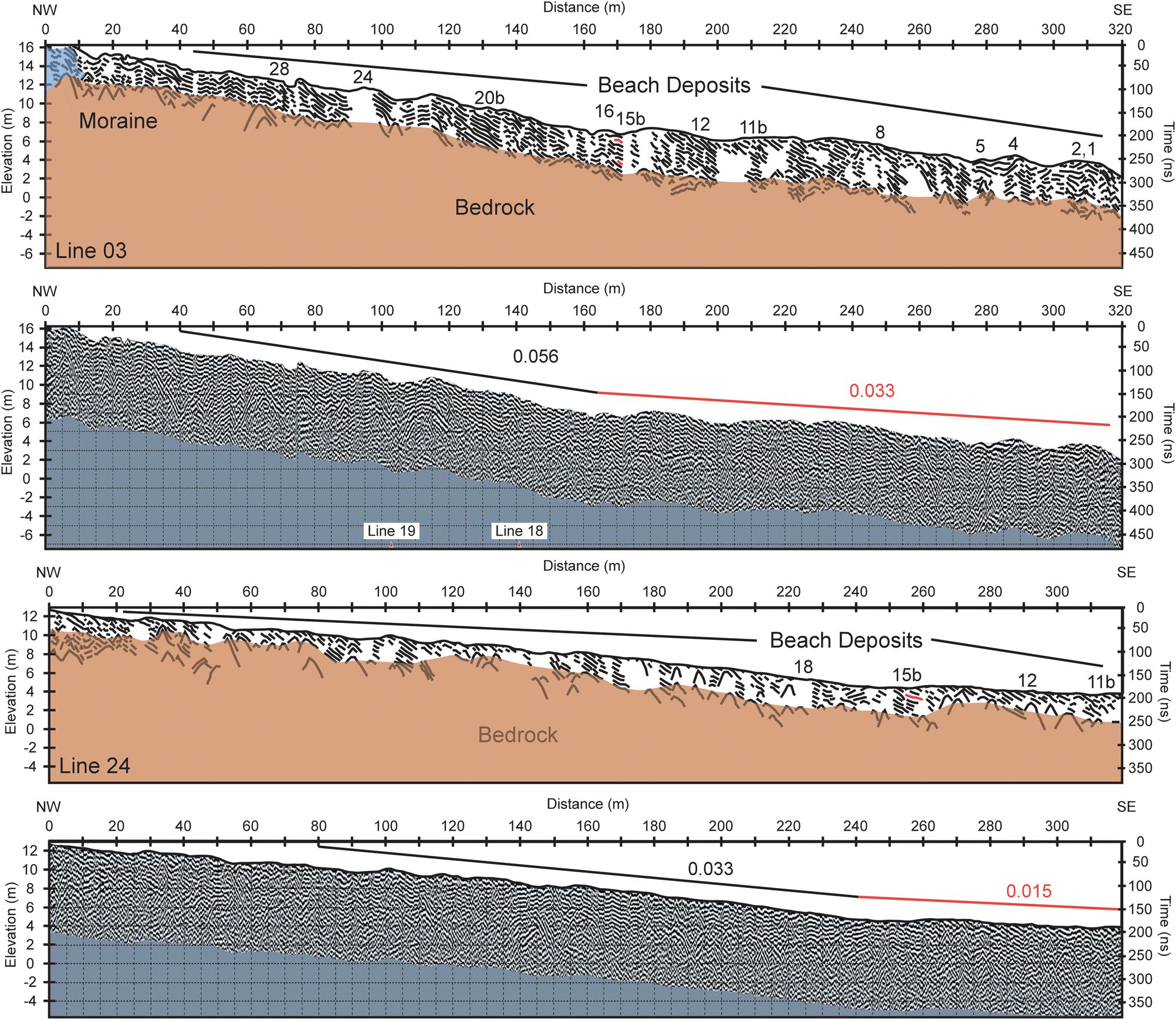
Fig. 5. Ground-penetrating radar (GPR) profiles and their interpretations for GPR lines 3 (upper two panels) and 24 (lower two panels). See Fig. 2 for GPR line locations.
Relationship between beaches and moraines
To the north of the raised beaches on Tay Head lie two to three moraines (Fig. 2; Simms et al. Reference Simms, Bentley, Simkins, Zurbuchen, Reynolds, DeWitt and Thomas2021). The oldest, M1, is located at the top (north-west) of the flight of raised beaches. M1 appears to be onlapped or at least coeval with the highest beach ridges. Its well-rounded cobbles and smooth outer margin suggest reworking by marine processes, possibly into a palaeo-spit. Its interior may have been occupied by a palaeo-lagoon, which today occasionally fills with an ephemeral pond, complete with a palaeo-tidal inlet (Fig. 6). However, the palaeo-lagoon only contains coarse, angular cobbles with little to no mud.
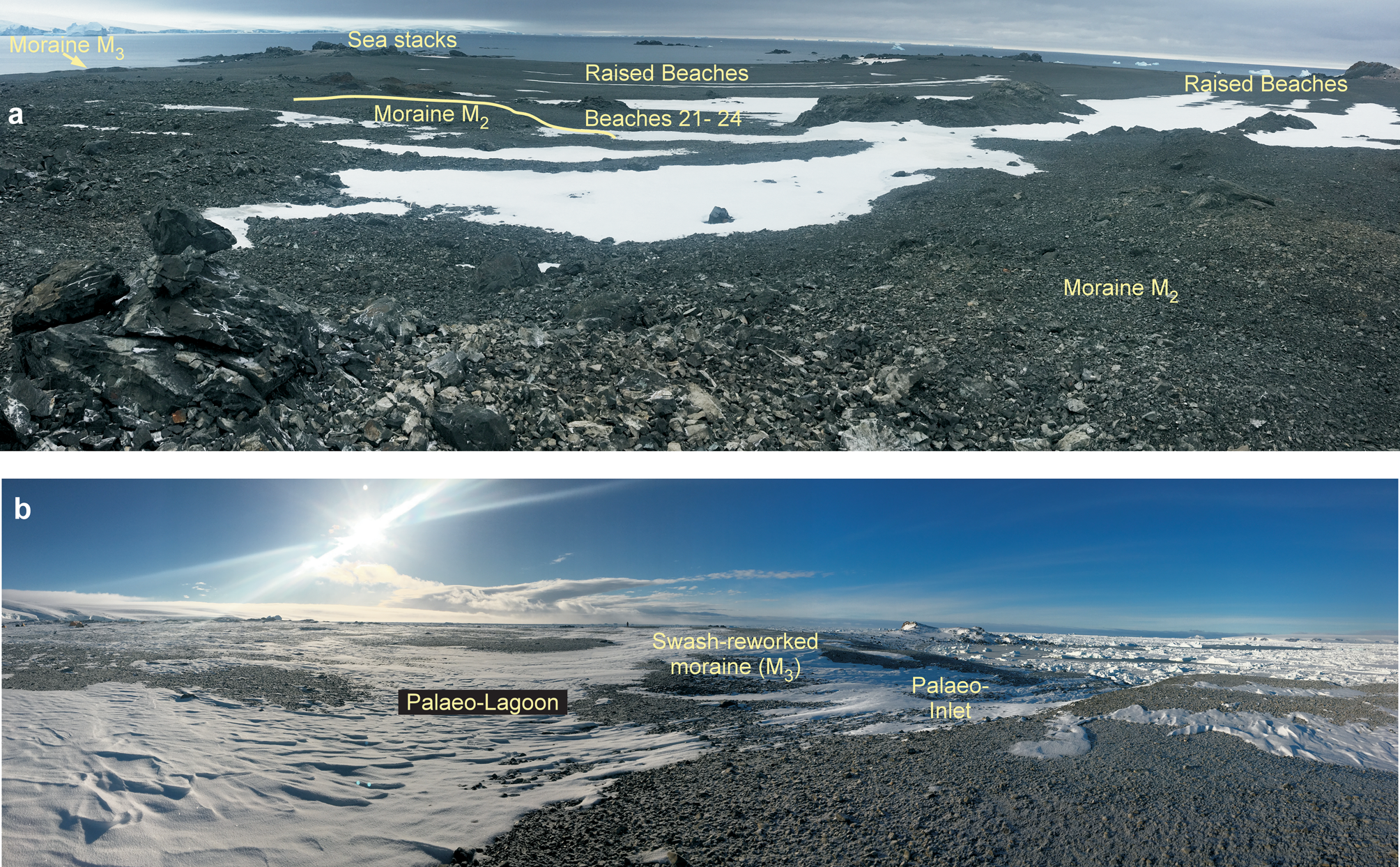
Fig. 6. a. Photograph looking east across Tay Head showing the relationship between the moraines and beaches as well as the character of M2. b. Photograph looking south-east into moraine M3 and the possible palaeo-lagoon formed within it as it was reworked by swash processes.
To the north-east of M1 lies another moraine or till sheet (M2). It appears younger than M1, as M2's southern margin overrides some of the younger raised beaches (beaches 21–24; Fig. 6). The surface of M2 is also hummocky (Fig. 6). Due to snow cover, the boundary between M1 and M2 was not clearly defined in the field, but it appears M2 overlies M1. To the east of M2 lies a third, younger moraine (M3) described by Simms et al. (Reference Simms, Bentley, Simkins, Zurbuchen, Reynolds, DeWitt and Thomas2021). M3 appears to be younger than M2, as beaches 19 and 17 are cross-cut by M3 but not clearly by M2. In addition, the cobbles within M2 are much more angular compared to the more rounded cobbles of M3, which probably reworked older beach deposits (Simms et al. Reference Simms, Bentley, Simkins, Zurbuchen, Reynolds, DeWitt and Thomas2021).
Beach sedimentary characteristics
Based on 9092 grain-size measurements, the pebbles within Joinville Island's 36 beaches average between 2 and 4 cm in maximum length, with an overall standard deviation of 1.11 cm (Fig. 7 & Table I). Fine grains (e.g. diameters < 2 mm) were almost absent within the upper 15 cm of the beach deposits (Fig. 3). The mean grain size and sorting of pebbles on Joinville Island beaches did not change by > 1 cm across all of the beaches (Fig. 7). The oldest (19–31) and the youngest (modern-6) beaches contain some of the coarsest material and also vary considerably from the beaches adjacent to them. The middle beaches (7–18) are slightly finer-grained, with less intra-beach variability. In addition, the sedimentary characteristics differed between the upper and lower beach deposits. The deposits of the lower 21 beaches (beach numbers 1–18, including 7b, 11b and the modern beach) were stratified with mats of seaweed within their matrix, whereas the deposits of the upper 15 beaches (beach numbers 19+) were not stratified and lacked seaweed (Fig. 3). Large, out-of-place (ice-rafted?) boulders also only occurred above beach ridge 20.
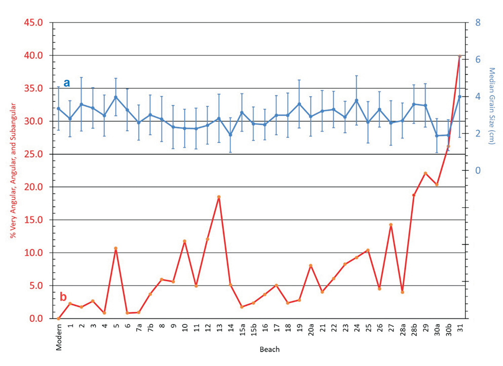
Fig. 7. a. Median long-axis grain size and b. the sum of the percentage of very angular, angular and subangular cobbles of the raised beaches at Tay Head, Joinville Island.
Table I. Granulometric characteristics of the raised beaches of Joinville Island.
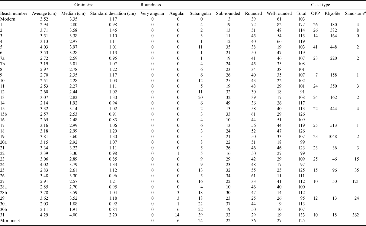
a Probably an underestimate (see text).
OPP = out-of-place pebble.
Roundness measurements performed on 4025 pebbles indicate the lower Joinville Island beaches are more rounded than the upper beaches (Fig. 7). Coarser grains are more easily rounded than finer grain sizes (cf. Boggs Reference Boggs2006), which could bias the roundness trends. However, after performing a permutation test on the data, the results failed to reject the null hypothesis of no correlation (Fig. S1), indicating grain size does not have an effect on the grain roundness of the Joinville Island beach deposits. Of the 36 beach deposits, nine modes are well rounded, 24 modes are rounded, two modes are sub-rounded and one mode is subangular (Table I). The general increase in pebble roundness through time is interrupted at beaches 5, 15, 16 and 28a (Fig. 7). Beach 5 exhibits less and beach 28a exhibits more rounding than the general trend (Fig. 7). Beach 5 is also one of the more coarse-grained beaches. The transition from beaches 15 to 14 indicates a decrease in pebble roundness over time, in opposition to the overall roundness trend.
The less-rounded deposits of beach 5 also have the most OPPs of any Joinville Island beach, whereas beach 9 has fewer OPPs than the surrounding beaches, and no changes in OPPs are seen through the transition from beaches 15 to 13 (Fig. 8). Unfortunately, OPP data were not directly counted for beach 28. In addition, the prevalence of more locally sourced rocks appears to change through time. Two of the most readily identifiable locally derived rock types observed while counting OPPs on Joinville Island were a low-silica rhyolite and sandstone/quartzite. Beaches 1–19 contained more low-silica rhyolite clasts, whereas beaches 21–31 contained less rhyolite and beaches 23–31 contained more sandstone clasts (Fig. 8).
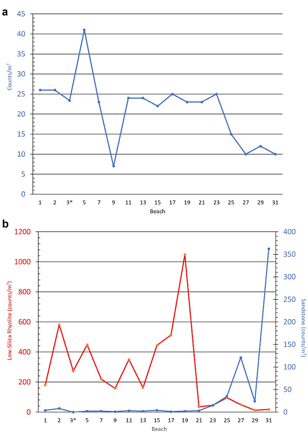
Fig. 8. a. Number of out-of-place pebbles (OPPs), interpreted as representing ice-rafted debris, per 1 m2 of the beach for selected beaches on Tay Head, Joinville Island. Pebble counts were collected within 15 m2 along the central portion of every other beach. b. Number of low-silica rhyolite (red) and sandstone (blue) pebbles per 1 m2 of beach counted in the same manner as the OPP. *Pebbles were only counted on 9 m2 of beach 3, thus the numbers presented have been normalized to 15 m2. Note the frequency of sandstone pebbles is probably an underestimate (see text).
Ground-penetrating radar survey results
The GPR profiles generally illustrate two dominant facies in the dip profiles. GPR facies #1 is composed of seaward-dipping, relatively continuous and parallel reflections (Fig. 9). In strike profiles, these regions are marked by flat-lying reflections (Fig. 10). GPR facies #2 is composed of chaotic, non-continuous, non-parallel reflections. Although hyperbolas are frequent throughout the data, they are most common at the interface between the two GPR facies and within GPR facies #2 (Fig. 10).
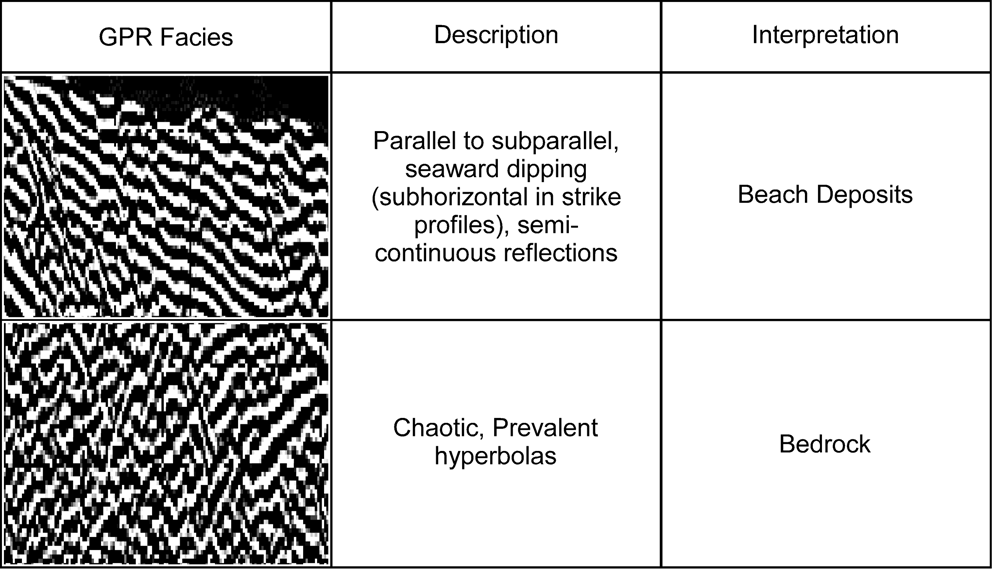
Fig. 9. Examples, descriptions and interpretations of ground-penetrating radar (GPR) facies #1 and #2.
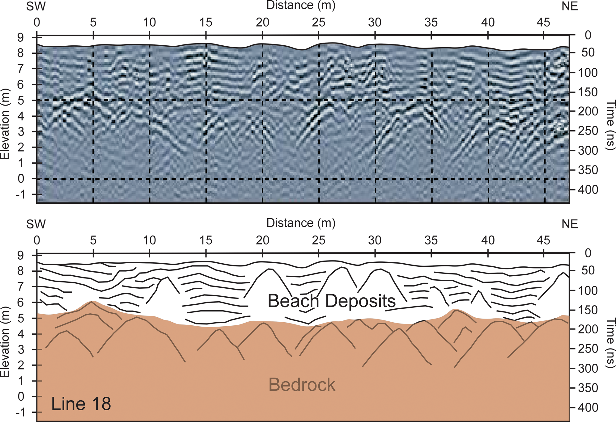
Fig. 10. Ground-penetrating radar (GPR) profile 8 and its interpretation. See Fig. 2 for the GPR line location.
Onlap is common within reflections of GPR facies #1 and is most common along the boundary between sets of beach ridges (e.g. between beaches 2 and 3, 5 and 6, 7 and 8, 11b and 12, around 22, between 27 and 28, and 29 and 30). One of the most prominent areas of onlap corresponds with an overall change in the slope of the overall beach-ridge plain between beach ridges 15b and 18 (red reflection tracings in Fig. 5). At this location, the slope of the beach-ridge plain increases updip (Fig. 5).
Beach ages
Radiocarbon ages for the lower Joinville Island beaches were produced from shell and seaweed materials interbedded within the beach deposits, and the recalibrated ages range from 105 ± 160 (beach 1) to 3190 ± 375 cal. yr BP (beach 18), varying by < 100 years from their original calibration reported in Zurbuchen & Simms (Reference Zurbuchen and Simms2019; Fig. 11; https://doi.org/10.1130/2019370, last accessed 15 December 2022). OSL ages range from modern to ~68.3 ± 17 ka (see the ‘Discussion’ section below). A summary of the samples and OSL ages is listed in Table II. Detailed results can be found in the Supplemental Materials (Tables S1 & S2). Out of 13 sediment samples, only seven had grain sizes in the range suited for OSL dating, whereas the others were too coarse. While 22 cobble surface samples were prepared, eight samples had no luminescence signal at all, even after irradiation with 100 Gy. Sand samples had generally brighter signals than cobble samples. Exceptions were the K-feldspar fractions of JV-26 and JV-32 (~106 cps after 10 Gy irradiation). Dose recovery tests ranged from very good (> 5%) to medium (> 10%). The large overdispersion values (Table S2) are probably caused by the necessary crushing of the slices. Large grains with dose gradients inside the grain are broken into multiple pieces. Breakage inside grains instead of at grain boundaries leads to grains that consist of mineral mixtures. This is evidenced by the fact that grains in the Na-feldspar fraction were found to have comparatively high internal K concentrations (compare, for example, JV-27; Table S1). Fading rates had large measurement uncertainties due to the low signals and large differences between different aliquots of the same sample.
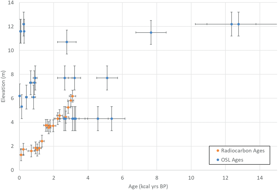
Fig. 11. Graph illustrating the height and age of beaches dated using optically stimulated luminescence (OSL) and radiocarbon dating.
Table II. Optically stimulated luminescence ages and sample properties.
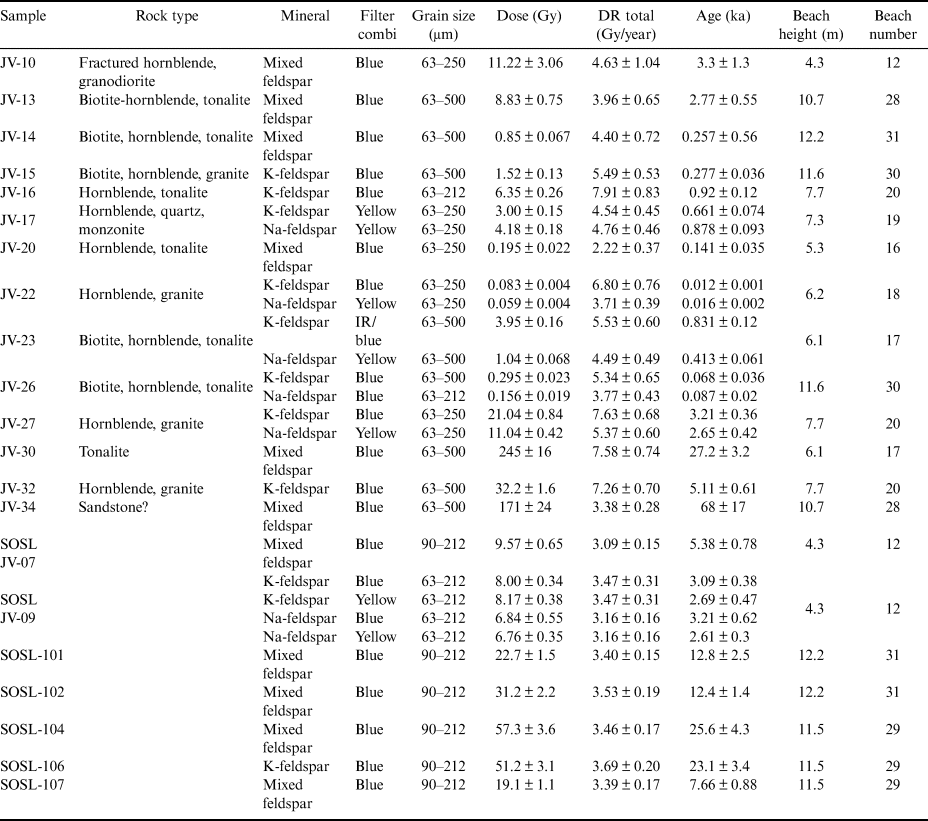
All samples labelled ‘JV-x’ are rock samples. Samples labelled SOSL-x are sediment samples.
Minerals: for samples with sufficient materials, feldspars were separated into K-feldspar (< 2.58 SG) and Na-feldspar (> 2.58 SG). For all other samples, the fraction < 2.62 SG was labelled as ‘mixed’ feldspars.
Filter combi: in general, the brightest signal was used for dating. For most mixed feldspars and K-feldspars this was the blue signal, whereas Na-feldspars were brighter in yellow. There are some exceptions, as listed.
Grain size: the grain size was obtained after sifting of sediments or after crushing and sifting of rock slices.
Age: the final age, after fading correction where applicable.
Beach height: the height of the beach in metres where the sample was collected.
DR = dose rate; IR = infrared.
Discussion
Optically stimulated luminescence ages vs radiocarbon ages
Even when considering the challenging properties of the OSL samples, it is not fully clear why such a large discrepancy exists between the radiocarbon and OSL ages. We favour the radiocarbon ages over the OSL ages given their self-consistency (e.g. higher beach ridges return older ages and multiple ages from the same beach ridge are within error of one another) and agreement with regional records of RSL (e.g. Roberts et al. Reference Roberts, Hodgson, Sterken, Whitehouse, Verleyen and Vyverman2011). Some of the OSL samples (including JV17, JV27, JV32, SOSL JV-09 and SOSL-106) showed very good luminescence properties: very good dose recovery, low overdispersion values and small uncertainties for the fading rates. For some of the samples (JV17, JV27, SOSL JV-09), ages were measured with both K-Feldspar and Na-feldspar fractions, and the two independent results agree in each case within 1-sigma error limits. Yet the OSL ages show little to no agreement with the radiocarbon ages. Four beaches (beaches 12 and 16–18) were sampled by both OSL and radiocarbon dating. Of those, only OSL ages from beach ridge 12 fall within error of the radiocarbon ages (Fig. 11). All ages except one from beaches 16–18 returned anomalously young ages, possibly reflecting exposure after ridge formation. The other age is much older than expected (Table II). The ages from the higher beach ridges appear to suffer from similar uncertainties, with seven of the 17 ages dating to < 500 years old despite probably being older than 3 ka based on the radiocarbon ages. Similarly, three others are younger than ~3 ka, despite being higher than the 3 ka-old beaches based on the radiocarbon ages. Three more OSL ages are anomalously old at ~68, 27 and 25 ka and may reflect incomplete resetting during their last exposure. Two separate ages obtained from the same beach ridge date to an apparently anomalously old age of 12 ka, but they appear correct based on their OSL characteristics. Their age is intriguing but probably too old based on the glacial history of the region (Michalchuk et al. Reference Michalchuk, Anderson, Wellner, Manley, Majewski and Bohaty2009). That leaves two ages that fit the general RSL trend of the younger radiocarbon-based chronology: JV-32, with an age of 5.1 ± 0.6 ka from beach 20 at an elevation of 7.7 m, and SOSL-107, with an age of 7.7 ± 0.9 ka from beach 29 at an elevation of 11.5 m. Assuming an average rate of beach formation of 175 years, based on the frequency of the lower 14C-dated beaches, the age of beach 31 is expected to be older than 5.8 ka, and accounting for hiatuses would probably make the section older.
Neoglacial and beach architecture
Several shifts in beach characteristics are observed in the beaches of Tay Head, but the largest and most pronounced change occurs around beaches 15a and 15b. At this point, the slope of the larger beach plain decreases (Fig. 5), and it is near the onset of seaweed preservation and the development of well-defined stratification within the beaches (beach 18), although we cannot rule out the possibility that the change in fabric is due to post-depositional changes (e.g. frost processes) to the upper beach ridges. Adjacent beach ridge 15a also marks a significant interruption in the general increase in pebble roundness through time (Fig. 7). The age of beaches 15a and 15b (~2.7 ka) corresponds to the onset of the well-documented Neoglacial time period between ~2.1 and ~2.5 ka (Bentley et al. Reference Bentley, Hodgson, Smith, Cofaigh, Domack and Larter2009, Cejka et al. Reference Cejka, Nyvlt, Kopalova, Bulinova, Kavan and Lirio2020). Pronounced cooling on James Ross Island supports the onset of the Neoglacial period at 2.5 ka (Mulvaney et al. Reference Mulvaney, Abram, Hindmarsh, Arrowsmith, Fleet and Triest2012, Totten et al. Reference Totten, Anderson, Fernandez and Wellner2015, Kaplan et al. Reference Kaplan, Strelin, Schaefer, Peltier, Martini and Flores2020), although some proxies, such as those from a SHALDRIL core taken in the Firth of Tay (Michalchuk et al. Reference Michalchuk, Anderson, Wellner, Manley, Majewski and Bohaty2009) and the Palmer Deep Site 1098 on the western AP (Domack Reference Domack2002, Shevenell & Kennett Reference Shevenell and Kennett2002, Shevenell et al. Reference Shevenell, Ingalls, Domack and Kelly2011), suggest that the Neoglacial period initiated earlier, at closer to 3.5 ka, whereas others along the EAP suggest the Neoglacial period to be younger (Cejka et al. Reference Cejka, Nyvlt, Kopalova, Bulinova, Kavan and Lirio2020). Along Tay Head, prolonged cooling associated with the Neoglacial time period could have increased sea-ice conditions and hindered clast rounding, leading to a decrease in pebble roundness, but this did not close the sea off enough to prevent icebergs from landing on the shore. Additionally, cooling may have driven localized glacier readvance (see below) and potentially increased sediment supply to the coast. An increased sediment supply could have led to the introduction of more angular beach clasts and a change in shoreline trajectory, leading to the lower slopes of the beach plain.
Other changes in Joinville Island beaches and their pebble roundness
In addition to the major change centred around beach ridge 15b at 2.7 ka, beach sets on Tay Head show breaks within the last ~0.7 kyr (the break between beaches 2 and 3), ~1.4 ka (beaches 7 and 8), ~2.1 ka (beaches 11b and 12) and sometime after ~3.2 ka with the age of the older breaks above beach 18, with the exception of the break between beaches 27 and 28 at ~7.5 ka, being poorly constrained. The younger events appear to coincide with glacial advances on the western AP documented by overridden mosses at ~0.2, ~0.8 and ~1.2 ka (Groff et al. Reference Groff, Beilman, Yu, Ford and Xia2023). Zurbuchen & Simms (Reference Zurbuchen and Simms2019) suggest that the breaks at ~1.4 and ~2.1 ka were the result of increases in the rate of RSL fall due to glacial isostatic adjustment-driven uplift. The others may be driven by a similar process. Interestingly, the events at ~1.4 and ~2.7 ka correspond to Bond events #1 and #2 (Bond et al. Reference Bond, Heinrich, Broecker, Labeyrie, McManus and Andrews1992).
In addition to the large interruption in beach pebble roundness as a potential result of the Neoglacial, the overall increase in beach pebble roundness through time on Joinville Island was interrupted at beaches 5 and 28a (Fig. 7). These interruptions do not correlate with inferred RSL changes described by Zurbuchen & Simms (Reference Zurbuchen and Simms2019), which suggests that these differences were caused by factors other than changes in the rate of RSL. Beach 5 contains less rounded materials and formed 1005 ± 310 cal. yr BP. The formation of beach 5 corresponds in timing with a negative Southern Hemisphere Annular Mode (SAM) event, which marks cooler climate conditions as the southern westerlies probably shifted towards the equator (Kwok & Comiso Reference Kwok and Comiso2002, Moreno et al. Reference Moreno, Vilanova, Villa-Martínez, Dunbar, Mucciarone and Kaplan2018, Kaplan et al. Reference Kaplan, Strelin, Schaefer, Peltier, Martini and Flores2020). The temperature anomaly record from the James Ross Island ice core (Mulvaney et al. Reference Mulvaney, Abram, Hindmarsh, Arrowsmith, Fleet and Triest2012) supports this suggestion, as temperatures were low at the time and continued to decrease thereafter. Additionally, anomalously low pebble roundness values are also found in Marguerite Bay (Simkins et al. Reference Simkins, Simms and DeWitt2015) at the same time as the formation of Joinville Island beach 5. Thus, the reduced rounding of sediments within beach 5 could be the result of a widespread period of less open water conditions, with an increase in sea ice observed in the relative abundance of diatom assemblages in other marine records (Barbara et al. Reference Barbara, Crosta, Leventer, Schmidt, Etourneau, Domack and Massé2016), indicative of cooler temperatures. Additionally, beach 5 has the highest OPP count, interpreted as representing IRD, which further supports the importance of cooler temperatures during the formation of beach 5. Cooler temperatures might have led to a glacial advance on Joinville Island and/or surrounding regions and supplied more icebergs carrying IRD (Bond et al. Reference Bond, Heinrich, Broecker, Labeyrie, McManus and Andrews1992). According to Mulvaney et al. (Reference Mulvaney, Abram, Hindmarsh, Arrowsmith, Fleet and Triest2012), a permanent ice shelf formed after ~1.5 ka within the Prince Gustav Channel, which offers a potential source of IRD for beach 5. Additionally, ice advances on James Ross Island (Björck et al. Reference Björck, Olsson, Ellis-Evans, Håkansson, Humlum and de Lirio1996, Kaplan et al. Reference Kaplan, Strelin, Schaefer, Peltier, Martini and Flores2020) and nearby islands (Balco & Schaefer Reference Balco and Schaefer2013) occurred at or after 1.4 ka.
Finally, beach 28a had more rounded beach materials compared to the overall roundness trend (Fig. 7). Increased pebble roundness could reflect higher wave exposure, suggestive of less sea-ice coverage. The second beach above beach 28a, beach 29, has an OSL age of 7.7 ± 0.9 ka. If the average rate of beach formation is ~175 years, then that would suggest an age of ~7.4 ka for beach 28. Marine records from the neighbouring Firth of Tay (Majewski & Anderson Reference Majewski and Anderson2009, Michalchuk et al. Reference Michalchuk, Anderson, Wellner, Manley, Majewski and Bohaty2009) suggest the onset of warmer and more open water conditions at about this time. At ~7.8 ka, Michalchuk et al. (Reference Michalchuk, Anderson, Wellner, Manley, Majewski and Bohaty2009) observed a distinct change in the marine sediments of the Firth of Tay, with an increase in diatoms, organic carbon, nitrogen and biogenic silica and a decrease in IRD. However, similar signals are not ubiquitous throughout the region (e.g. Shevenell et al. Reference Shevenell, Ingalls, Domack and Kelly2011, Mulvaney et al. Reference Mulvaney, Abram, Hindmarsh, Arrowsmith, Fleet and Triest2012, Barbara et al. Reference Barbara, Crosta, Leventer, Schmidt, Etourneau, Domack and Massé2016).
Joinville Island glacial advance
The increase in low-silica rhyolite and the decrease in sandstone clasts with time on the beaches of Tay Head could be manifestations of a change in beach sediment provenance. Outcrops of the sandstone are located west of the three moraines or till sheets, whereas the low-silica rhyolite was present as dikes within low-grade, metamorphosed, fine-grained sedimentary rocks in the sea stacks and outcrops on the eastern side of Tay Head (Fig. 2). The rocks within the westernmost M1 moraine behind beach 31 were dominantly sandstone. Therefore, the sediment sources for the upper beaches (21–31) were most probably the moraine and sandstone outcrops to the east, and, as beaches became preserved, eventually the sandstone sources were abandoned or swamped by materials from other parts of the peninsula. Subsequently, the dominant sediment source transitioned to the low-grade, metamorphosed, fine-grained sedimentary rocks with the low-silica rhyolite dykes for the lower beaches. However, this transition does not align with changes in pebble roundness, indicating that processes other than just a source change caused the changes in pebble roundness. Although the age of the westernmost moraine M3 is unknown, beach 31 cuts into the moraine, suggesting that it is older than 7.7 ka.
Two other moraines or till sheets are present north of the beaches on Tay Head (M2 and M3; Fig. 2). The sandstone would have been transported east by glacial ice to form the upper moraine (M1) and hence sourced the upper beaches (21–31). The low-silica rhyolite and its affiliated low-grade, metamorphosed, fine-grained sedimentary rocks are present in the area. The easternmost two moraines appeared to be composed of these rocks. The middle of the two moraines, M2, cuts across beaches 21–24, which we estimate to be 175–525 years older than beach 20, which has an OSL age of 5.1 ± 0.6 ka; whereas the lower moraine, M3, cuts across beaches 12 and possibly beach 8, thus post-dating ~1.5 ka BP as reported by Simms et al. (Reference Simms, Bentley, Simkins, Zurbuchen, Reynolds, DeWitt and Thomas2021). However, we cannot rule out the possibility that M2 and M3 represent the same advance but with a very irregular margin.
Conclusion
Changes in the sediment characteristics as revealed in GPR profiles, grain size, grain roundness and IRD within Holocene raised beaches on Joinville Island along the EAP were used to determine how the environmental history of the region is reflected within their deposits. A particularly well-developed set of 36 raised beaches is found on Tay Head on the southern side of Joinville Island. The lower 21 beaches are well stratified and better developed than the upper 15 beaches, which are unstratified and less contiguous. Furthermore, most beaches are found in sets of three to seven beach ridges separated from other beach-ridge sets by natural breaks in elevation without beach ridges. Grains on the raised beaches of Joinville Island show an overall increase in beach pebble roundness through time, whereas grain size shows no obvious pattern. However, the pebble roundness trend is interrupted at beaches 5, 15a and 28a. Beach 5 exhibits less and beach 28a exhibits more rounding than the general trend. The transition between beaches 15 and 14 indicates a sharp decrease in pebble roundness through time, in opposition to the overall pebble roundness trend. The change in roundness trend is also nearly concurrent with an inflection point in the overall slope of the beach plain and observable onlapping in GPR profiles. The lower 21 beaches contain prevalent seaweed mats and limpet shells, providing an excellent radiocarbon chronology. An attempt to date four of the lower radiocarbon-dated beaches and five of the upper beaches with 21 OSL ages from cobble surfaces as well as more traditional sand grains was met with mixed success. The age of beaches 15a and 15b (~2.7 ka), which marked a transition in pebble roundness of the beaches as well as a lowering of the overall beach plain slope, coincides with the onset of the Neoglacial time period of ~2.5–3.0 ka. Less rounding of sediments within the ~1.0 ka beach 5, which also had the most OPPs (interpreted as representing IRD) of any beach on Joinville Island, could be explained by a period marked by shorter open water seasons and an increase in sea ice, whereas the opposite could hold true for beach 28a of ~7.4 ka. This study suggests Holocene environmental changes left a measurable impact on the coastal zones of Antarctica.
Acknowledgements
We would like to thank Cara Ferrier and Laura Reynolds for their help in the field. We would also like to thank the captains and crews of the Lawrence M. Gould and Almirante Iraizar, without whose help we would still be on Joinville Island. Aidan Patterson helped with grain size and shape characterization. Gareth Seward performed EPMA measurements of feldspar separates. Claire Divola helped draft Fig. 4. We would also like to thank Daniel Nývlt and an anonymous reviewer for their constructive comments that helped improve the manuscript.
Financial support
This work was supported through National Science Foundation (NSF) grant 0724929 to ARS and RD. Additional support was provided by a Geological Society of America Graduate Student Research Grant and an NSF Graduate Research Fellowship to JZ.
Author contributions
ARS and RD designed the experiment. ARS, JZ and CGa conducted the fieldwork. ARS and JZ conducted the ground-penetrating radar analysis. BMT conducted the grain size and roundness analysis as well as the ice-rafted debris counting and initial interpretations. BMT, RD, CGa and CGe conducted the optically stimulated luminescence analysis. BMT and ARS wrote the manuscript with input from RW, CGe and the rest of the authors.
Supplementary materials
Two supplemental tables and a supplemental figure will be found at https://doi.org/10.1017/S0954102023000275.


 Open access