

I. INTRODUCTION
Recent progress in visual capture technology has enabled the capture and digitization of points corresponding to a 3D world scene. Point clouds are one of the major 3D data representations, which provide, in addition to spatial coordinates, attributes (e.g. color or reflectance) associated with the points in a 3D world. Point clouds in their raw format require a huge amount of memory for storage or bandwidth for transmission. For example, a typical dynamic point cloud used for entertainment purposes usually contains about 1 million points per frame, which at 30 frames per second amounts to a total bandwidth of 3.6 Gbps if left uncompressed. Furthermore, the emergence of higher resolution point cloud capture technology imposes, in turn, even a higher requirement on the size of point clouds. In order to make point clouds usable, compression is necessary.
The Moving Picture Expert Group (MPEG) has been producing internationally successful compression standards, such as MPEG-2 [Reference Tudor1], AVC [Reference Richardson2], and HEVC [Reference Sullivan, Ohm, Han and Wiegand3], for over three decades, many of which have been widely deployed in devices like televisions or smartphones. Standards are essential for the development of eco-systems for data exchange. In 2013, MPEG first considered the use of point clouds for immersive telepresence applications and conducted subsequent discussions on how to compress this type of data. With increased use cases of point clouds made available and presented, a Call for Proposals (CfP) was issued in 2017 [4]. Based on the responses made to this CfP, two distinct compression technologies were selected for the point cloud compression (PCC) standardization activities: video-based PCC (V-PCC) and geometry-based PCC (G-PCC). The two standards are planned to be ISO/IEC 23090-5 and -9, respectively.
The goal of this paper is to give an insight into the MPEG PCC activity. We describe also the overall codec architecture, its elements and functionalities, as well as the coding performance specific to various use cases. We also provide some examples that demonstrate the available flexibility on the encoder side for higher coding performance and differentiation using this new data format. The paper is presented as follows. Section II offers a generic definition for point cloud, along with use cases and a brief description of the current standardization activity. Section III describes the video-based approach for PCC, also known as V-PCC, with a discussion of encoder tools for PCC. In Section IV, there is a discussion of the geometry-based approach for PCC, or G-PCC, with the examples of encoding tools. Section V presents performance metrics for both approaches, and Section VI concludes the article.
II. POINT CLOUD
In this section, we define common terms for point clouds, present use cases, and discuss briefly the ongoing standardization process and activities.
A) Definition, acquisition, and rendering
A point cloud is composed of a collection of points in a 3D space. Each point in the 3D space is associated with a geometry position together with the associated attribute information (e.g. color, reflectance, etc.). The 3D coordinates of a point are usually represented by floating-point values; they can however be quantized into integer values according to a pre-defined space precision. The quantization process creates a grid in 3D space, and all the points residing within each sub-grid volume are mapped to the sub-grid center coordinates, referred to henceforth as voxels. This process of converting the floating-point spatial coordinates to grid-based coordinates representation is also known as voxelization. Each voxel can be considered a 3D extension of pixels corresponding to the 2D image grid coordinates. Notice that the space precision may affect the perceived quality of the point cloud, as shown in Fig. 1.
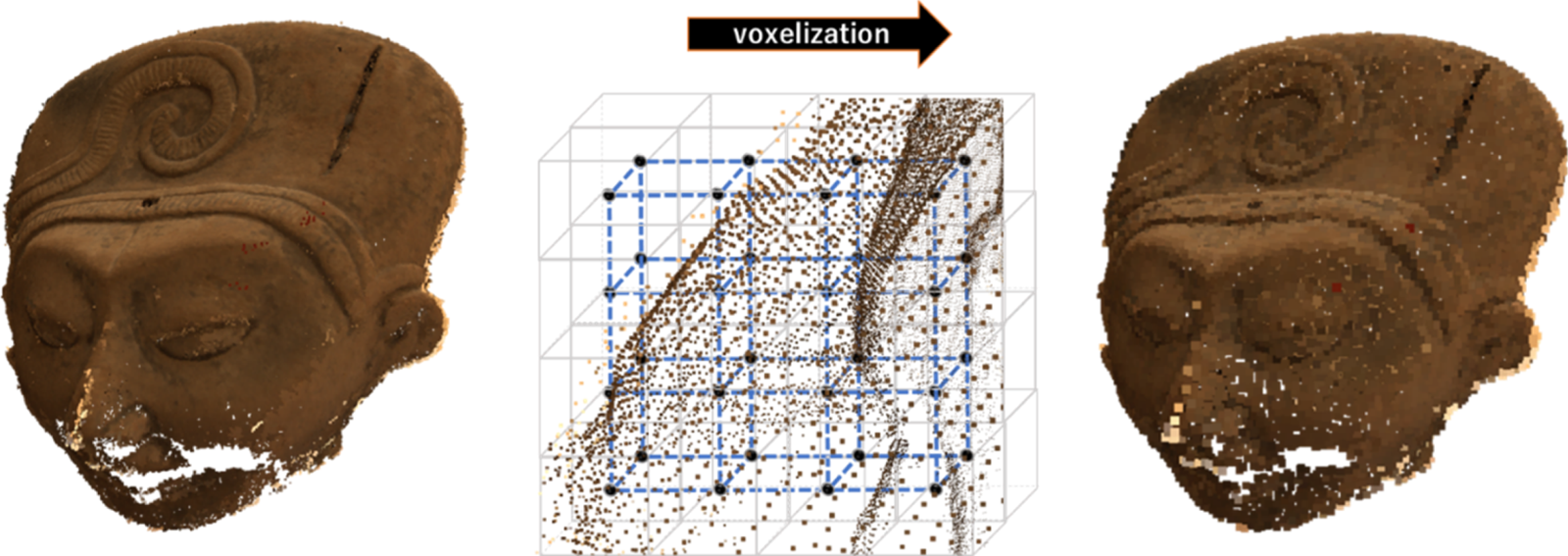
Fig. 1. Original point cloud with floating-point coordinates (left) and voxelized point cloud with integer coordinates (right).
The spatial information can be obtained using two different methods: passive or active. Passive methods use multiple cameras and perform image matching and spatial triangulation to infer the distance between the captured objects in 3D space and the cameras. Several variations of stereo matching algorithms [Reference Scharstein and Szeliski5] and multiview structure [Reference Kim, Kogure and Sohn6] have been proposed as passive methods for depth acquisition. Active methods use light sources (e.g. infra-red or lasers) and back-scattered reflected lights to measure the distances between the objects and the sensor. Examples of active depth sensors are Microsoft Kinect [Reference Zhang7], Apple TrueDepth Camera [8], Intel Realsense [9], Sony DepthSense [10], and many others.
Both active and passive depth acquisition methods can be used in a complementary manner to improve the generation of point clouds. The latest trend in capture technology is volumetric studios, where either passive methods (using RGB cameras only) or a combination of passive and active methods (using RGB and depth cameras) creates a high-quality point cloud. Examples of volumetric capture studios are 8i [11], Intel Studios [12], and Sony Innovation Studios [13].
Different applications can use the point cloud information to execute diverse tasks. In automotive applications, the spatial information may be used to prevent accidents, while in the entertainment industry application, the 3D coordinates provide an immersive experience to the user. For the entertainment use case, rendering systems based on point cloud information are also emerging, and solutions based on point cloud editing and rendering are already available (e.g. Nurulize [14] provides solutions for editing and visualization of volumetric data).
B) Use cases
There are accordingly many applications that use point clouds as the preferred data capture format. Here we explain some typical use cases, also shown in Fig. 2.
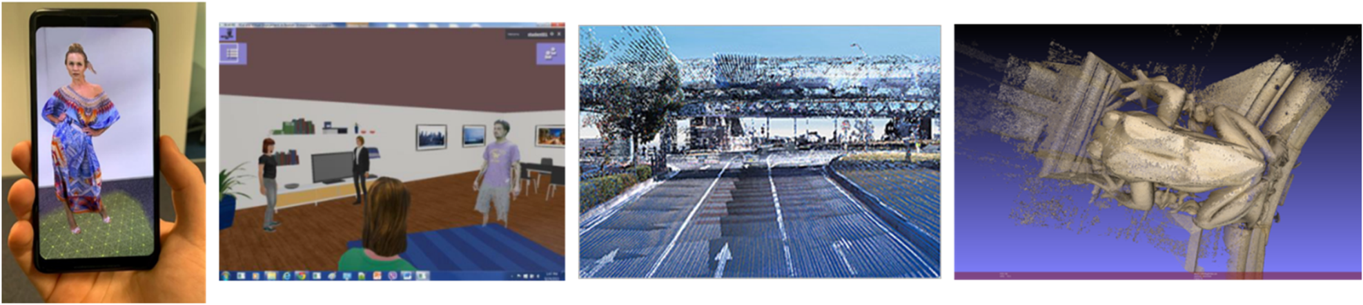
Fig. 2. Use case examples for point clouds, from left to right: VR/AR [Reference Chou15], Telepresence [16], autonomous vehicles [Reference Flynn and Lasserre17], and world heritage [Reference Tulvan and Preda18].
1) VR/AR
Dynamic point cloud sequences, such as the ones presented in [Reference Chou15], can provide the user with the capability to see moving content from any viewpoint: a feature that is also referred to as 6 Degrees of Freedom (6DoF). Such content is often used in virtual/augmented reality (VR/AR) applications. For example, in [Reference Schwarz and Personen19, Reference Ricard, Guillerm, Olivier, Guede and Llach20], point cloud visualization applications using mobile devices were presented. Accordingly, by utilizing the available video decoder and GPU resources present in a mobile phone, V-PCC encoded point clouds were decoded and reconstructed in real-time. Subsequently, when combined with an AR framework (e.g. ARCore, ARkit), the point cloud sequence can be overlaid on a real world through a mobile device.
2) Telecommunication
Because of high compression efficiency, V-PCC enables the transmission of a point cloud video over a band-limited network. It can thus be used for tele-presence applications [16]. For example, a user wearing a head mount display device will be able to interact with the virtual world remotely by sending/receiving point clouds encoded with V-PCC.
3) Autonomous vehicle
Autonomous driving vehicles use point clouds to collect information about the surrounding environment to avoid collisions. Nowadays, to acquire 3D information, multiple visual sensors are mounted on the vehicles. LIDAR sensor is one such example: it captures the surrounding environment as a time-varying sparse point cloud sequence [Reference Flynn and Lasserre17]. G-PCC can compress this sparse sequence and therefore help to improve the dataflow inside the vehicle with a light and efficient algorithm.
4) World heritage
For a cultural heritage archive, an object is scanned with a 3D sensor into a high-resolution static point cloud [Reference Tulvan and Preda18]. Many academic/research projects generate high-quality point clouds of historical architecture or objects to preserve them and create digital copies for a virtual world. Laser range scanner [Reference Curless and Levoy21] or Structure from Motion (SfM) [Reference Ullman22] techniques are employed in the content generation process. Additionally, G-PCC can be used to lossless compress the generated point clouds, reducing the storage requirements while preserving the accurate measurements.
C) MPEG standardization
Immersive telepresence was the first use case of point clouds that was discussed by MPEG back in 2013. The dynamic nature of points, distributed irregularly in space, tends to generate large amounts of data and thus provided initial evidence of the need for compression. Due to an increased interest from the industry on point clouds, MPEG collected requirements [23] and started the PCC standardization with a CfP [4] in January 2017. Three main categories of point cloud content were identified: static surfaces (category 1), dynamic surfaces (category 2), and dynamically-acquired LIDAR sequences (category 3). After the CfP was issued, several companies responded to the call with different compression technology proposals. At first, MPEG identified three distinct technologies: LIDAR point cloud compression (L-PCC) for dynamically acquired data, surface PCC (S-PCC) for static point cloud data, and V-PCC for dynamic content [Reference Schwarz S.24]. Due to similarities between S-PCC and L-PCC, the two proposals were later merged together into and referred to as G-PCC. The first test models were developed in October 2017, one for category 2 (TMC2) and another one for categories 1 and 3 (TMC13). Over the last 2 years, further improvements of the test models have been achieved through ongoing technical contributions, and the PCC standard specifications should be finalized in 2020. In the following sections, a more detailed technical description of both V-PCC and G-PCC codec algorithms is provided.
III. VIDEO-BASED POINT CLOUD COMPRESSION
In the following sub-sections, we describe the coding principle of V-PCC and explain some of its coding tools.
A) Projection-based coding principle
The 2D video compression is a successful technology that is readily available due to the widespread adoption of video coding standards. In order to take advantage of this technology, PCC methods may convert the point cloud data from 3D to 2D, which is then coded by 2D video encoders. During MPEG's CfP, several responses to the CfP applied 3D to 2D projections [Reference Schwarz S.24]. The proposal that became the basis for the V-PCC test model [25] generated 3D surface segments by dividing the point cloud into a number of connected regions, called 3D patches. Then, each 3D patch projected independently into a 2D patch. This approach helped to reduce projection issues, such as self-occlusions and hidden surfaces, and offered a viable solution for the point cloud conversion problem. Additionally, orthographic projections were used to avoid resampling issues and allow lossless compression.
The projection of a 3D patch onto a 2D patch acts like a virtual orthographic camera, capturing a specific part of the point cloud. The point cloud projection process is analogous to having several virtual cameras registering parts of the point cloud, and combining those camera images into a mosaic, i.e. an image that contains the collection of projected 2D patches. This process results in a collection of metadata information associated with the projection of each patch, or analogously the description of each virtual capture camera. For each atlas, we also have up to three associated images: (1) a binary image, called occupancy map, which signals whether a pixel corresponds to a valid 3D projected point; (2) a geometry image that contains the depth information, i.e. the distance between each point's location with the projection plane; (3) a number of attribute image(s), such as the texture (color) of each point, that is, a color image containing the R, G, and B components of the color information, or a material attribute, which may be represented by a monochrome image. For the V-PCC case, the geometry image in particular is similar to a depth map, since it registers the distance between the 3D point and the projection plane. Other types of geometry images, such as the one described in [Reference Gu, Gortler and Hoppe26, Reference Sander, Wood, Gortler, Snyder and Hoppe27], do not measure distances and use a different mapping algorithm to convert 3D information into 2D images. Moreover, this mapping was used with 3D meshes only and not point clouds.
Figure 3 provides an example of a 3D patch and its respective projection images. Note that in Fig. 3, we have illustrated only the texture of each projected point; other attribute images are also possible. The projection-based approach is well suited for dense sequences that, when projected, generate image-like continuous and smooth surfaces. For sparse point clouds, projection-based coding might not be efficient, and other methods like G-PCC described later might be more appropriate.
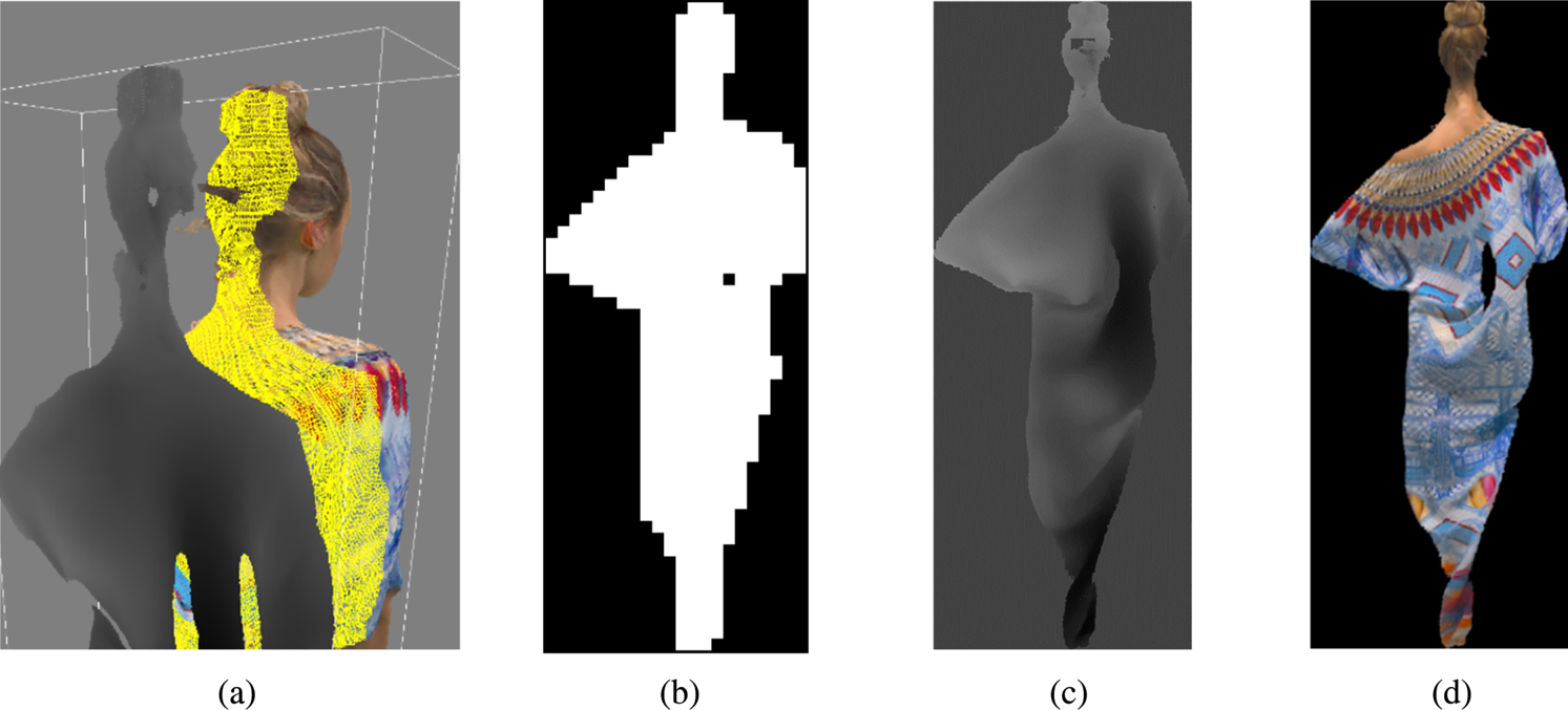
Fig. 3. 3D Patch projection and respective occupancy map, geometry, and attribute 2D images, (a) 3D patch, (b) 3D Patch Occupancy Map, (c) 3D Patch Geometry Image, (d) 3D Patch Texture Image.
B) V-PCC codec architecture
This section discusses some of the main functional elements/tools of V-PCC codec architecture, mainly: patch generation, packing, occupancy map, geometry, attribute(s), atlas image generation, image padding, and video compression. It should be noted that the functionalities provided by each of the listed tools can be implemented in different ways and methods. Specific implementation of these functionalities is non-normative and is not specified by the V-PCC standards. It thus becomes an encoder choice, allowing flexibility and differentiation.
During the standardization of V-PCC, a reference software (TMC2) has been developed, in order to measure the coding performance and to compare the technical merits/advantages of proposed point cloud coding methods that are being considered by V-PCC. The TMC2 encoder applies several techniques to improve coding performance, including how to perform packing of patches, the creation of occupancy maps, geometry, texture images, and the compression of occupancy map, geometry, texture, and patch information. Notice that TMC2 uses HEVC to encode the generated 2D videos but using HEVC is not mandatory and any appropriate image/video codec could also be used. Nevertheless, the architecture and results presented in this paper use HEVC as the base encoder. The TMC2 encoder architecture is illustrated in Fig. 4. The next sub-sections will provide details on each of the encoding blocks shown below.
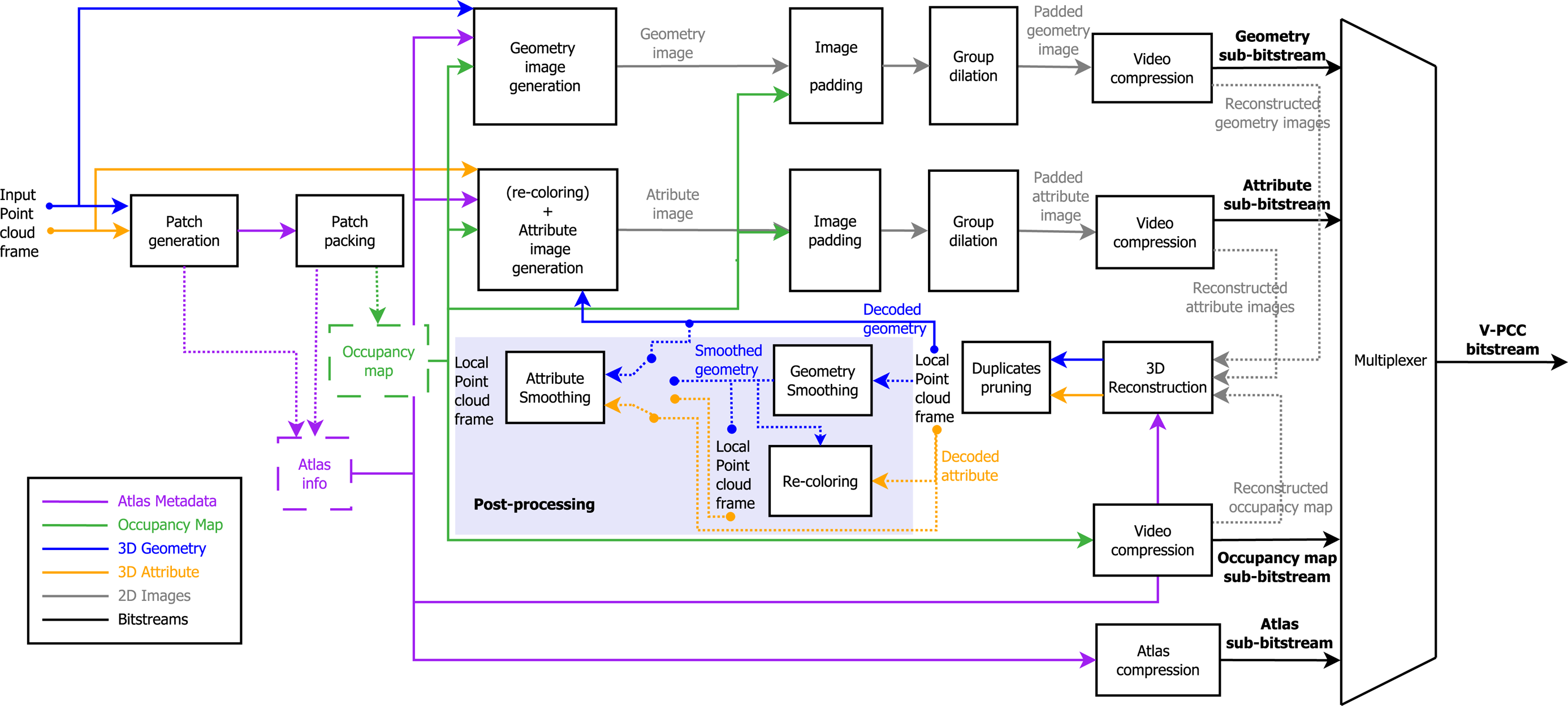
Fig. 4. TMC2 (V-PCC reference test model) encoder diagram [28].
1) Patch generation
Here we describe how to generate 3D patches in TMC2. First the normal for each point is estimated [Reference Hoppe, DeRose, Duchamp, McDonald and Stuetzle29]. Given the six orthographic projection directions (±x, ± y, ± z), each point is then associated with the projection direction that yields the largest dot product between the point's normal, and the corresponding projection direction is selected. The point classification is further refined according to the classification of neighboring points' projection direction. Once the points' classification is finalized, points with the same projection directions (category) are grouped together using a connected components algorithm. As a result of this process, each connected component is then referred to as a 3D patch. The 3D patch points are then projected orthogonally to one of the six faces of the axis-aligned bounding box based on their associated 3D patch projection direction. Notice that since the projection surface lies on a bounding box that is axis-aligned, two of the three coordinates of the point remains unchanged after projection, the third coordinate of the point is registered as a distance function between the point's location in 3D space and the projection surface (Fig. 5).
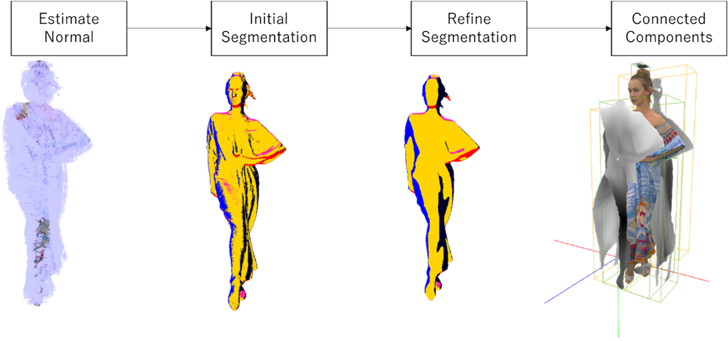
Fig. 5. Patch generation.
Since a 3D patch may have multiple points projected onto the same pixel location, TMC2 uses several “maps” to store these overlapped points. In particular, let us assume that we have a set of points H(u,v) being projected onto the same (u,v) location. Accordingly, TMC2 can, for example, decide to use two maps: a near map and a far map. The near map stores the point from H(u,v) with the lowest depth value D0. The far map stores the point with the highest depth value within a user-defined interval (D0, D0 + D). The user-defined interval size D represents the surface thickness and can be set by the encoder and used to improve geometry coding and reconstruction.
TMC2 has the option to code the far map as either a differential map from the near map in two separate video streams, or temporally interleave the near and far maps into one single stream and code the absolute values [Reference Guede, Cai, Ricard and Llach30]. In both cases, the interval size D can be used to improve the depth reconstruction process, since the reconstructed values must lie within the predefined interval (D0, D0 + D). The second map can be dropped altogether, and only an interpolation scheme is used to generate the far map [Reference Guede, Ricard and Llach31]. Furthermore, both frames can be sub-sampled and spatially interleaved in order to improve the reconstruction quality compared to reconstruction with one single map only, and coding efficiency compared to sending both maps [Reference Dawar, Najaf-Zadeh, Joshi and Budagavi32].
The far map can potentially carry the information of multiple elements mapped to the same location. In lossless mode, TMC2 modifies the far map image so that instead of coding a single point per sample, multiple points can be coded using an enhanced delta-depth (EDD) code [Reference Cai and Llach33]. The EDD code is generated by setting the EDD code bits to one to indicate whether a position is occupied between the near depth value D0 and the far depth value D1. This code is then added on top of the far map. In this way, multiple points can be represented by just using two maps.
It is however still possible to have some points that might be missing, and the usage of only six projection directions may limit the reconstruction quality of the point cloud. In order to improve the reconstruction of arbitrarily oriented surfaces, 12 new modes corresponding to cameras positioned at 45-degree direction were added to the standard [Reference Kuma and Nakagami34]. Notice that the rotation of point cloud to 45 degrees can be modeled using integer operations only, thus avoiding resampling issues caused by rotations.
To generate images suitable for video coding, TMC2 has added the option to perform filtering operations. For example, TMC2 defines a block size T × T (e.g. T = 16), within which depth values cannot have large variance, and points with depth values above a certain threshold are removed from the 3D patch. Furthermore, TMC2 defines a range to represent the depth, and if a depth value is larger than the allowed range, it is taken out of the 3D patch. Notice that the points removed from the 3D patch will be later analyzed by the connected components algorithm and may be used to generate a new 3D patch. Further improvements in 3D patch generation include using color information for plane segmentation [Reference Rhyu, Oh, Budagavi and Sinharoy35] and adaptively selecting the best plane for depth projection [Reference Rhyu, Oh, Budagavi and Sinharoy36].
TMC2 has the option to limit the minimum number of points in a 3D patch as a user-defined parameter. It therefore will not allow the generation of the 3D patch that may contain a lower number of points than the specified minimum number of points. Still, if these rejected points are within a certain user-defined threshold from the encoded point cloud, they may also not be included in any other regular patch. For lossy coding, TMC2 might decide to simply ignore such points. On the other hand, for lossless coding, points that are not included in any patch may be encoded by additional patches for lossless coding. These additional patches, known as auxiliary patches, store the (x, y, z) coordinates directly in the geometry image D0 created for regular patches, for 2D video coding. Alternatively, auxiliary patches can be stored in a separate image and coded as an enhancement image.
2) Patch packing
Patch packing refers to the placement of projected 2D patches in a 2D image of size W × H. This is an iterative process: first, the patches are ordered by their sizes. Then, the location of each patch is determined by an exhaustive search in raster scan order, and the first location that guarantees overlap-free insertion (i.e. all the T × T blocks occupied by the patch are not occupied by another patch in the atlas image) is selected. To improve fitting chances, eight different patch orientations (four rotations combined with or without mirroring) are also allowed [Reference Graziosi37]. Blocks that contain pixels with valid depth values (as indicated by the occupancy map) belonging to the area and covered by the patch size (rounded to a value that is a multiple of T) are considered as occupied blocks, and cannot be used by other patches, guaranteeing therefore that every T × T block is associated with only one unique patch. In the case that there is no empty space available for the next patch, the height H of the image is doubled, and the insertion of this patch is evaluated again. After insertion of all patches, the final height is trimmed to the minimum needed value. Figure 6 shows an example of packed patches' occupancy map, geometry, and texture images.
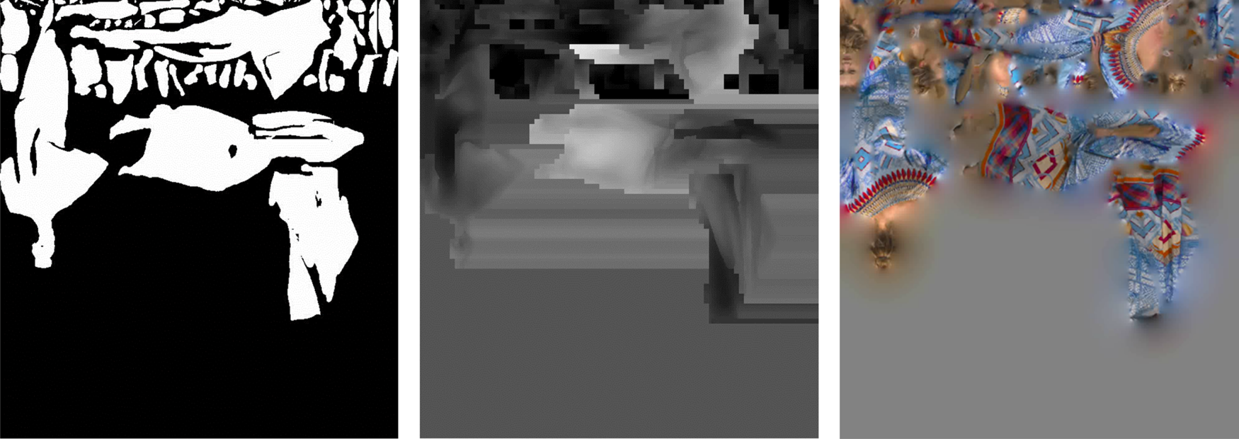
Fig. 6. Example of patch packing.
To improve compression efficiency, patches with similar content should be placed in similar positions across time. For the generation of a temporally consistent packing, TMC2 finds matches between patches of different frames and tries to insert matched patches at a similar location. For the patch matching operation, TMC2 uses the intersection over union (IOU) to find the amount of overlap between two projected patches [Reference Zhang38], according to the following equation:
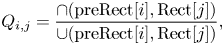
where preRect[i] is the 2D bounding box of the patch[i] from previous frame projected in 2D space. Rect[j] is the bounding box of the patch[j] from current frame projected in 2D space. $\cap ( {{\rm preRect}[ i ], {\rm Rect}[ j ] } )$ is the intersection area between preRect[i] and Rect[j] and $\cup ( {{\rm preRect}[ i ], {\rm Rect}[ j ] } ) \;$
 is the union area between preRect[i] and Rect[j].
The maximum IOU value determines a potential match between patch[i] and patch[j] from the previous frame. If the IOU value is larger than a pre-defined threshold, the two patches are considered to be matched, and information from the previous frame is used for packing and coding of the current patch. For example, TMC2 uses the same patch orientation and normal direction for matched patches, and only differentially encodes the patch position and bounding box information.
The patch matching information can be used to place the patches in a consistent manner across time. In [Reference Graziosi and Tabatabai39], space in the atlas is pre-allocated to avoid patch collision and guarantee temporal consistency. Further optimizations of the patch locations may consider different aspects besides only compression performance. For example, in [Reference Kim, Tourapis and Mammou40], the patch placement process was modified to allow low delay decoding, that is, the decoder does not need to wait to decode the information of all the patches to extract the block-to-patch information from the projected 2D images and can immediately identify which pixels belong to which patches as they are being decoded.
3) Geometry and occupancy maps
In contrast to geometry images defined in [Reference Gu, Gortler and Hoppe26, Reference Sander, Wood, Gortler, Snyder and Hoppe27], which store (x,y,z) values in three different channels, geometry images in V-PCC store the distance between the missing coordinates of points' 3D position and the projection surface in the 3D bounding box, using only the luminance channel of a video sequence. Since patches can have arbitrary shapes, some pixels may stay empty after patch packing. To differentiate between the pixels in the geometry video that are used for 3D reconstruction and the unused pixels, TMC2 transmits an occupancy map associated with each point cloud frame. The occupancy map has a user-defined precision of B × B blocks, where for lossless coding B = 1 and for lossy coding, usually B = 4 is used, with visually acceptable quality, while reducing significantly the number of bits required to encode the occupancy map.
The occupancy map is a binary image that is coded using a lossless video encoder [Reference Valentin, Mammou, Kim, Robinet, Tourapis and Su41]. The value 1 indicates that there is at least one valid pixel in the corresponding B × B block in the geometry video, while a value of 0 indicates an empty area that was filled with pixels from the image padding procedure. For video coding, a binary image of dimensions (W/B, H/B) is packed into the luminance channel and coded in lossless, but lossy coding of occupancy map is also possible [Reference Joshi, Dawar and Budagavi42]. Notice that for the lossy case, when the image resolution is reduced, the occupancy map image needs to be up scaled to a specified nominal resolution. The up-scaling process could lead to extra inaccuracies in the occupancy map, which has the end effect of adding points to the reconstructed point cloud.
4) Image padding, group dilation, re-coloring, and video compression
For geometry images, TMC2 fills the empty space between patches using a padding function that aims to generate a piecewise smooth image suited for higher efficiency video compression. Each block of T × T (e.g. 16 × 16) pixels is processed independently. If the block is empty (i.e. there are no valid depth values inside the block), the pixels of the block are filled by copying either the last row or column of the previous T × T block in raster scan order. If the block is full (i.e. all pixels have valid depth values), padding is not necessary. If the block has both valid and non-valid pixels, then the empty positions are iteratively filled with the average value of their non-empty neighbors. The padding procedure, also known as geometry dilation, is performed independently for each frame. However, the empty positions for both near and far maps are the same and using similar values can improve compression efficiency. Therefore, a group dilation is performed, where the padded values of the empty areas are averaged, and the same value is used for both frames [Reference Rhyu, Oh, Sinharoy, Joshi and Budagavi43].
A common raw format used as input for video encoding is YUV420, with 8-bit luminance and sub-sampled chroma channels. TMC2 packs the geometry image into the luminance channel only, since geometry represented by distance has only one component. Also, careful consideration of the encoding GOP structure can also lead to significant compression efficiency [Reference Zakharchenko and Solovyev44]. In the case of lossless coding, x-, y-, and z- coordinates of points that could not be represented in regular patches are block interleaved and are directly stored in the luminance channel. Moreover, 10-bit profiles such as the one in HEVC encoders [Reference Litwic45] can improve accuracy and coding performance. Additionally, hints for the placement of patches in the atlas can be given to the encoder to improve the motion estimation process [Reference Li, Li, Zakharchneko and Chen46].
Since the reconstructed geometry can be different from the original one, TMC2 transfers the color from the original point cloud to the decoded point cloud and uses these new color values for transmission. The recoloring procedure [Reference Kuma and Nakagami47] considers the color value of the nearest point from the original point cloud as well as a neighborhood of points closer to the reconstructed point to determine a possible better color value. Once the color values are known, TMC2 maps the color from 3D to 2D using the same mapping applied to geometry. To pad the color image, TMC2 may use a procedure based on mip-map interpolation and to further improve padding by using a sparse linear optimization model [Reference Graziosi48], as visualized in Fig. 7. The mip-map interpolation creates a multi-resolution representation of the texture image guided by the occupancy map, preserving active pixels even when they are down-sampled with empty pixels. A sparse linear optimization based on Gauss–Seidel relaxation can be used to fill in the empty pixels at each resolution scale. The lower resolutions are then used as initial values for the optimization of the up-sampled images at higher scale. In this way, the background is smoothly filled with values that are similar to the edges of the patches. Furthermore, the same principle of averaging positions that were before empty areas of maps (group dilation for geometry images) can be used for the attributes as well. The sequence of padded images is then color converted from RGB444 to YUV420 and coded with traditional video encoders.
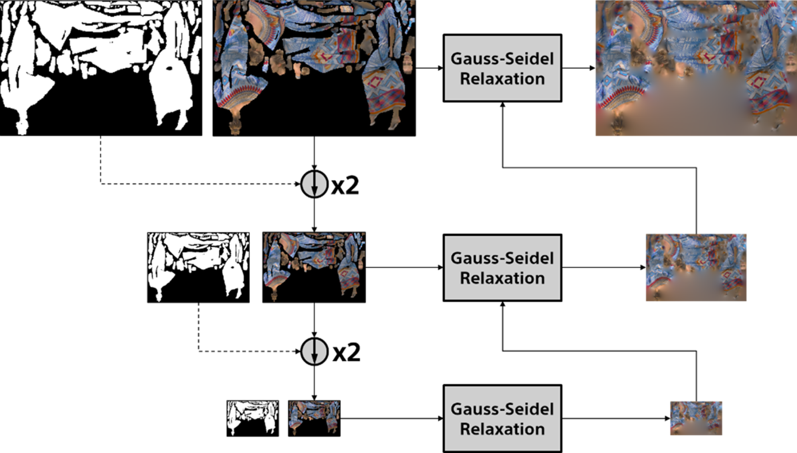
Fig. 7. Mip-map image texture padding with sparse linear optimization.
5) Duplicates pruning, geometry smoothing, and attribute smoothing
The reconstruction process uses the decoded bitstreams for occupancy map, geometry, and attribute images to reconstruct the 3D point cloud. When TMC2 uses two maps, the near and far maps, and the values from the two depth images are the same, TMC2 may generate several duplicate points. This can have an impact on quality, as well as the creation of unwanted points for lossless coding. To overcome this issue, the reconstruction process is modified to create only one point per (u,v) coordinate of the patch when the coordinates stored in the near map and the far map are equal [Reference Ricard, Guede, Llach, Olivier, Chevet and Gendron49], effectively pruning duplicate points.
The compression of geometry and attribute images and the additional points introduced due to occupancy map subsampling may introduce artifacts, which could affect the reconstructed point cloud. TMC2 can use techniques to improve the local reconstruction quality. Notice that similar post-processing methods can be signaled and done at the decoder side. For instance, to reduce possible geometry artifacts caused by segmentation, TMC2 may smooth the points at the boundary of patches using a process known as 3D geometry smoothing [Reference Nakagami50]. One potential candidate method for point cloud smoothing identifies the points at patch edges and calculates the centroid of the decoded points in a small 3D grid. After the centroid and the number of points in the 2 × 2 × 2 grid is derived, a commonly used trilinear filter is applied.
Due to the point cloud segmentation process and the patch allocation, which may place patches with different attributes near each other in the images, color values at patch boundaries may be prone to visual artifacts as well. Furthermore, coding blocking artifacts may create reconstruction patterns that are not smooth across patch boundaries, creating visible seams artifacts in the reconstructed point cloud. TMC2 has the option to perform attribute smoothing [Reference Joshi, Najaf-Zadeh and Budagavi51] to reduce the seams effect on the reconstructed point cloud. Additionally, the attribute smoothing is performed in 3D space, to utilize the correct neighborhood when estimating the new smoothed value.
6) Atlas compression
Many of the techniques explained before have non-normative aspects, meaning that they are performed at the encoder only, and the decoder does not need to be aware of them. However, a couple of aspects, especially related to the metadata that is used to reconstruct the 3D data from the 2D video data, is normative and need to be sent to the decoder for proper processing. For example, the position and the orientation of patches, the block size used in the packing, and others are all atlas metadata that need to be transmitted to the decoder.
The V-PCC standard defines an atlas metadata stream based on NAL units, where the patch data information is transmitted. The NAL unit structure is similar to the bitstream structure used in HEVC [Reference Sullivan, Ohm, Han and Wiegand3], which allows for greater encoding flexibility. Description of normative syntax elements as well as the explanation of coding techniques for the metadata stream, such as inter prediction of patch data, can be found in the current standard specification [52].
IV. GEOMETRY-BASED POINT CLOUD CODING
In the following sub-sections, we describe the coding principle of G-PCC and explain some of its coding tools.
A) Geometry-based coding principle
While the V-PCC coding approach is based on 3D to 2D projections, G-PCC, on the contrary, encodes the content directly in 3D space. In order to achieve that, G-PCC utilizes data structures, such as an octree that describes the point locations in 3D space, which is explained with further detail in the next section. Furthermore, G-PCC makes no assumption about the input point cloud coordinate representation. The points have an internal integer-based value, converted from a floating point value representation. This conversion is conceptually similar to voxelization of the input point cloud, and can be achieved by scaling, translation, and rounding.
Another key concept for G-PCC is the definition of tiles and slices to allow parallel coding functionality [Reference Shao, Jin, Li and Liu53]. In G-PCC, a slice is defined as a set of points (geometry and attributes) that can be independently encoded and decoded. In its turn, a tile is a group of slices with bounding box information. A tile may overlap with another tile and the decoder can decode a partial area of the point cloud by accessing specific slices.
One limitation of the current G-PCC standard is that it is only defined for intra prediction, that is, it does not currently use any temporal prediction tool. Nevertheless, techniques based on point cloud motion estimation and inter prediction are being considered for the next version of the standard.
B) G-PCC codec architecture: TMC13
Figure 8 shows a block diagram depicting the G-PCC reference encoder [54], also known as TMC13, which will be described in the next sections. It is not meant to represent TMC13's complete set of functionalities, but only some of its core modules. First, one can see that geometry and attributes are encoded separately. However, attribute coding depends on decoded geometry. As a consequence, point cloud positions are coded first.
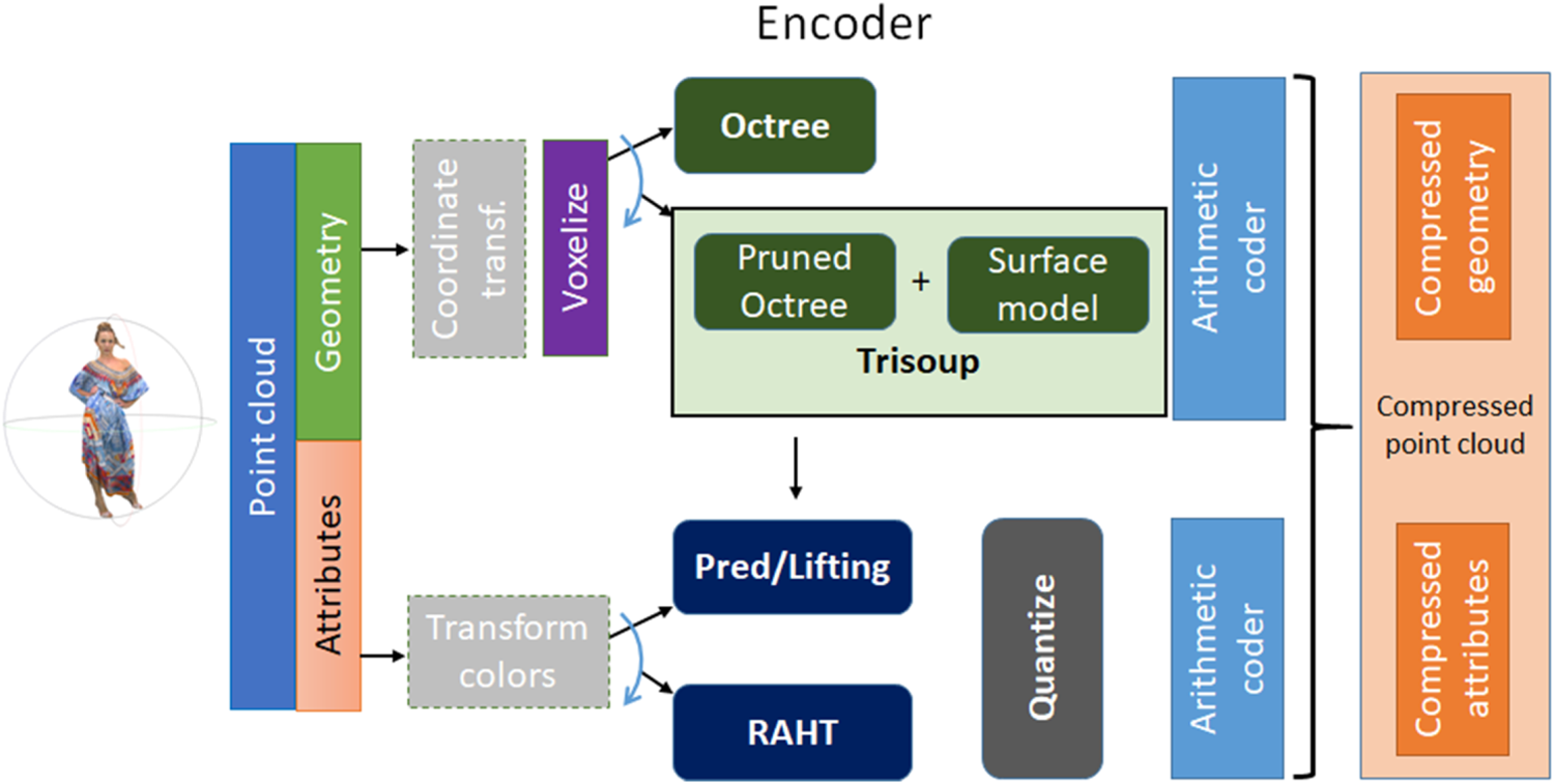
Fig. 8. G-PCC reference encoder diagram.
Source geometry points may be represented by floating point numbers in a world coordinate system. Thus, the first step of geometry coding is to perform a coordinate transformation followed by voxelization. The second step consists of the geometry analysis using the octree or trisoup scheme, as discussed in Sections IV.B.1 and IV.B.2 below. Finally, the resulting structure is arithmetically encoded. Regarding attributes coding, TMC13 supports an optional conversion from RGB to YCbCr [55]. After that, one of the three available transforming tools is used, namely, the Region Adaptive Hierarchical Transform (RAHT), the Predicting Transform, and the Lifting Transform. These transforms are discussed in Section IV.B.3. Following the transform, the coefficients are quantized and arithmetically encoded.
1) Octree coding
The voxelized point cloud is represented using an octree structure [Reference Meagher56] in a lossless manner. Let us assume that the point cloud is contained in a quantized volume of D × D × D voxels. Initially, the volume is segmented vertically and horizontally into eight sub-cubes with dimensions D/2 × D/2 × D/2 voxels, as exemplified in Fig. 9. This process is recursively repeated for each occupied sub-cube until D is equal to 1. It is noteworthy to point out that in general only 1% of voxel positions are occupied [Reference de Queiroz and Chou57], which makes octrees very convenient to represent the geometry of a point cloud. In each decomposition step, it is verified which blocks are occupied and which are not. Occupied blocks are marked as 1 and unoccupied blocks are marked as 0. The octets generated during this process represent an octree node occupancy state in 1-byte word and are compressed by an entropy coder considering the correlation with neighboring octets. For the coding of isolated points, since there are no other points within the volume to correlate with, an alternative method to entropy coding the octets, namely Direct Coding Mode (DCM), is introduced [Reference Lassere and Flynn58]. In DCM, coordinates of the point are directly coded without performing any compression. DCM mode is inferred from neighboring nodes in order to avoid signaling the usage of DCM for all nodes of the tree.
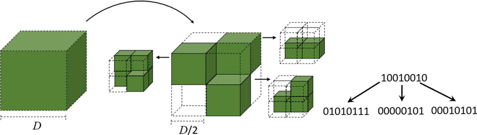
Fig. 9. First two steps of an octree construction process.
2) Surface approximation via trisoup
Alternatively, the geometry may be represented by a pruned octree, constructed from the root to an arbitrary level where the leaves represent occupied sub-blocks that are larger than a voxel. The object surface is approximated by a series of triangles, and since there is no connectivity information that relates the multiple triangles, the technique is called “triangle soup” (or trisoup). It is an optional coding tool that improves the subjective quality in lower bitrate as the quantization gives the rough rate adaptation. If trisoup is enabled, the geometry bitstream becomes a combination of octree, segment indicator, and vertex position information. In the decoding process, the decoder calculates the intersection point between the trisoup mesh plane and the voxelized grid as shown in [Reference Nakagami59]. The number of the derived points in the decoder is determined by the voxel grid distance d, which can be controlled [Reference Nakagami59] (Fig. 10).
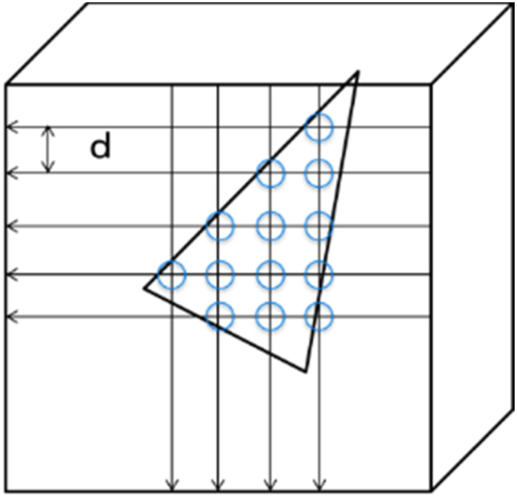
Fig. 10. Trisoup point derivation at the decoder.
3) Attribute encoding
In G-PCC, there are three methods for attribute coding, which are: (a) RAHT [Reference de Queiroz and Chou57]; (b) Predicting Transform [60]; and (c) Lifting Transform [Reference Mammou, Tourapis, Kim, Robinet, Valentin and Su61]. The main idea behind RAHT is to use the attribute values in a lower octree level to predict the values in the next level. The Predicting Transform implements an interpolation-based hierarchical nearest-neighbor prediction scheme. The Lifting Transform is built on top of Predicting Transform but has an extra update/lifting step. Because of that, from this point forward they will be jointly referred to as Predicting/Lifting Transform. The user is free to choose either of the above-mentioned transforms. However, given a specific context, one method may be more appropriate than the other. The common criterion that determines which method to use is a combination of rate-distortion performance and computational complexity. In the next two sections, RAHT and Predicting/Lifting attribute coding methods will be described.
RAHT Transform. The RAHT is performed by considering the octree representation of the point cloud. In its canonical formulation [Reference de Queiroz and Chou57], it starts from the leaves of the octree (highest level) and proceeds backwards until it reaches its root (lowest level). The transform is applied to each node and is performed in three steps, one in each x, y, and z directions, as illustrated in Fig. 11. At each step, the low-pass g n and high-pass h n coefficients are generated.
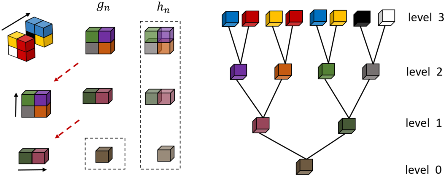
Fig. 11. Transform process of a 2 × 2 × 2 block.
RAHT is a Haar-inspired hierarchical transform. Thus, it can be better understood if a 1D Haar transform is taken as an initial example. Consider a signal v with N elements. The Haar decomposition of v generates g and h, which are the low-pass and high-pass components of the original signal, each one with N/2 elements. The n-th coefficients of g and h are calculated using the following equation:
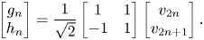
The transform can be performed recursively taking the current g as the new input signal v, and at each recursion the number of low-pass coefficients is divided by a factor of 2. The g component can be interpreted as a scaled sum of equal-weighted consecutive pairs of v, and the h component as their scaled difference. However, if one chooses to use the Haar transform to encode point clouds, the transform must be modified to take the sparsity of the input point cloud into account. This can be accomplished by allowing the weights to adapt according to the distribution of points. Hence, the recursive implementation of the RAHT can be defined as follows:
where l is the decomposition level, w 1 and w 2 are the weights associated with the $g_{2n}^{l + 1}$ and $g_{2n + 1}^{l + 1}$
 low-pass coefficients at level l + 1, and $w_n^l$
 is the weight of the low-pass coefficient $g_n^l$
 at level l. As a result, higher weights are applied to the dense area points so that the RAHT can balance the signals in the transform domain better than the non-adaptive transform.
A fixed-point formulation of RAHT was proposed in [Reference Sandri, Chou, Krivokuća and de Queiroz62]. It is based on matrix decompositions and scaling of quantization steps. Simulations showed that the fixed-point implementation can be considered equivalent to its floating-point counterpart.
Most recently, a transform domain prediction in RAHT has been proposed [Reference Flynn and Lasserre63] and is available in the current test model TMC13. The main idea is that for each block, the transformed upconverted sum of attributes at level d, calculated from the decoded sum of attributes at d–1, is used as a prediction to the transformed sum of attributes at level d, generating high-pass residuals that can be further quantized and entropically encoded. The upconverting process is accomplished by means of a weighted average of neighboring nodes. Figure 12 shows a simplified illustration of the previously described prediction scheme. Reported gains over RAHT formulation without prediction show significant improvements in a rate-distortion sense (up to around 30% overall average gains for color and 16% for reflectance).
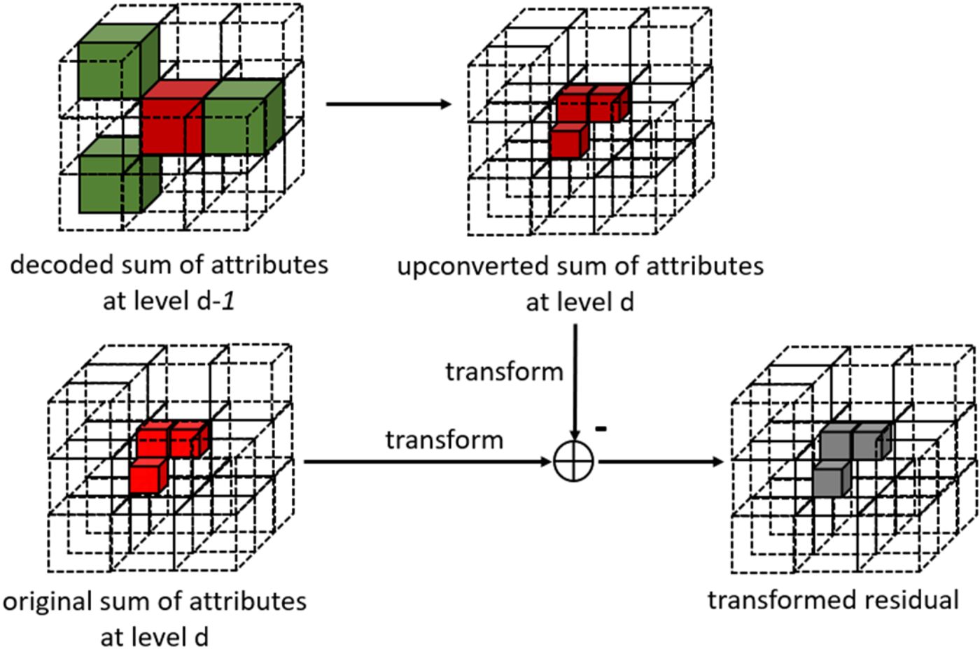
Fig. 12. Example of upconverted transform domain prediction in RAHT.
Predicting/Lifting Transform. The Predicting Transform is a distance-based prediction scheme for attribute coding [60]. It relies on a Level of Detail (LoD) representation that distributes the input points in sets of refinements levels (R) using a deterministic Euclidean distance criterion. Figure 13 shows an example of a sample point cloud organized in its original order, and reorganized into three refinement levels, as well as the correspondent Levels of Details (LoD0, LoD1, and LoD2). One may notice that a level of detail l is obtained by taking the union of refinement levels for 0 to l.
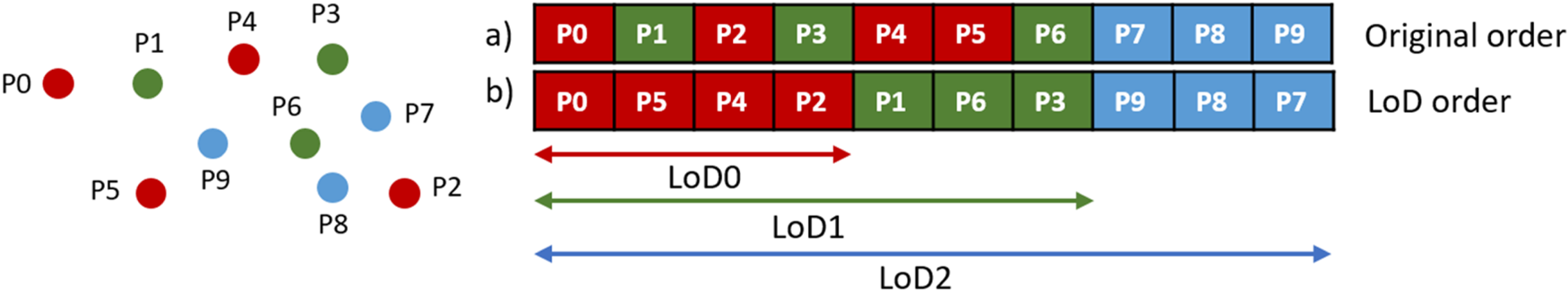
Fig. 13. Levels of detail generation process.
The attributes of each point are encoded using a prediction determined by the LoD order. Using Fig. 13 as an illustration, consider LoD0 only. In this specific case, the attributes of P2 can be predicted by the reconstructed versions of its nearest neighbors, P4, P5, or P0, or by a distance-based weighted average of these points. The maximum number of prediction candidates can be specified, and the number of nearest neighbors is determined by the encoder for each point. In addition, a neighborhood variability analysis [60] is performed. If the maximum difference between any two attributes in the neighborhood of a given point P is higher than a threshold, a rate-distortion optimization procedure is used to control the best predictor. By default, the attribute values of a refinement level R(j) are always predicted using the attribute values of its k-nearest neighbors in the previous LoD, that is, LoD(j–1). However, prediction within the same refinement level can be performed by setting a flag to 1 [64], as shown in Fig. 14.
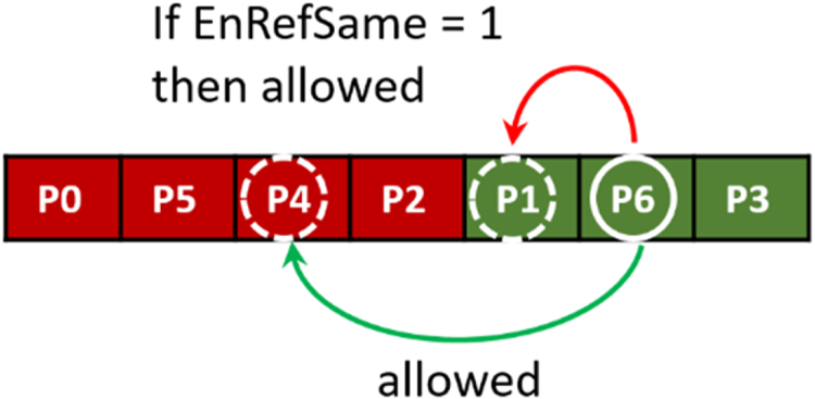
Fig. 14. LoD referencing scheme.
The Predicting Transform is implemented using two operators based on the LoD structure, which are the split and merge operators. Let L(j) and H(j) be the sets of attributes associated with LoD(j) and R(j), respectively. The split operator takes L(j + 1) as an input and returns the low-resolution samples L(j) and the high-resolution samples H(j). The merge operator takes L(j) and H(j) and returns L(j + 1). The predicting scheme is illustrated in Fig. 15. Initially, the attributes signal L(N + 1), which represents the whole point cloud, is split into H(N) and L(N). Then L(N) is used to predict H(N) and the residual D(N) is calculated. After that, the process goes on recursively. The reconstructed attributes are obtained through the cascade of merge operations.
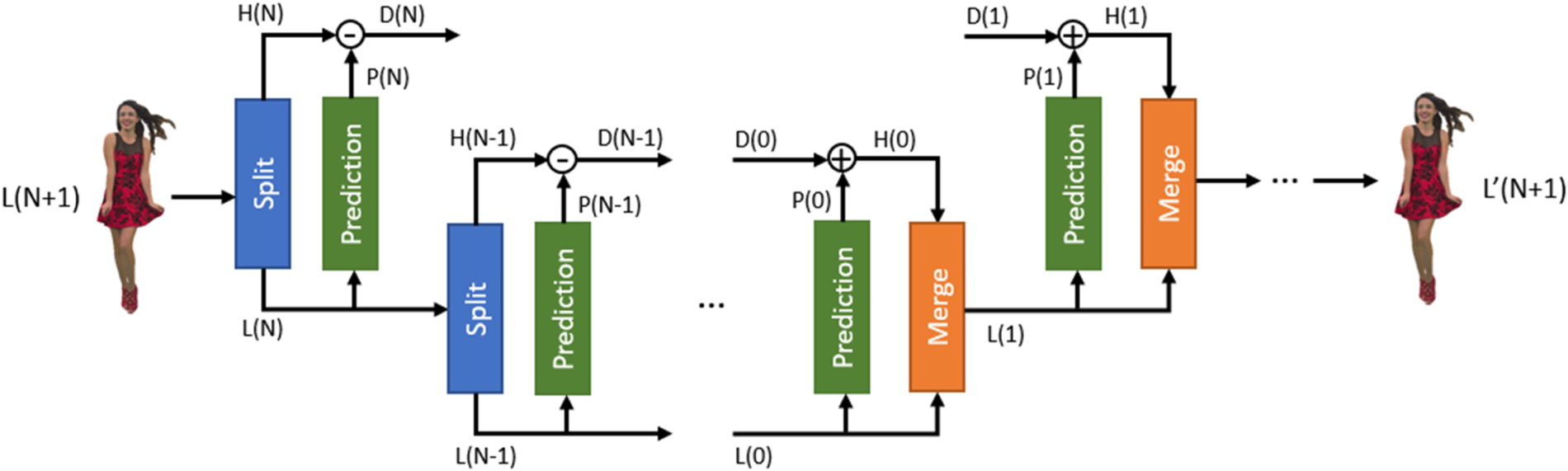
Fig. 15. Forward and Inverse Predicting Transform.
The Lifting Transform [Reference Mammou, Tourapis, Kim, Robinet, Valentin and Su61], represented in the diagram of Fig. 16, is built on top of the Predicting Transform. It introduces an update operator and an adaptive quantization strategy. In the LoD prediction scheme, each point is associated with an influence weight. Points in lower LoDs are used more often and, therefore, impact the encoding process more significantly. The update operator determines U(j) based on the residual D(j) and then updates the value of L(j) using U(j), as shown in Fig. 16. The update signal U(j) is a function of the residual D(j), the distances between the predicted point and its neighbors, and their correspondent weights. Finally, to guide the quantization processes, the transformed coefficients associated with each point are multiplied by the square root of their respective weights.
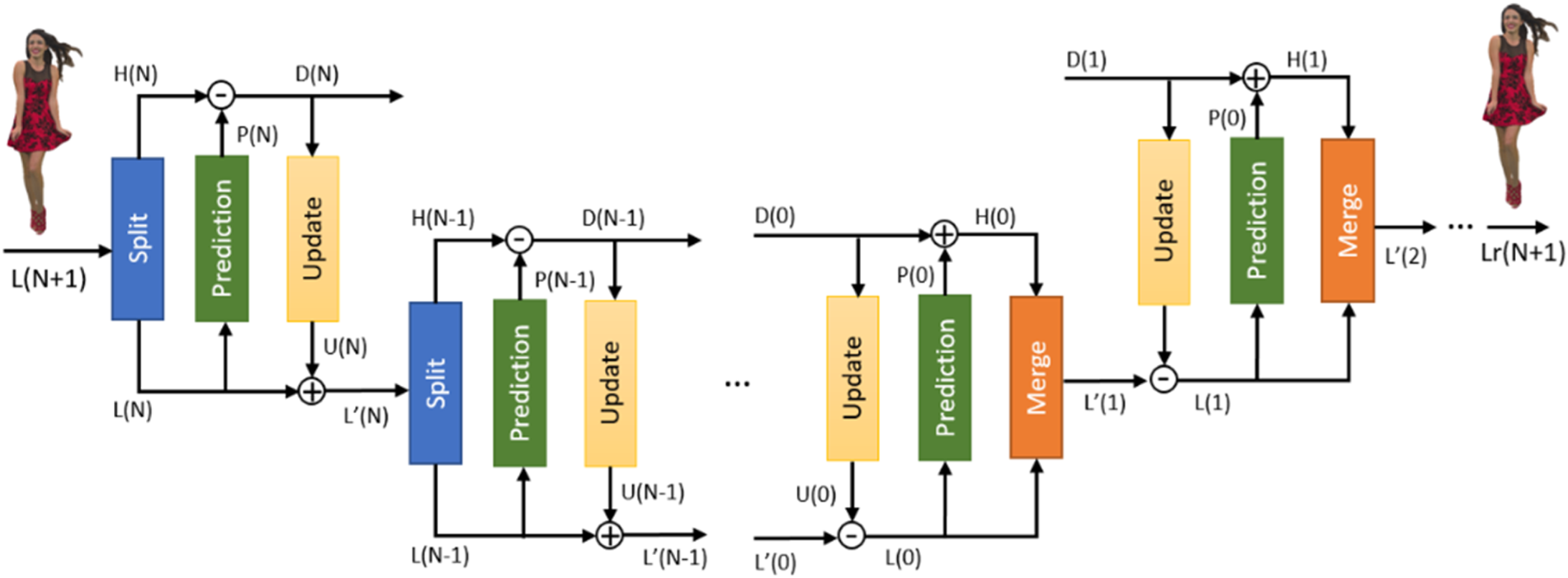
Fig. 16. Forward and Inverse Predicting/Lifting Transform.
V. POINT CLOUD COMPRESSION PERFORMANCE
In this section, we will show the performance of V-PCC for AR/VR use case, that is, coding dynamic point cloud sequences, and G-PCC for heritage collection and autonomous driving. Geometry and attributes are encoded using the latest reference software (TMC2v8.0 [25] and TMC13v7.0 [54]) following the common test conditions (CTC, [65]) set by the MPEG group. Furthermore, distortions due to compression artifacts are measured with the pc_error tool [Reference Tian, Ochimizu, Feng, Cohen and Vetro66], where in addition to geometric distortion from point-to-point (D1) and point-to-plane (D2), attribute distortion in terms of PSNR and bitrates are also reported. The part of the PCC dataset that is used in our simulations is depicted in Fig. 17. The results presented here can be reproduced by following the CTC [65].
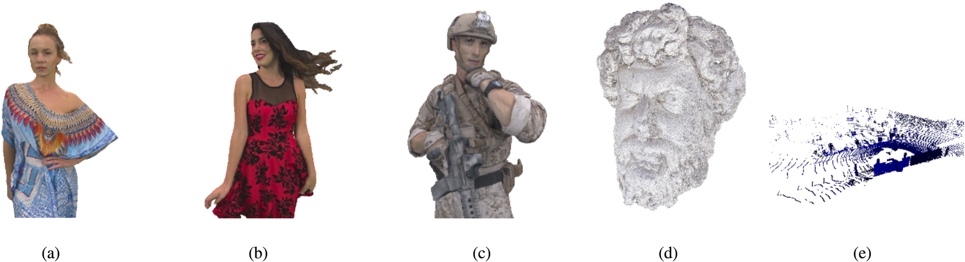
Fig. 17. Point cloud test set, (a) Longdress, (b) Red and Black, (c) Soldier, (d) Head, (e) Ford.
A) V-PCC performance
Here we show the compression performance of TMC2 to encode dynamic point cloud sequences, such as Longdress, Red and Black, and Soldier sequences [Reference Tudor1]. These are composed of a 10 s point cloud sequence of a human subject at 30 frames per second. Each point cloud frame has approximately 1 million points, with voxelized positions and RGB color attributes. Since the beginning of the standardization process, the reference software performance has improved significantly, as shown in the graphs depicted by Fig. 18. For example, for the longdress sequence, the gain achieved with TMC2v8.0 compared against TMC2v1.0 is about 60% savings in BD-rate for the point-to-point metric (D1) and about 40% savings in BD-rate for the luma attribute.
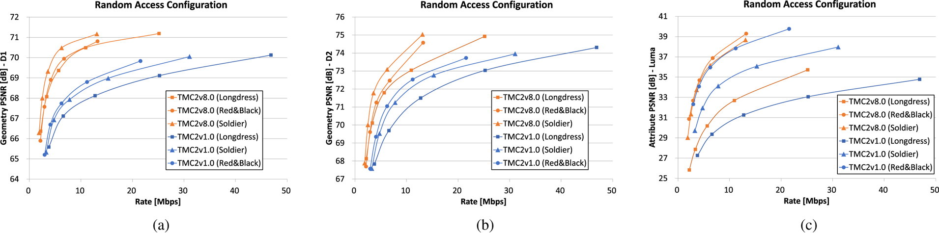
Fig. 18. TMC2v1.0 versus TMC2v8.0, (a) Point-to-point geometry distortion (D1), (b) Point-to-plane geometry distortion (D2) (c), Luma attribute distortion.
Both point-to-point and point-to-plane metrics show the efficiency of the adopted techniques. Furthermore, improvement in the RD performance for attributes can also be verified. As TMC2 relies on the existing video codec for the compression performance, the improvement mostly comes from the encoder optimization such as a patch allocation among frames in time consistency manner [Reference Graziosi and Tabatabai39], or motion estimation guidance for the video coder from the patch generator [Reference Li, Li, Zakharchneko and Chen46].
Figure 19 provides a visualization of the coded sequences using MPEG PCC Reference Rendering Software [67]. With the latest TMC2 version 8, the 10–15 Mbps bitstream provides a good visual quality over the 70 dB while the initial TM v1 needed 30–40 Mbps for the same quality.
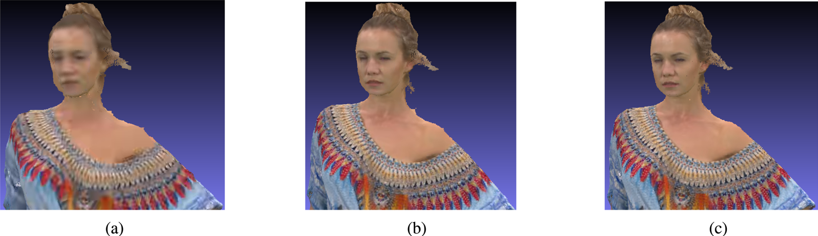
Fig. 19. Subjective quality using PCC Rendering Software, (a) Longdress at 2.2 Mbps, (b) Longdress at 10.9 Mbps, (c) Longdress at 25.2 Mbps.
B) G-PCC performance
There are different encoding scenarios involving geometry representation (octree or trisoup), attributes transform (RAHT, Predicting, or Lifting Transforms), as well as compression methods (lossy, lossless, and near-lossless). Depending on the use case, a subset of these tools is selected. In this section, we show a comparison between RAHT and Predicting/Lifting Transforms, both using lossless octree geometry and lossy attribute compression schemes. Results for two point clouds that represent specific use cases are presented. The first point cloud (head_00039_vox12, about 14 million points) is an example of cultural heritage application. In this use case, point clouds are dense, and color attribute preservation is desired. The second point cloud (ford_01_q1 mm, about 80 thousand points per frame) is in fact a sequence of point clouds, and represents the autonomous driving application. In this use case, point clouds are very sparse, and in general reflectance information preservation is desired. Figure 20(a) shows luminance PSNR plots (Y-PSNR) for head_00039_vox12 encoded with RAHT (with and without transform domain prediction) and Lifting Transform. Figure 20(b) shows reflectance PSNR plots (R-PSNR) for ford_01_q1 mm encoded with the same attribute encoders. As stated before, in both cases, geometry is losslessly encoded.
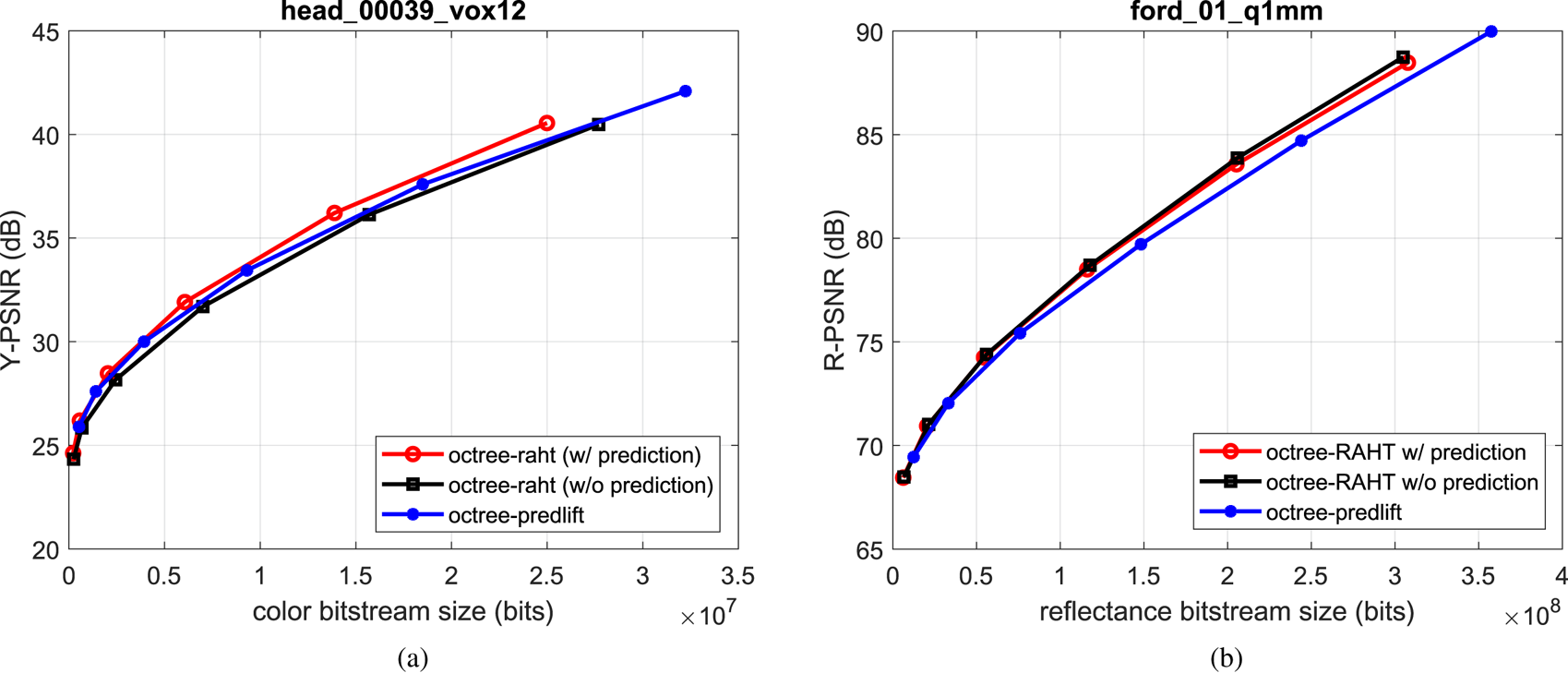
Fig. 20. Examples of G-PCC coding performance.
PSNR plots show that for head_00039_vox12, RAHT with transform domain prediction outperforms RAHT without prediction and the Lifting Transform in terms of luminance rate-distortion. For ford_01_q1 mm, RAHT outperforms Lifting; however, turning off the transform domain prediction yields slightly better results.
As for lossless geometry and lossless attribute compression, Predicting Transform is used. In this case, considering both geometry and attributes, the compression ratios for head_00039_vox12 and ford_01_q1 mm are around 3 to 1 and 2 to 1, respectively. Taking all the point clouds in the CTC into account, the average compression ratio is around 3 to 1. A comparison with the open-source 3D codec Draco [68] was performed in [Reference Flynn and Lasserre69]. For the same point clouds, the observed compression ratios for Draco were around 1.7 in both cases. Again, considering all the CTC's point clouds, the average compression ratio for Draco is around 1.6 to 1. In summary, current TMC13 implementation has outperformed Draco by a factor of 2 to 1 for lossless compression.
VI. CONCLUSION
Recent progress in 3D capture technologies has provided tremendous opportunities for capture and generation of 3D visual data. A unique aspect of PCC standardization work has been the joint participation of both video coding and computer graphics experts, working together to provide a 3D codec standard incorporating state-of-the-art technologies from both 2D video coding and computer graphics.
In this paper, we presented the main concepts related to PCC, such as point cloud voxelization, 3D to 2D projection, and 3D data structures. Furthermore, we provided an overview of the coding tools used in the current test models for V-PCC and G-PCC standards. For V-PCC, topics such as patch generation, packing, geometry, occupancy map, attribute image generation, and padding were discussed. For G-PCC, topics such as octree, trisoup geometry coding, and 3D attribute transforms such as RAHT and Predicting/Lifting were discussed. Some illustrative results of the compression performance of both encoding architectures were presented and results indicate that these tools achieve the current state-of-the-art performance in PCC, considering use cases like dynamic point cloud sequences, world heritage collection, and autonomous driving.
It is expected that the two PCC standards provide competitive solutions to a new market, satisfying various application requirements or use cases. In the future, MPEG is also considering extending the PCC standards to new use cases, such as dynamic mesh compression for V-PCC, and including new tools, such as inter coding for G-PCC. For the interested reader, the MPEG PCC website [70] provides further informative resources as well as the latest test model software for V-PCC and G-PCC.
Danillo B. Graziosi received the B.Sc., M.Sc., and D.Sc. degrees in electrical engineering from the Federal University of Rio de Janeiro, Rio de Janeiro, Brazil, in 2003, 2006, and 2011, respectively. He is currently the Manager of the Next-Generation Codec Group at Sony's R&D Center US San Jose Laboratory. His research interests include video/image processing, light fields, and point cloud compression.
Ohji Nakagami received the B.Eng. and M.S. degrees in electronics and communication engineering from Waseda University, Tokyo, Japan, in 2002 and 2004, respectively. He has been with Sony Corporation, Tokyo, Japan, since 2004. Since 2011, he has been with the ITU-T Video Coding Experts Group and the ISO/IEC Moving Pictures Experts Group, where he has been contributing to video coding standardization. He is an Editor of the ISO/IEC committee draft for video-based point cloud compression (ISO/IEC 23090-5) and the ISO/IEC working draft for geometry-based point cloud compression (ISO/IEC 23090-9).
Satoru Kuma received the B.Eng. and M.Eng. degrees in information and system information engineering from Hokkaido University, Japan, in 1998 and 2000, respectively. He works at Sony Corporation, Tokyo, Japan. His research interests include video/image processing, video compression and point cloud compression.
Alexandre Zaghetto received his B.Sc. degree in electronic engineering from the Federal University of Rio de Janeiro (2002), his M.Sc. degree in 2004, and his Dr. degree in 2009 from the University of Brasilia (UnB), both in electrical engineering. Previous to his current occupation, he was an Associate Professor at the Department of Computer Science/UnB. Presently, Dr. Zaghetto works at Sony's R&D Center San Jose Laboratory, California, as a Senior Applied Research Engineer. He is a Senior Member of IEEE and his research interests include, but are not limited to, digital image and video processing, and point cloud compression.
Teruhiko Suzuki received the B.Sc. and M.Sc. degrees in physics from Tokyo Institute of Technology, Japan, in 1990 and 1992, respectively. He joined Sony Corporation in 1992. He worked for research and development for video compression, image processing, signal processing, and multimedia systems. He also participated in the standardization in ISO/IEC JTC1/SC29/WG11 (MPEG), ISO/IEC JTC1, ITU-T, JVT, JCT-VC, JVET, SMPTE, and IEC TC100.
Ali Tabatabai (LF'17) received the bachelor's degree in electrical engineering from Tohoku University, Sendai, Japan, and the Ph.D. degree in electrical engineering from Purdue University. He was the Vice President of the Sony US Research Center, where he was responsible for research activities related to camera signal processing, VR/AR capture, and next-generation video compression. He is currently a Consultant and a Technical Advisor to the Sony US Research Center and the Sony Tokyo R&D Center. He is an Editor of the ISO/IEC committee draft for video-based point cloud compression (ISO/IEC 23090-5).


 Open access