

I. INTRODUCTION
We are on the cusp of the rapid transformation from automation to intelligence in manufacturing, with the help of the industrial Internet-of-Things to create digital twins of the factories and manage digital data flow, and the use of Artificial Intelligence (AI) technology to reason the data. Recent surveys amongst companies in the field indicate an overwhelming belief that AI-related technologies will make a practical and visible impact, with manufacturing projected to be leading other industries in terms of AI market size [1]. While the volume of data created annually in manufacturing is leading other industries such as government, media, banking, retail, and healthcare, the data can be fragmented and difficult to acquire for external parties to process and analyze, owing to the nature of the industry. That is one of the reasons why it remains a challenging, lengthy, and mysterious process for external parties or technology providers when it comes to enabling AI within manufacturing facilities. In this article, we focus on several case studies related to our efforts in enabling AI and computer vision technology in a tier-one electronics maker, Inventec Inc. In this process, we hope to bring some light to the intricacies related to acquiring relevant data, defining valuable problems, and enabling smart manufacturing projects.
Inventec Inc. [2], founded in 1975 with headquarter located in Taipei, Taiwan, is a tier 1 original design electronics manufacturer, with annual revenue exceeding USD$16 billion in 2019. In addition to the facilities in Taiwan, Inventec operates production campuses around the world, including Shanghai, Nanjing, Chongqing (China), Brno (Czech Republic), and Juarez (Mexico), with regional office presence in Bay Area (California), Austin (Texas), and Tokyo (Japan). The company develops various kinds of products with its customers, ranging from personal computers, laptops, data center servers, mobile phones, smart devices, and medical devices. In Taiwan, it leads all other companies and research universities in terms of the number of global AI-related patents and intellectual properties as of 2018, as surveyed by the government-funded Industrial Technology Research Institute (ITRI) [3].
On average, Inventec produces over 20 million laptops, 4 million servers, and 75 million smart devices annually. Naturally, at this scale, it is imperative to have a sufficient level of automation to ensure quality consistency and cost efficiency to lower labor-related risks, including cost, availability, and, more recently, public health due to the COVID-19 global pandemic. The company has been very successful in this regard, by continuously optimizing the workflow and build process of the products. For example, the direct labor cost required to assemble a laptop has been reduced by more than half between 2017 and 2019 through careful optimization of the production line. However, parts of the production process still require human judgment during planning and manufacturing, and this remains the highest production risk according to internal surveys amongst our production engineers and managers. Because identifying and solving these problems are beyond the means of traditional manufacturing automation vendors, it becomes our mission at the Inventec AI Center is to discover, define, and develop solutions to these problems. In the remainder of the article, we shall discuss several critical problems that we helped solve in a laptop manufacturing facility, including
• A logistic management process for forecasting parts needed for manufacturing the products,
• A system for automatically qualifying products for mass production, and
• A methodology for creating visual inspection AI models with a small amount of defect data.
Before we dive into details for each project, we shall begin with some additional backgrounds on how to identify, enable projects with proofs-of-concept (POCs), and acquiring the necessary resources to bring them to production.
II. ENABLING SMART MANUFACTURING PROJECTS
An adequately managed manufacturing facility is cost-conscious, which means that, in many cases, an outside process innovation team may have difficulty accessing the facilities for experiments if these experiments cause potential production disruptions. Even as an inside team with blessings from the management, it remains crucial to ensure that any potential process improvements minimize the impact on the production lines while generating sufficient and measurable impact.
To maximize impact and to ensure we are working on the right problem, it would be necessary to view the manufacturing process holistically and define high-level goals before diving into individual projects. A successful smart manufacturing project would require a clear problem definition, with clean and unambiguous data blessed by the domain experts. Once a project becomes technically feasible, it can only enter production when it meets key return-on-investment (ROI) requirements. We discuss these issues in more detail in the following sections.
A) Problem Definition
A problem is defined correctly when multiple parties, including the factory floor managers, information technology officers, algorithm developers, mechanical engineers, and managers, come to terms with the goals and impact of the project. Bringing all parties to an agreement can be difficult, as the scope can be ambiguous, and the expectations toward AI technology can often be overly broad. Furthermore, the ownership of the project can be tricky to define, as it implies budgeting and personnel commitment, both of which can be difficult for cost-conscious manufacturing facilities to commit to before demonstrating clear benefits to the process.
As a result, we find that production-ready projects tend to be the ones with early commitments from the facilities, with tangible benefits (e.g. man-year saved) and precise requirements (e.g. process automation). These projects often come from middle-level management who have definite problems to solve but lack the technology or initial budget blessing to get the projects started. Furthermore, the case studies in this article focus on the projects that are difficult to implement using traditional, non-NN approaches, and therefore a direct comparison with traditional methods would not be feasible. Part of the reason is that existing automation and processes may have residual accounting values and tend to become lower priority items in the upgrade queue, unless if the new AI-based solution can significantly disrupt the existing solution.
Once we identify the problems with written specifications, it is also essential to form a cross-department task force to ensure that individual department KPIs do not conflict with the project goals. Most facilities have clearly defined goals (e.g. the pace of production, utility rate, labor usage), and almost any process improvement would cause temporary disruptions to these goals. Therefore, it is vital to include project goals into facility KPIs so that each party can communicate short-term negative impacts to the upper management.
B) Data in Manufacturing
Many modern AI algorithms require usable data for training purposes. Many companies nowadays have centralized Enterprise Resource Planning (ERP) systems. Therefore, financially related data are often not difficult to acquire from the ERP, and the size of the data is manageable for remote transport purposes. Two other types of data are, however, often siloed and challenging to acquire. These include machine state data from the factory floor and image data from individual inspection sites. Figure 1 refers to a high-level process where we enable the acquisition of these additional data through projects.
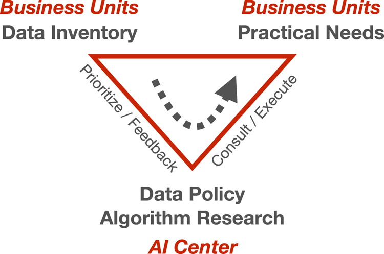
Fig. 1. Our roles within the company. Manufacturing data tend to scatter throughout various IT systems, and part of our mission is to normalize the data by enabling AI projects with apparent impacts for the business units. The arrow indicates data flow.
Machine state data, if available, would be stored in a Production Management System (PMS), and a virtual network often needs to be set up for remote access purposes. Some machine state data, such as the temperature of a reflow machine, may only be visible from a panel on the machine and have not been digitized for network access because of budgeting concerns. In our experiences, we often need to bring in external budgets to install sensors during the POC stage of the project. These extra data can then enable more projects down the road.
Image data, on the other hand, are often too large and not stored in any centralized system. Network and storage constraints on factory floors also mean that the images would not be stored unless we can justify the cost of handling these data. We also need an efficient production line labeling mechanism to increase the data value without increasing the workload for the workers. Finally, with the rapid pace of new product introduction, year-old image data may very well represent products that are no longer in production, adding doubts to whether it warrants the effort to store and label them.
Finally, the interpretation can be elusive for users or those who maintain the data. For example, which day defines the first day of the week, or whether an image represents a class A or class C product. Therefore, in addition to raw data and their labels, we need to bring domain experts to interpret the data, whose limited availability means they are more suited for designing the labeling policy or interpreting high-level results of the labels afterward.
C) Full Scale Production
Once a project is proven to be feasible and can generate sufficient impact, it can exit the POC stage and enter production. While the measurement of impact is subject to the interpretation of each facility, the general guideline is the investment need to justify a return of investment between 1 and 3 years. Indirect or qualitative impacts, such as customer satisfaction or an increase in sales, are often not included in the impact measurement.
A production system differs from a POC system in that the build for any machine involved need to withstand long-term usage with better cost and energy efficiency for large-scale deployment. As an AI research and development team, our focus is to ensure that the system can account for any updates to the data corpus, or data bias introduced by machine variance. With a continuous acquire-label-train-deploy cycle, we need to employ standard software engineering practices such as code review, continuous integration, and regression tests to ensure we meet the functional and performance parameters for the facilities. The tests are particularly important because deep neural network models can be sensitive to data noises and inadvertently subject to model security issues [Reference Chen, Zhang, Sharma, Yi and Hsieh4–Reference Kuppa, Grzonkowski, Asghar and Le-Khac6].
Finally, a production system should take into account any changes to the existing workflow. In addition to the physical aspects, such as the rearrangements of work stations or production pipelines, a more subtle aspect involves working with the displaced personnel during the introduction of new technology. AI-assisted process automation often leads to a better work environment for the workers, who often welcome the change to the existing process. On the other hand, for projects involving cognitive insight [Reference Davenport and Ronanki7], the displacement of decision-making employees may create ripples in the management structure, and a proper alignment is imperative to reduce the friction during production.
III. LOGISTIC MANAGEMENT
Accurately forecasting customer demands is a non-trivial problem. On the one hand, the inability to fulfill customer demands due to the under-supply of parts can cause problems that cascade through the supply chain management system. On the other hand, over-supply means the company needs to spend more on storing and managing the inventory, increase unnecessary financial and management risks. The ability to predict orders can reduce the material inventory cost and significantly improve the company's profit.
To tackle the challenges for order prediction, we use a forecasting model driven by data from a centralized ERP system. We discuss the background for time-series forecasting in Section III.A), the training process in Section III.B), the methodology for keeping the model up to date in Section III.C), and finally the application of our forecast results in Section III.D).
A) Time-Series Forecasting
Predicting future sales and demands falls into the long-standing problem of time-series forecasting, where information regarding the past and present sales could predict the future. Traditional approaches revolved in constructing statistical features to regress the future [Reference Gardner8, Reference Pole, West and Harrison9]. Box and Jenkins [Reference Box, Jenkins and Bacon10] proposed ARMA, where they decomposed a time-series problem into AR (Auto-Regressive) and MA (Moving Average). ARIMA improves ARMA by adding the ”I” (Integrated) component [Reference Chatfield11] and is the classic machine learning algorithm for univariate time-series data [Reference Contreras, Espinola, Nogales and Conejo12–Reference Zhang14]. Despite its accuracy, traditional machine learning algorithms scale poorly with data complexity.
Because a manufacturing company has to deal with a large data volume related to raw materials and finished goods, we want our data-driven learning-based algorithm to scale with the size of the data while retaining the temporal information. Neural networks thrive with large datasets as it iteratively modifies its parameters through error gradients back-propagation. However, a standard feed-forward neural network has no way to propagate the information through time. Recurrent Neural Network (RNN) [Reference Rumelhart, Hinton and Williams15], on the other hand, incorporates a memory module basing the future predictions on the sequence of the input data, and is, therefore, suitable for preserving temporal information. However, without any mechanism to alter the stored temporal information, RNNs need to keep useful information across the sequence. That is why vanilla RNNs scales poorly given long sequences of data commonly seen in logistic management. Two well-known problems with RNNs are exploding and vanishing gradients [Reference Bengio, Simard and Frasconi16]. In either of the problems, the backward gradient accumulates toward infinity or zero when the sequence length gets longer. Long-Short Term Memory (LSTM) [Reference Bahdanau, Cho and Bengio17] (Figure 2) introduces, updates, and forgets the mechanism that mitigates the issue in learning dependencies over long sequences.
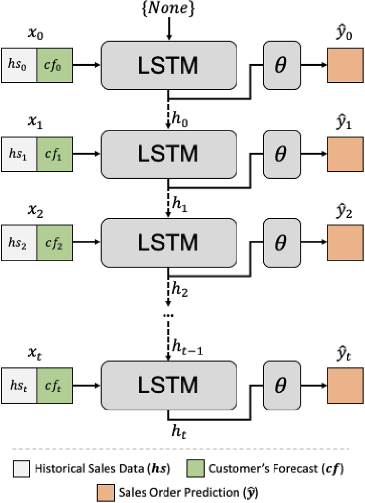
Fig. 2. The data-driven forecasting model uses both the historical sales data and the forecasts from customers as input for each time step.
B) Learning with Forecast Data
We choose LSTM for its ability to update and forget unwanted sequence information. As a data-driven approach, LSTM benefits from a large amount of data, exactly what the centralized ERP system can provide. To train the forecasting model, we use historical sales data in conjunction with forecasts from customers. When customers provide forecasts that overestimate the sales order amount, it can lead to high inventory costs. We find that customers can include non-market factors such as monthly sales targets or goals from promotional events. For that reason, we treat customer forecast as a hint to sales confidence, and it then becomes straightforward for us to integrate both historical sales data ($hs_{t}$ ) and forecasts from customers ($cf_{t}$
 ) as an input tensor, denoted by ${x_t = (hs_{t} \oplus cf_{t})}$
 , where $\oplus$
 represents the element-wise concatenate operation and $t$
 represents the time. The prediction $\hat {y_t}$
 is then

Here, $\theta$ represents fully connected layers that take in the activation of a LSTM network, and $h_{t-1}$
 denotes the temporal state from the previous time-step. During training, we use Adam optimizer to train $\theta$
 by minimizing:

In theory, it is possible to train a single forecasting model for all stock commodities. However, in practice, we found that training a single model that generalizes to multiple commodities with various sales patterns requires a substantial number of parameters and extensive effort. To make the training process tractable, we train commodity-specific forecasting models, and can successfully apply this data-driven approach to predict foreseeable customer demand.
C) Periodic Model Updates
Because of the periodic update nature of sales forecasts, we also update the model every time new sales data and forecasts are available. Because training a data-driven forecasting model requires a substantial computational resource, it is impractical to train the models in traditional ERP machine clusters without GPU. The problem then shifts to transferring sensitive data to another machine with more computational resources.
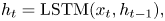
To create a secure connection between the ERP system and the training servers with GPUs, we set up an internal server that has access to the ERP system and a RESTful API (Figure 3). The API acts as a gatekeeper that moderates the data access to the ERP system – for example, retrieving data to train the forecasting model or displaying the latest sales order prediction.
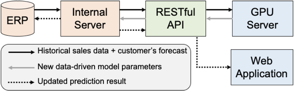
Fig. 3. Our system automatically update the data-driven forecasting model parameters through a RESTful API.
Every model update begins with the internal server querying data from the ERP system. The internal server then proceeds by sending the data to the GPU-accelerated machine through the API. Once the training process is complete, the GPU server sends new model parameters to the internal server. Finally, the internal server inferences the models and directly stores the predictions into the ERP system. For a better machine-to-machine translation, the predictions are in the form of CSV (Comma Separated Values) and JSON (JavaScript Object Notation).
D) Application Results
The customers may have adjusted the forecasts using their models before providing them to our manufacturing facilities with social listening, customer relationship management database, or historical order data for various manufacturing facilities. Therefore, it has been traditionally challenging to improve over the provided forecast as these data are not accessible by our factories. We have nonetheless achieved comparably higher accuracy with the data-driven forecasting model described in this section.
Figure 4 compares our approach to the customer's forecast and a classical forecasting algorithm, ARIMA. As expected, when we train the model once and never perform any update, it fails to capture sudden changes in sales patterns, which eventually leads to a higher error than the baselines provided by the customers. Using only the historical sales data, ARIMA provides a slight average improvement over the customer's forecast. In contrast, our approach uses both the customer's forecast and the historical sales data to make the sales prediction. With frequent model updates, our data-driven approach achieves the best prediction, reducing the forecast error by roughly 20% and making it a viable reference for logistic planning purposes. Regardless of the accuracy, the sales order prediction still needs corrections. In practice, because many physical and unrecorded factors change dynamically, our models’ prediction results are monitored and revised by experienced logistic planning personnel.
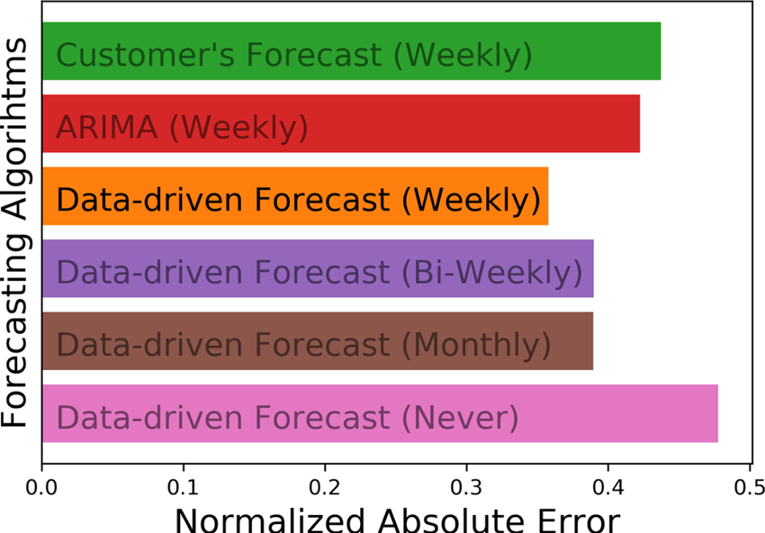
Fig. 4. Error comparison between our data-driven forecast model, customer's forecast, and ARIMA.
For the future, we would like to investigate ways to tackle the forecast of new commodities that have a smaller number of historical sales data compared to older commodities, such as using data from products with similar sales patterns [Reference Hu, Acimovic, Erize, Thomas and Mieghem18]. Another exciting direction is to forecast the raw materials by using hierarchical constraints [Reference Mishchenko, Montgomery and Vaggi19], where many finished goods may use the same raw materials.
IV. FUNCTIONAL VERIFICATION
There are three primary stages for the manufacturing of laptops, namely the production of circuit boards, machine assembly, and testing. Figure 5 shows several pictures of the assembly process. In a conventional production line, a worker performs relatively small tasks within short amounts of time for higher production throughput. In an assembly cell, a worker would instead be responsible for the entire assembly task, making this setup more suitable for producing a wider variety of lower volume products. Both types of assembly require the installation of the system software, followed by a run-in period of several hours to ensure compliance with the specifications provided by the customer. At any given moment, different types of products can occupy different parts of the assembly line based on the work order assignments.
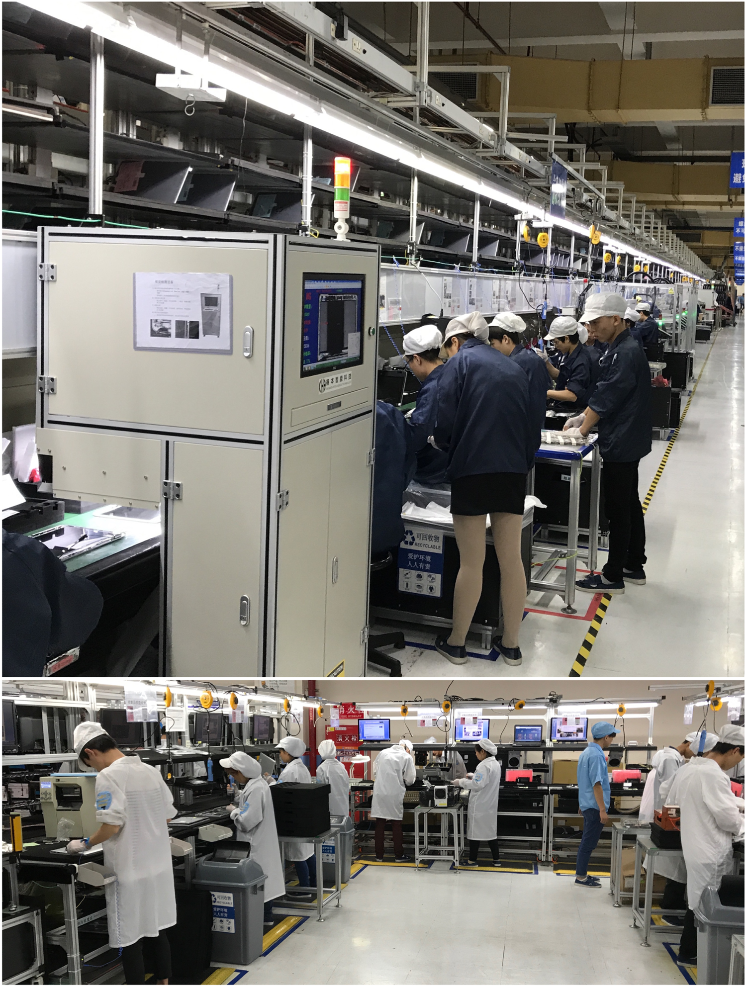
Fig. 5. A laptop system assembly facility. Top: an assembly line for higher production rate. Bottom: an assembly cell for lower yield but higher product variety.
While the automatic run-in period can resolve individual production issues, the process of verifying the correctness for each type of machine image remains a labor-intensive task marred with complicated processes that are prone to error. For example, a verification engineer may need to check the consistency of the version of the BIOS, which requires rebooting the machine several times. Each machine image takes more than 2 weeks to verify before it becomes ready for run-in deployment, and the confidence level for this highly manual process remains relatively low amongst the management team. For the specific facility we work with, there are over 200 verification engineers dedicated to the task of machine image verification alone, and clearly, the process can draw benefit from automation and computer vision technology.
A) The Testing Robot
To reduce the labor cost and boost confidence, the quality assurance team opts to replace humans with testing robots. To simplify the problem, we build a robotic keyboard with a configurable array of pneumatic actuators and attach it to the laptop. We use standard industry AOI cameras to receive visual feedback from the laptop screens, and control the cursor via the USB interface from a PC Workstation, which acts as a testing server. Figure 6 shows the overview of the system, and Figure 7 shows the physical implementation of our testing robot.
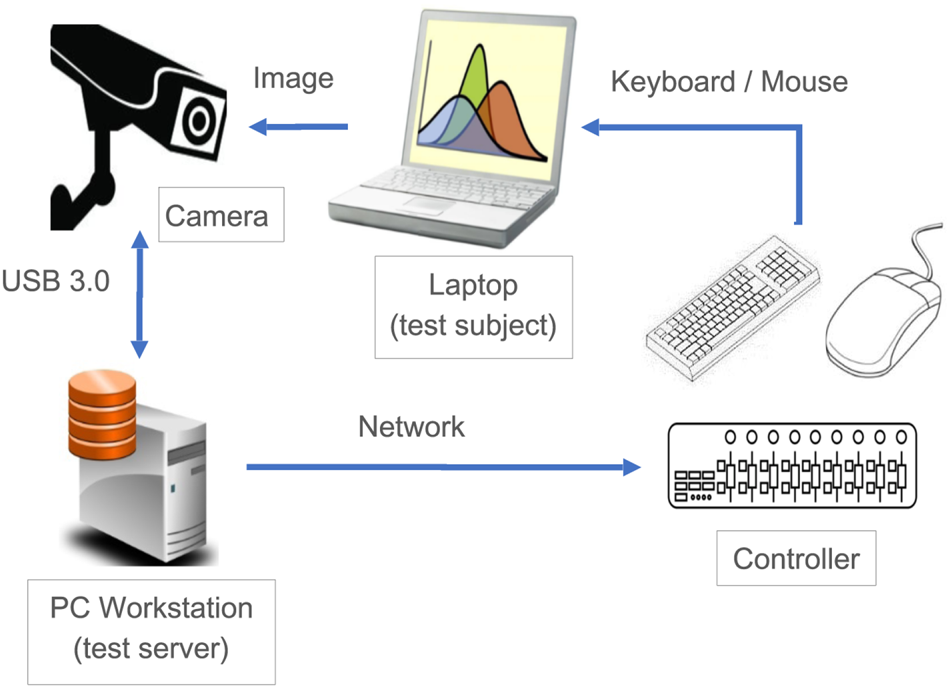
Fig. 6. The overview of the laptop functional testing system.
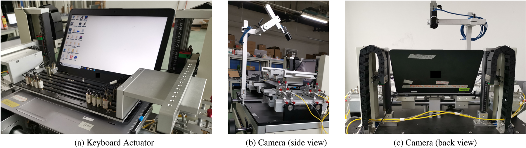
Fig. 7. (a) Keyboard Actuator. (b) Camera (side view). (c)Camera (back view). The production hardware for the function testing system.
For the testing robot to function correctly, it needs to be able to recognize the contents on the screen and perform actions according to the test scripts. For this purpose, we built a computer vision library with the following functionalities using a combination of open-source [Reference Bradski20, Reference Smith21] as well as routines developed in-house.
• Screen Calibration. Because we have calibrated the intrinsic parameters for the camera, we only need to find the edges and corners of the laptop screen in order to acquire the extrinsic transform between the camera and the screen. In practice, this requires the use of edge detection routines followed by a 2D homography transformation. The calibration process is performed once per test laptop and does not occur very frequently.
• GUI Localization. Often, a test script involves clicking an icon from the desktop, navigating the GUI, and typing correct keystrokes from the terminal. Because the robots operate without controlled lighting, the color profile and brightness on the screens may vary. Therefore, we adopt a denoising routine to clean up the input camera image, followed by a multi-scale template matching algorithm to locate the icons or GUI elements requested by the testing script. We can then actuate the mouse pointer through the USB controller interface to point and click on the elements, or activate the keyboard through either the USB controller or the robotic keyboard.
• Output Recognition. Execution results of the tests often come in the form of text. For this purpose, we use an LSTM-based OCR engine [Reference Smith21] to extract text information from the screen. To focus only on the interest regions of the screen, we adopt a two-step process. First, we locate user-specified GUI elements through localization. This extracted element then serve as anchors for computing the region of interest from the screen.
Figure 8 shows the testing robot in action, where the machine on the right is the test server responsible for driving the test subject on the left. Typical steps such as rebooting the system and running test programs can take up to several minutes, wasting valuable time by the verification engineers. Our system can execute these steps through keyboard and mouse controls, detect the steps’ completion through the camera, and record the results onto the spreadsheet on the testing server. Please refer to the video talk in [Reference Chen and Chen22] for a complete example of the test execution process.
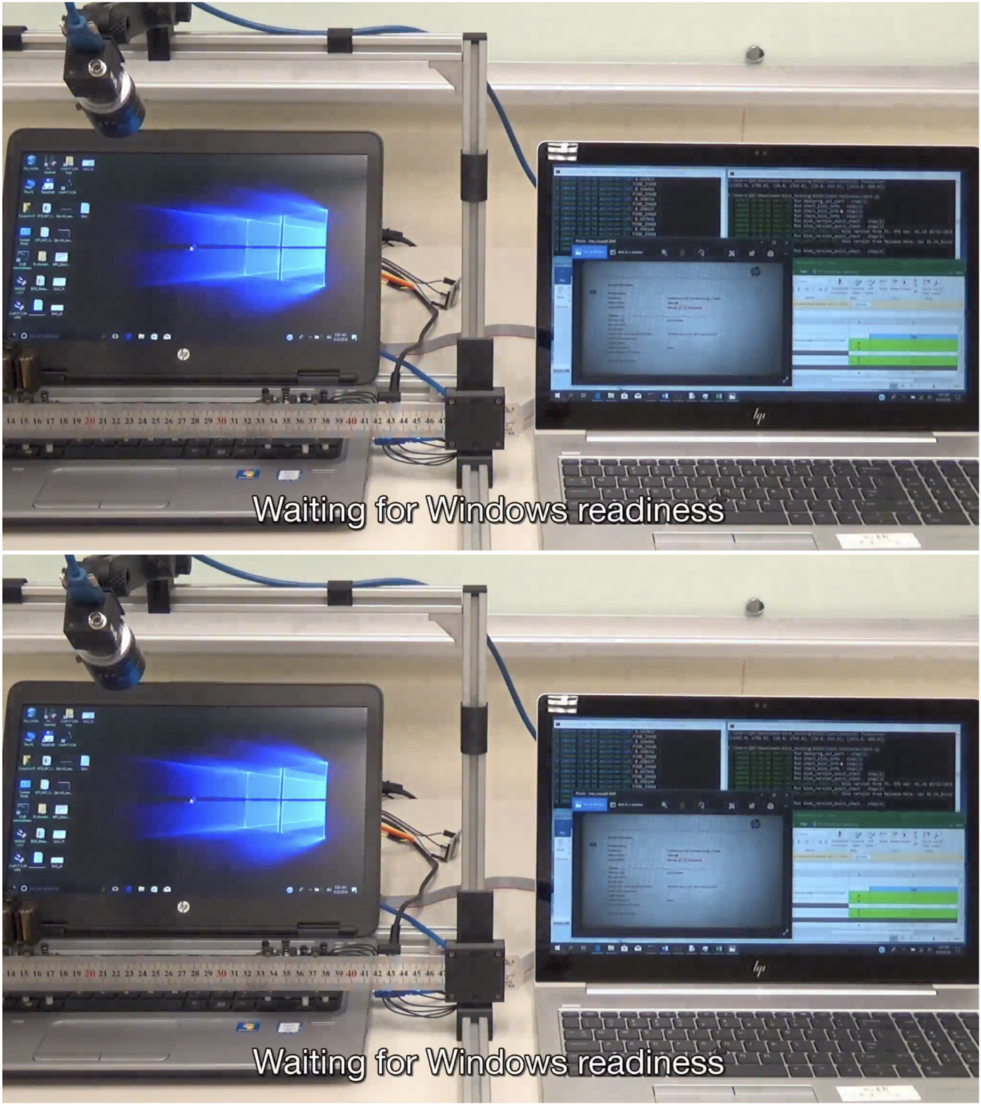
Fig. 8. Several typical test steps and their screen shots.
B) Managing Test Case Complexity
The test cases are stored either locally on the workstation, or more often on a remote testing server so that each workstation receives the most up-to-date version of the testing scripts. All in all, the number of test cases in the scope is close to a million, which makes implementing and maintaining the test cases a rather daunting task. To make this more tractable and reduce the combinatorial explosion of testing scripts, we identify common sub-scripts and use them to form a basis to reconstruct the full scope of tests.
Additionally, to ensure timely implementation of the test cases, we adopt standard programming languages such as Python as the baseline for the test scripts and add additional language constructs for our parser to recognize the parts of instructions specific to the control of the testing robots. We found that, compared to the use of custom scripts with recorder interface [Reference Cheng, Kuo, Cheng and Kuo23–Reference Lee, Chen, Ma and Lee25], the use of familiar programming languages allow us to scale up the development effort, both on-site or remotely, so that the overall development time for the scripts lasts a relatively manageable timeframe of 18 months.
Also, while the logic of the testing scripts remains the same, the appearance of GUI elements or icons may change over time because of operating system software updates. For this, we enhance our GUI Localization routine to include multiple scales and versions of the same element to improve the robustness of localization.
C) Practical Impact
With the introduction of the automated testing robot in the functional verification workflow, we have managed to reduce the number of active verification engineers by over half, which translates to hundreds of people. The number of projects handled by the factories has also increased during the period. Since this is the only process improvement we have implemented for functional verification, it is a direct quantitative proof that this system has dramatically reduced our verification labor costs. Its direct impact is estimated to be 150 person-year of labor reduction and two million US dollars of cost reduction per year in one factory alone.
In terms of management confidence, their additional commitment to invest and deploy the system serves as a qualitative proof for the impact of the project. Before introducing automation, multiple verification engineers may be running on the same set of tests separately. This workforce redundancy is similar to the problem exhibited with unreliable workers [Reference Ipeirotis, Provost and Wang26], and is an extra cost that business units have to bear. The robots, with their high repeatability, can serve as high-quality workers to augment human engineers. The resulting workforce reduction is another qualitative testament to improved management confidence.
V. APPEARANCE INSPECTION
Appearance inspection is essential on assembly lines because undetected defects can be costly in terms of parts waste, product returns, and loss of customer trust. The rapid advancement of automation technology enables more sophisticated equipment for manufacturing, leading to larger volumes of production at significantly shorter production cycle time. On the other hand, appearance inspection largely remains a labor-intensive process, where human inspectors are often required to visually qualify each product against the acceptance criteria such as the number of acceptable scratches, dents, and area of these defects, all within tens of seconds. This labor-intensive process is prone to human errors due to factors such as environmental conditions, distractions, and fatigue, making it challenging to maintain a consistent standard for inspection. Existing automatic inspection systems are primarily rule-based systems using traditional computer vision techniques [Reference Steger, Ulrich and Wiedemann27]. These systems can check against manually designed rules for specific purposes, such as whether the logo is in place through template matching [Reference Crispin and Rankov28] or the presence of contours or holes through edge detection and shape models [Reference Steger, Ulrich and Wiedemann27]. While these systems perform well for specific visual checks, they do not have the flexibility and adaptability of human inspectors to detect defects outside of the programmed rules. Often, it becomes too expensive and time-consuming to deploy sufficient rules for a large variety of products because of the significant manual engineering efforts involved in writing rules for every type of defect checks.
Ideally, we want an automatic inspection system that can reduce the amount of engineering and time required to deploy the system and that leads us to learning-based methods that are adaptable to any products by automatically learning these rules in a data-driven fashion. We describe our experiences in employing fully supervised object detection-based models (Section V.A), as well as our transition to unsupervised auto-encoders (Section V.B)) to address the limitations of object detectors.
A) Supervised Defect Detection
An automatic inspection system should be able to determine whether a product passes the acceptance criteria and localize the defects for us to verify its predictions. A natural choice would be to use a deep learning-based object detector that takes in an input product image and outputs bounding boxes around candidate defect regions. We first share our experiences regarding annotating defects, followed by details of the object detection model. Lastly, we discuss how we decide whether a product passes the acceptance threshold given the defect regions.
1) Annotating defects
In order to train an object detection model, we need to collect examples of defective products and annotate the defects with bounding boxes and labels. The quality of our labeled training data and its representation heavily affect the performance of the detection model. Based on our experience, collecting and annotating defect data requires several additional considerations compared to natural images. For example, the defect classes, or types, are not clearly defined, making it difficult to provide simple instructions for the annotators. Also, defects can appear anywhere and take on all forms, shapes, and sizes. Figure 9 shows some examples of defects we encountered, and we discuss these common challenges for annotating defects below. As a result, we find it a significant effort to enforce a consistent annotation standard, which is crucial for training and evaluating our models.
• Ambiguous defects. Defects may appear differently on different product surface textures, making their class assignment ambiguous. For example, in Figure 9(b), the dotted textures that form lines similar to scratches can be individual small scratches for one annotator, and a complete dotted line for another.
• Unexpected defects. During the annotation process, there will be cases of rare defects that do not belong to any of the defect types listed in the annotation guidelines. Figure 9(b) shows one such example with an accidentally placed sticker on the laptop.
• Grouping of defects. Disconnected defects are difficult to group. For example, we can see in Figure 9(c) an example of a scratch that was caused by a single stroke, but there are gaps in the middle of the scratch. Do we consider them multiple scratches or just a single scratch?
• Tightness of the bounding box. For some defects, the tightness of bounding boxes heavily affect the performance of the model. Figure 9(d) shows an example of varying tightness of bounding box annotations. Our initial intuition favors tighter bounding boxes with less background information. However, in practice, we find the background information to be essential for classifying the patches, particularly when the defects are circular or rectangular.
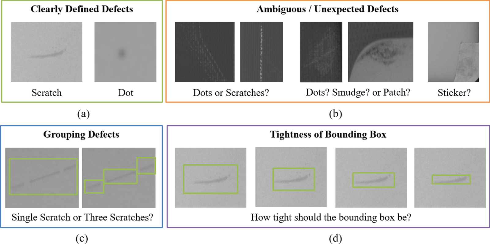
Fig. 9. Some examples of defects. (a) Defects that are clearly defined and easily recognizable. (b) Ambiguous or unexpected defects that are confusing to annotate. (c) Defect sample that illustrates the confusion in grouping defects. (d) Varying tightness of the bounding box.
2) Detection model
For the object detection model, we employ Faster-RCNN [Reference Ren, He, Girshick and Sun29], which is known to be a relatively fast and accurate detector. It consists of three components: a feature extractor network, a region proposal network, and a refinement network (Figure 10). The feature extractor network – also referred to as the backbone network – is responsible for learning meaningful feature representations of the input image. It outputs a tensor with a lower spatial resolution, where each spatial location is a vector that encodes features of a corresponding patch in the input image. This information bottleneck forces it to extract only the most useful information for the task. Its convolutional neural network is pre-trained on a classification task such as ImageNet classification. Since classification and object detection are two closely related tasks, the features extracted by the classifier network also work for detection. Common architectural choices include VGG [Reference Simonyan and Zisserman30] architecture or the ResNet [Reference He, Zhang, Ren and Sun31] architecture.

Fig. 10. Overview of the Faster-RCNN pipeline.
The region proposal network outputs a set of bounding box proposals corresponding to candidate locations on the image that may contain defects. We represent a bounding box as a set $\{\hat {p_x},\hat {p_y},\hat {w},\hat {h}\}$ , where $\hat {p_x}, \hat {p_y}$
 represent its coordinates and $\hat {w},\hat {h}$
 represent its width and height, respectively. These candidate bounding boxes and their related anchor boxes act as prior knowledge on the sizes of objects found in the dataset, allowing the network to output boxes of different scales and sizes since it only has to learn the relative modifications from the anchor boxes.
Each candidate bounding box comes with a confidence score of $s$ ranging from $0$
 to $1$
 , indicating how likely it is to contain a defect. This score allows us to rank and filter the bounding boxes according to a pre-defined threshold. At this stage, we use a relatively lower threshold to increase the chances of capturing the defects. The region proposal network optimizes for two losses: the bounding box regression loss $L_{bbox}$
 that minimizes the difference between the ground truth box and the predicted box defined in Eq. 1, where the variables with $w_a$
 and $h_a$
 are width and height of an anchor box, and the score loss $L_s$
 , which is a standard binary cross-entropy loss defined in Eq. 2, where $y$
 is a ground truth label indicating whether the box contains a defect or not.


Finally, the refinement network further refines the estimates from the region proposal network. It extracts the feature tensors corresponding to the area defined by the candidate bounding boxes, and performs region of interest alignment (roiAlign) [Reference He, Gkioxari, Dollár and Girshick32] to resize the feature tensors to a pre-defined spatial resolution. These resized tensors enter a series of convolutional layers to produce a set of refined bounding boxes with adjusted defect scores.
3) Acceptance model
While the detector identifies and locates defects, we are ultimately interested in a binary pass-or-fail decision. To achieve this, we use a support vector machine (SVM) on top of the features extracted by the object detector combined with handcrafted features such as the area of defects, counts of defects, and discrete cosine transform features. The SVM essentially learns customer-specified acceptance criteria from examples of products that passed the quality assurance, as well as those that failed. Moreover, we can easily change the threshold for classification to classify the quality of the product, making the entire pipeline adjustable for quality control purposes.
B) Unsupervised Defect Detection
In a production line, the majority of products will be normal since manufacturers will actively try to reduce the factors that cause defects. That means the availability of defect images tends to be rare and insufficient for the object detector to learn. The imbalance of training data amongst different defect classes also makes training sub-optimal. It generally takes several months to gather sufficient labeled images to achieve reasonable accuracy, which can be impractical considering the relatively short life-cycle of products.
To remove the significant bottleneck of collecting and annotating defects, we seek to learn from normal data, which are abundant and require no labeling or tagging. Following this line of thought, we employ auto-encoders [Reference Gong, Liu, Le, Saha, Mansour, Venkatesh and Hengel33–Reference Zong, Song, Min, Cheng, Lumezanu, Cho and Chen35] to learn and memorize only normal data (Section V.B).B.1) and treat everything that deviates too far from normal as defects (Section V.B).B.2).
1) Auto-encoder model
An auto-encoder is effectively a compression algorithm where an encoder network learns a coded representation of the input, and a decoder network reconstructs an output from this code similar to the original input (Figure 11). We achieve this goal by minimizing the mean squared error between the input $x$ and the reconstruction $\hat {x}$
 , as shown below,
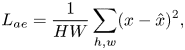
where $H,W$ denote the height and width of the input image. Forcing the code to a lower dimension then the input enables the encoder to extract only the most essential features necessary for reconstruction.
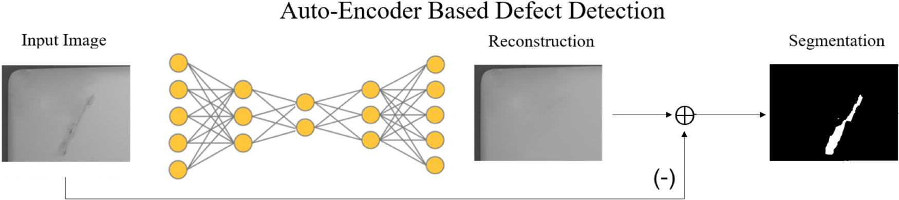
Fig. 11. Overview of the Auto-Encoder pipeline for defect detection.
Unlike standard compression algorithms, auto-encoders learn features specific only to the data corpus, which means it can only reconstruct data within this training distribution. We exploit this property for defect detection wherein we train the auto-encoder only with normal data. This auto-encoder will then have problems reconstructing abnormal inputs, allowing us to separate defects from the images.
2) Separating defects
As discussed earlier, parts with larger reconstruction error from the auto-encoder provide hints to the location and region of the defects. In order to separate defects from normal, we must first define a segmentation threshold of $\delta$ . Applying this threshold on the reconstruction error map as follows,
we get a binary segmentation mask $M\in \mathbb {R}^{H \times W}$ that has a value of one for defective regions and zero for normal regions.
3) Acceptance model
Similar to the object detector, we also convert the output from the auto-encoder to a binary pass-or-fail decision. Given the segmentation mask $M$ , we extract connected regions using a flood fill algorithm, followed by fitting a bounding box around each region. Then we can employ the same SVM process to decide whether the input is acceptable or not.
C) Defect Detection in Practice
Figure 12 shows a photo of our custom-built machine for automatic inspection of laptops. It automatically pushes a laptop out of the conveyer belt and uses multiple cameras to take pictures in parallel, capturing all sides of the laptop with actively controlled lighting. The specifications of the machine are listed below:
• Machine size ($L \times W \times H$
 ): $160 \times 100 \times 200 cm^3$
• Power requirement: 6000W / 220V
• Machine weight: 520 kg
• Camera sensor type: CMOS
• Camera maximum resolution: 10000 x 7096 pixels
• Acceptable laptop size: 12***** to 17*******


Fig. 12. Snapshot of our machine for automatic inspection of laptops.
1) Algorithm details
We initialize the Faster-RCNN model with pre-trained weights from MS-COCO[Reference Lin, Maire, Belongie, Hays, Perona, Ramanan, Dollár and Zitnick36] and trained for 30 epochs on our target dataset using only a few labeled data. For the auto-encoder, we train it for 100 epochs on an unlabeled dataset containing mostly normal images. All networks are optimized using stochastic gradient descent (SGD) with momentum 0.9, weight decay 0.0001, and an initial learning rate of 0.001. We augmented our dataset using random horizontal flips except for products where orientation is important.
2) Datasets
We experimented with these models on a proprietary laptop dataset, two publicly available datasets, namely DAGM [Reference Arbeitsgemeinschaft für Mustererkennung (DAGM), D37], and MVTec [Reference Bergmann, Fauser, Sattlegger and Steger38]. The DAGM [Reference Arbeitsgemeinschaft für Mustererkennung (DAGM), D37] dataset was originally for a competition on weakly-supervised learning for industrial optical inspection. It consists of synthetic textures with various types of defects. The MVTec [Reference Bergmann, Fauser, Sattlegger and Steger38] dataset, on the other hand, contains a diverse set of real-world products for industrial inspection.
3) Results and discussion
In an actual manufacturing setting, rare and unexpected defects can occur. An example of this is the tape shown on the left side of Figure 13.
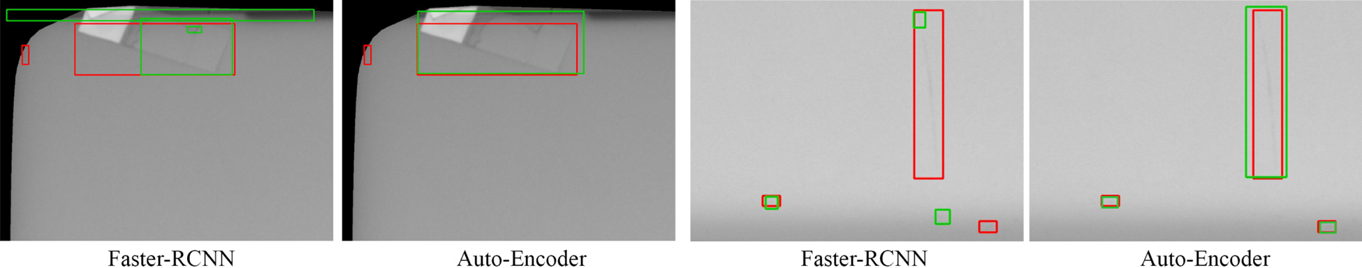
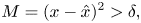
Fig. 13. Visual results of Faster-RCNN compared to the Auto-Encoder for defect detection on laptop surfaces. We converted the segmentation results from the auto-encoder into bounding boxes for easier comparison. Red boxes show the ground truths; green boxes show the predictions.
The nature of the data distribution poses significant latency in collecting and labeling the data, as even domain experts would have difficulty producing accurate labels, as discussed in our talk in [Reference Chen and Chen39]. Faster-RCNN [Reference Ren, He, Girshick and Sun29] will have difficulty detecting this type of defect since it does not appear in any of the training images. In contrast, the auto-encoder can successfully detect the entire defect since the appearance is very different from a normal laptop's surface. On the right side of Figure 13, Faster-RCNN failed to capture the long scratch, which may be due to the dataset having mostly smaller defects.
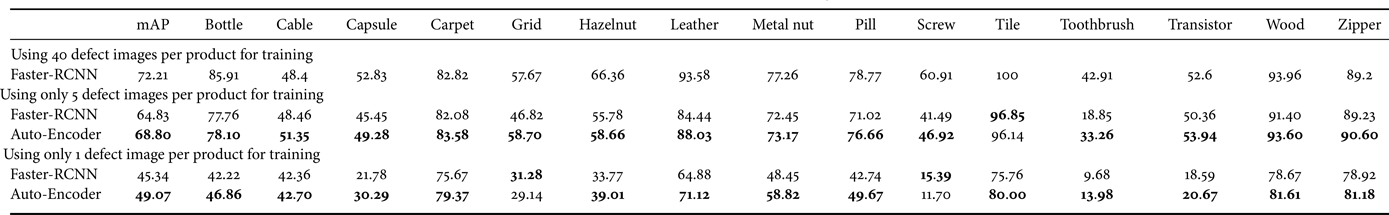
Figure 14 shows example results of Faster-RCNN and auto-encoder trained on only five defect samples from the DAGM and MVTec dataset. Note that we converted the segmentations of the auto-encoder into bounding boxes to make it easier to compare with Faster-RCNN. Since the object detector is trained on very few defect data, it could not capture many of the defects that it did not see during training. In contrast, the auto-encoder can successfully detect and localize these defects.

Fig. 14. Visual results of Faster-RCNN compared to the Auto-Encoder for defect detection on DAGM (top) and MVTec (bottom) datasets, given only on five defective image samples per product for training. We converted the segmentation results from the auto-encoder into bounding boxes for easier comparison. Red boxes show the ground truths; green boxes show the predictions.
In particular, because our auto-encoder includes a design where we can control the latent space's conditional entropy, it allows us to balance between generality and specificity of the model to avoid reconstructing defects [Reference Chen and Chen39].
We also use the average precision (AP) to evaluate the localization performance across all possible thresholds. Table 1 shows the results of each product type in the DAGM dataset. Faster-RCNN trained on all the labeled defects achieve almost a perfect score. However, when we reduce the number of labeled defects, its performance also drops. The auto-encoder approach surpasses the Faster R-CNN baseline by up to 12.89% mAP in the one defect sample setting, and 1.39% mAP in the five defect setting.
Table 1. Results on the DAGM dataset in terms of average precision (AP).
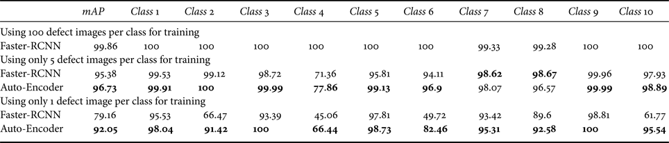
Similarly, Faster R-CNN performs well on the MVTec dataset when trained with many labeled defects, achieving a mean average precision (mAP) of 72.21%. In the small labeled defect setting, the auto-encoder outperforms Faster-RCNN with a 3.73% mAP increase in the one defect setting, and a 3.97% mAP increase in the five defect setting, as shown in Table 2.
Table 2. Results on the MVTec dataset in terms of average precision (AP).
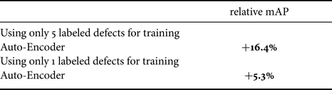
For the proprietary laptop dataset, we can report only the relative differences between our auto-encoder method and the Faster-RCNN baselines due to confidentiality reasons. Observe in Table 3 that our auto-encoder achieves a 16.4% mAP increase over Faster-RCNN with only one labeled defect and 5.3% mAP increase with five labeled defects. The result shows that auto-encoders can reduce the number of manual annotations and compares favorably to the fully supervised Faster-RCNN, making it desirable for detecting defects, especially during the early stages of production.
Table 3. Results on the proprietary laptop dataset compared to the Faster-RCNN baseline.
VI. CONCLUSION
The transformation from automation to smart manufacturing is an evolutionary process. The projects presented here all derive real effects from parties involved, paving the road to their full-scale adoption in our facilities. Per company policy, we can not disclose the immediate effects of these projects. Suffice to say that the continual commitment, both in development and process adaptation, proves their usefulness for all stakeholders involved. For the future, in addition to improving the accuracy and performance of our algorithms, we are in the process of implementing a more thorough digital twin and data policy to discover additional opportunities within the manufacturing facilities. Projects such as the logistic management are considered core to the business and can only be used exclusively by the company. Others, such as appearance inspection, can create new revenue streams without hurting the company baseline, and we are actively seeking opportunities for sharing these solutions to our peers.
Many people helped with various aspects of the projects in this article. To comply with company policy, we shall not reveal their full names here. For the functional testing project, we wish to thank Jimmy for implementing the first version of the testing server; Eric, Joseph, and Jack and the rest of the QA team for providing valuable input, building the testing robot, and steering the effort for managing test cases. We wish to thank our friends from the factory for providing training images for the AI models; Steven, Jerry, and his team for building the first version of the appearance inspection machine; our external collaborators for designing the next version of the machine; Anderson and Sean for facilitating the certification of the machine; Kristy and Josh for organizing the image annotations efforts. Steve and Mark and our IT department have been instrumental in helping us bridge the data necessary for the logistic management project; our logistic experts have been beneficial at educating the rest of us on the existing process. Finally, we wish to thank Jade and the technical committee for tirelessly coordinate many of the tasks behind the scene to make things happen.
Yi-Chun Chen is an AI Research Engineer at Inventec Corporation. Her research interests include deep learning and computer vision, especially object detection and metric learning, and their applications to smart manufacturing. Previously at Viscovery, Yi-Chun has developed visual search solutions for smart eCommerce. She received her BS from National Tsing-Hua University. Her publications include 360-degree vision, image captioning, and wearable vision system.
Bo-Huei He is a backend developer at Skywatch Innovation. He is a crucial member in the development of various video streaming and computer vision applications at Skywatch. His interests are in cloud computing, computer vision, system development, and AI.
Shih-Sung Lin is an IoT Developer at Skywatch Innovation. His research interests involve Internet-of-Things, embedded systems, AI, and computer vision. He developed several IoT services for Skywatch Innovation. He received his BS in Electrical Engineering from National Taipei University of Technology (2013), and BS in Networking and Multimedia from National Taiwan University (2015).
Jonathan Hans Soeseno is an AI Research Engineer at Inventec Corporation, where he applies deep learning, signal processing, and computer vision for industrial tasks. His research interests involve generative models, image processing, and computer vision. He received his B.Eng in computer engineering from Petra Christian University, Indonesia (2017), and MS in computer science from the National Taiwan University of Science and Technology (2018).
Daniel Stanley Tan works as an AI Research Engineer at Inventec Corporation, where he applies deep learning and computer vision techniques for industrial tasks. His research mainly focuses on generative models for smart manufacturing and precision agriculture. He is currently pursuing his Ph.D. degree at the National Taiwan University of Science and Technology. Before this, he held a faculty position at De La Salle University, Philippines.
Trista Pei-Chun Chen is the Chief Scientist of Machine Learning at Inventec Corp. Her research interests include machine learning and computer vision, especially their applications in smart manufacturing, smart health, medical AI, multimedia big data, and multimedia signal processing. Previously, Trista led a startup that was later acquired, was part of the Intel OpenCV development team, and architected Nvidia's first video processor. She received her Ph.D. from Carnegie Mellon University and MS and BS from National Tsing Hua University.
Wei-Chao Chen is a co-founder and the Chairman at Skywatch Innovation, a provider for cloud-based IoT and video products. He is also the Head of the AI Center and Chief AI Advisor at Inventec Corp. His research interests involve graphics hardware, computational photography, augmented reality, and computer vision. Dr. Chen was an adjunct faculty at the National Taiwan University between 2009 and 2018, a senior research scientist in Nokia Research Center at Palo Alto between 2007–2009, and a 3D Graphics Architect in NVIDIA between 2002–2006. Dr. Chen received his MS in Electrical Engineering from National Taiwan University (1996), and MS (2001) and Ph.D. (2002) in Computer Science from the University of North Carolina at Chapel Hill.


 Open access