
I. INTRODUCTION
In the world of digital signal processing (DSP), there are three fundamental tools that have become the basis of every algorithm, system, and theory dealing with the processing of digital audio. Those are the Nyquist sampling theory, the Fourier transform, and digital filtering. We could add a fourth one – the short time Fourier transform – which generalizes the Fourier transform to account for non-stationary signals such as music and speech. These concepts are so embedded into the creative thinking of audio engineers and scientists that new ideas are often intuitively based on one (or more) of these fundamental tools. Digital audio coding, speech synthesis, and adaptive echo cancellation are great examples of complex systems built on the theories of sampling, Fourier analysis, and digital filtering.
Fourier theory itself is built on some of the most basic tools of mathematics, such as vector spaces and integration theory (although harmonic analysis was not originally conceived this way by Joseph Fourier [Reference Fourier1]). From an intuitive perspective, the Fourier transform can be seen as a change of representation obtained by projecting the input signal s(t) onto an orthogonal set of complex exponential functions φ(ω,t) = e
−jωt
, given by $S\lpar \omega\rpar = \vint_{\open R}s\lpar t\rpar \varphi\lpar \omega\comma \; t\rpar dt$
. The Fourier representation is useful for many types of signals, and is oftentimes the logical choice. As a consequence, many of the mathematical and computational tools available today for the purpose of DSP have been developed under the assumption that the input signal is processed in the Fourier domain.
$S\lpar \omega\rpar = \vint_{\open R}s\lpar t\rpar \varphi\lpar \omega\comma \; t\rpar dt$
. The Fourier representation is useful for many types of signals, and is oftentimes the logical choice. As a consequence, many of the mathematical and computational tools available today for the purpose of DSP have been developed under the assumption that the input signal is processed in the Fourier domain.
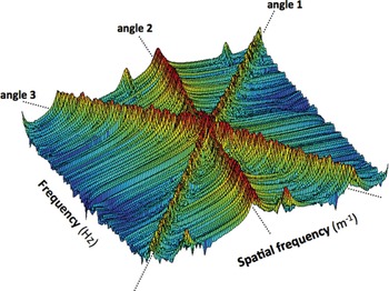
2D Fourier spectrum of an acoustic wave field generated by three far-field sources.
In digital audio, the fact that the Fourier transform kernel e jω t is an eigenfunction of linear time-invariant systems makes it a natural choice for representing sound signals in time. In this paper, we explore the assumption that the Fourier transform is a natural choice for representing sound fields in both space and time.
The concept of “spatial dimension” of an audio signal dates back to the development of array signal processing. The underlying principles are similar to those of electromagnetic antennas: an array of sensors (microphones) samples the wave field at different points in space, and the combined signals are used to enhance certain features at the output. Beamforming and source separation [Reference Van Veen and Buckley2, Reference Veen3] – two widely used techniques – are forms of spatial filtering. On the reproduction side, the idea translates as follows: an array of transducers (loudspeakers) positioned at different points in space synthesize the acoustic wave front from a discrete set of spatial samples. Techniques that use this principle include Ambisonics [Reference Gerzon4], near-field higher-order Ambisonics [Reference Daniel, Nicol and Moreau5], Wave Field Synthesis (WFS) [Reference Berkhout6, Reference Berkhout, de Vries and Vogel7], Spectral Division Method [Reference Ahrens and Spors8], and Sound Field Reconstruction [Reference Kolundžija, Faller and Vetterli9].
Arrays of audio transducers enable the sound field to be sampled and reconstructed in space just like a sound signal is sampled and reconstructed in time. On the one hand, recent advances in acoustic sensing technology [Reference Neumann10] have made microphones small enough such that the sound field can be sampled in space at the Nyquist rate.Footnote 1 Since the sound field is typically band-limited, as we will see later, this means it can be sampled and reconstructed with little spatial aliasing. On the other hand, the ground-breaking work on wave field synthesis [Reference Berkhout6] has made it possible to think of loudspeakers as interpolation points in a synthesized wave front, just like digital samples that reconstruct an analog signal. As a result, the sound field can be conveniently interpreted as a multidimensional audio signal with a temporal dimension and (up to) three spatial dimensions. Such a signal can be processed by a computer using multidimensional DSP theory and algorithms.
The goal of this paper is not to build on the theory of acoustics, nor present competing sound field processing and rendering techniques, but rather to provide an intuitive view of how the three fundamental tools of DSP translate into the world of digital acoustics, where audio signals have both temporal and spatial dimensions, and are sampled in both of them. We show what it means to sample and reconstruct a sound field in space and time from the perspective of signal processing, and what the respective Fourier transform is. With a proper understanding of the spectral patterns caused by each source in the acoustic scene, it becomes easy and intuitive to design filters that target these sources. It also provides a framework for the design of discrete space and time algorithms for sound field processing, including sound field rendering, filtering, and coding.
II. ACOUSTIC SIGNALS AND THE WAVE EQUATION
When we think of an audio signal – or an acoustic signal – having a spatial dimension, we need to move our framework into a multidimensional space. Depending on the number of spatial dimensions considered, the signal can have between two and four independent variables. For simplicity, we will consider only one spatial dimension, although the theory can be extended to all three dimensions. Our signal will then be a function p(x, t), where x is the position along the x-axis and t is the temporal dimension.
Signals defined in such a way belong to a particular class of signals, in the sense that p(x, t) must satisfy the wave equation. Points in the function are not independent, but rather tied by a propagating function. Unlike images, acoustic signals are not direct two-dimensional (2D) extensions of traditional 1D signals. Namely, while in digital image processing the x and y dimensions are interchangeable, in acoustics the x and t dimensions are linked (or correlated) through the wave equation.
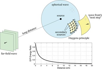
The essentials of acoustic signal processing are based on three core principles of theoretical acoustics: (i) spherical radiation [Reference Morse and Ingard11], (ii) modes of wave propagation [Reference Williams12], and (iii) the Huygens principle [Reference Morse and Ingard11]. Each of these principles, which can be derived from the wave equation, is associated with a different stage of a DSP system. Spherical radiation is relevant to the analysis of acoustic signals in space and time. The modes of wave propagation are visible in the Fourier domain, and they affect the spectral patterns generated by the acoustic wave fronts. The Huygens principle provides a basis for interpolation of a sampled wave front. These three principles, illustrated in Fig. 1, are described in more detail bellow.
An illustration of the three physical principles: (i) a point source generates a spherical wave front, which becomes increasingly flat in the far-field; (ii) as the distance increases, the ratio between evanescent energy (E) and propagating energy (P) decays to zero; (iii) the Huygens principle implies that the wave front is a continuum of secondary sources that generate every “step” in its propagation.
A) Spherical radiation
Spherical radiation is the radiation pattern generated by point and spherical sources in open space. A point source is an infinitely compact source in space that radiates sound equally in all directions, giving the wave front a purely spherical shape. Many sound sources can be modeled as point sources, or as systems comprising multiple point sources – the so-called multipoles. Reflections caused by walls in a closed space can be equally interpreted as virtual point sources [Reference Allen and Berkley13]. This suggests that a description of the acoustic scene solely based on point sources can be accurate enough to characterize the resulting wave field.
In the particular case when the source is located in the far-field, i.e., at a long distance from the observation region, the incoming waves appear to have a flat wave front characterized by a direction of propagation. The two types of radiation are illustrated in Fig. 1.
Plane waves show up in the steady-state analysis of the wave equation in Cartesian coordinates [Reference Williams12], and represent simple-harmonic sound pressure disturbances that propagate in a single direction (thus they have planar wavefronts). We will see that the plane wave is the elementary component in the spatiotemporal Fourier analysis of a wave field, the same way complex frequencies are the elementary components in traditional Fourier analysis. The local characteristics of the wave field converge to a far-field case as the observation region moves away from the source (and vice versa), and this happens already a few wavelengths away. This is the main motivation for the use of space–frequency analysis, addressed later in the paper.
Note, however, that far-field waves in the free field are an idealization, since their amplitude does not decay with the distance – something not possible under the Sommerfeld radiation condition given by (2), as described in Box II.1.
Spherical Radiation
The wave equation in Cartesian coordinates is given by
 $$\left(\nabla^{2} - \displaystyle{1 \over c^2} \displaystyle{\partial^2 \over \partial t^2} \right)p\lpar {\bf r}\comma \; t\rpar = -f\lpar {\bf r}\comma \; t\rpar \comma \;$$
where, for an acoustic wave field, p(r, t) denotes sound pressure at the point of observation r = (x, y, z) and time t. The Laplacian operator ∇Reference Van Veen and Buckley
2
is given by $\nabla^{2} = \displaystyle{\partial^2 \over \partial x^2} + \displaystyle{\partial^2 \over \partial y^2} + \displaystyle{\partial^2 \over \partial z^2}$
, and the speed of sound is given by c in m/s. The function f(r, t) describes the source of radiation, and is a function with compact support.
$\nabla^{2} = \displaystyle{\partial^2 \over \partial x^2} + \displaystyle{\partial^2 \over \partial y^2} + \displaystyle{\partial^2 \over \partial z^2}$
, and the speed of sound is given by c in m/s. The function f(r, t) describes the source of radiation, and is a function with compact support.
A solution to (1) that corresponds to radiating sound sources needs to satisfy the Sommerfeld radiation condition given by [Reference Williams12]
 $$\lim_{r \rightarrow \infty} r \left[\displaystyle{\partial \over \partial r} - jk \right]p\lpar {\bi r}\comma \; t\rpar = 0\comma \;$$
where r = ‖ r ‖, k = ω/c is the wave number, and ω the temporal frequency.
In the case of a point source, the source can be simply described by f(r, t) = δ(r)s(t), where δ( r ) is a Dirac delta function and s(t) is the source signal at the singularity point. If the point source is at r p = (0,0,0) and in open space, the solution to (1) is given by [Reference Morse and Ingard11]
 $$p\lpar {\bf r}\comma \; t\rpar = \displaystyle{s\left(t - \displaystyle{r \over c} \right)\over 4\pi r}\comma \;$$
which represents the spherical radiation pattern.
In the far-field, the assumption is that r≫1/k. By applying it to (3) and normalizing the amplitude to 1, the result is given by
 $$p\lpar {\bf r}\comma \; t\rpar = s\left(t + \displaystyle{{\bf k} \cdot {\bf r}\over c} \right).$$
The wave vector k = (k x , k y , k z ) represents the direction of arrival of the flat wave front, and · denotes dot product. The most distinctive aspect of this result is that the sound pressure is dependent only on the direction of propagation of the wave front. In the case where s(t) = e jω0 t , the function p(r, t) is called a plane wave with frequency ω0 rad/s.
It should also be noted that in some applications the far-field conditions are not met, primarily at low frequencies. As a consequence, one needs to account for the near-field effects. Examples where this happens include near-field higher-order Ambisonics [Reference Daniel, Nicol and Moreau5] and near-field beamforming [Reference Ryan and Goubran14].
B) Modes of wave propagation
The convergence from spherical to far-field radiation is related to the concept of modes of wave propagation. A far-field acoustical wave front is not physically possible in the free field because it contains only one mode of wave propagation, called the propagating mode (PM). To satisfy the wave equation, the wave front must contain two modes of wave propagation: (i) the PM, which is responsible for the harmonic motion, and (ii) the evanescent mode (EM), which is responsible for the amplitude decay (see Box II.2 for more details). The ratio between the two modes depends on the distance from the point source to the region of observation and the wavelength λ. The plot in Fig. 1, which shows the normalized ratio between EM and PM for one temporal frequency, shows that the energy contribution of the EM decays to zero exponentially.
Modes of wave propagation
Plane waves are simple-harmonic functions of space and time obtained as the steady-state solutions of the homogeneous acoustic wave equation in Cartesian coordinates [Reference Morse and Ingard11],
 $$\displaystyle{\partial^2p \over \partial x^2} + \displaystyle{\partial^2p \over \partial y^2} + \displaystyle{\partial^2p \over \partial z^2} - \displaystyle{1 \over c^2}\, \displaystyle{\partial^2p \over \partial t^2} = 0.$$
They are expressed as analytic functions of the spatial coordinate r = (x,y,z) and time t,
 $$p\lpar {\bi r}\comma \; t\rpar = P_0 \, e^{j\lpar \omega t + {\bi k} \cdot {\bi r}\rpar }\comma \;$$
where P 0 is a complex amplitude, ω is the angular frequency, and k = (k x , k y , k z ) is the wave vector or a three-dimensional spatial frequency. The wave vector components, k x , k y , and k z , denoting the spatial frequencies along the axes x, y, and z, respectively, satisfy
 $$\sqrt{k_x^2 + k_y^2 + k_z^2} = k = \displaystyle{\omega \over c}.$$
Propagating plane waves, for which all the spatial frequencies k x , k y , and k z have real values, are characterized by harmonic oscillations of sound pressure with the same amplitude at any point in space. However, even if k x 2 = k y 2 > k 2, the acoustic wave equation is satisfied when
 $$k_z = j \, \sqrt{k_x^2 + k_y^2 - k^2} = j \, k_z^{\prime}.$$
This particular case defines an evanescent wave, which takes the form
 $$p\lpar {\bi r}\comma \; t\rpar = P_0 \, e^{-k_z^{\prime}z}e^{j\lpar k_xx+k_yy\rpar }.$$
The evanescent wave defined by (9) is a plane wave that propagates parallel to the xy-plane, in the direction k x e x + k y e y , while its magnitude decays exponentially in coordinate z.
Evanescent waves are responsible for the fast change in amplitude and wavefront curvature in the vicinity of a source. They are important in the analysis of vibrating structures and wave transmission and reflection, as they develop close to the surface of a vibrating structure and on boundaries between two different media [Reference Williams12]. However, in the problems of sound field reproduction or capture of sound waves from distant sources, the spatially ephemeral evanescent waves are not of utmost importance.
We will see later that, although the modes of wave propagation are not directly visible in the acoustic signal, they become distinguishable when p(x, t) is represented in the spatiotemporal Fourier domain.
C) The Huygens principle
The propagation of acoustic waves through the medium is a process of transfer of energy between adjacent particles that excite each other as the wave passes by. At a microscopic level, every time a particle is “pushed” by its immediate neighbor, it starts oscillating back and forth with decaying amplitude until it comes to rest in its original position. This movement triggers the oscillation of subsequent particles – this time with less strength – and the process continues until the initial “push” is not strong enough to sustain the transfer of energy.
An important consequence of such behavior is that, since particles end up in the same position, there is no net displacement of mass in the medium. So, even though the waves travel in the medium, the medium itself does not follow the waves. This effectively turns every particle into a (secondary) point source – each driven by the original source s(t). At a macroscopic level, the combination of all the secondary point sources, and the spherical waves they generate, jointly build up the “next step” of the advancing wave front. This phenomenon, illustrated in Fig. 1, is known as the Huygens principle.
If we look at the Huygens principle from a signal processing perspective, it essentially describes a natural process of spatial interpolation, where a continuous wave front is reconstructed from discrete samples (the medium particles). What is interesting is that, in practice, the interpolation of the original wave front can be done with a limited number of secondary sources, which can be replicated with loudspeakers. This is the basis of spatial audio rendering techniques such as WFS and Sound Field Reconstruction (discussed later). In other words, the Huygens principle constitutes the basis of a digital-to-analog converter of acoustic wave fields.
III. FOURIER TRANSFORM OF A WAVE FIELD
We have stated that the modes of wave propagation become distinguishable when p(x, t) is represented in the spatiotemporal Fourier domain. This is because they emerge in disjoint regions of the spectrum. Evanescent energy, in particular, tends to increase the spatial bandwidth of the wave field, since it spreads to infinity across the spectrum. Propagating energy, on the contrary, generates compact spectral components.
When s(t) = δ(t), the resulting p(x, t) is known as Green's function [Reference Morse and Ingard11], which is a special case of the plenacoustic function [Reference Ajdler, Sbaiz and Vetterli15]. Green's function is an acoustic signal that excites all frequencies in the 2D spectrum to their maximum extent – a condition analogous to the 1D spectrum of a Dirac pulse. The resulting spectral pattern is shown in the upper half of Fig. 2. There are three distinctive aspects in this result: (i) the propagating (P) and evanescent (E) modes are concentrated in separate regions of the spectrum, separated by two boundary lines satisfying |ϕ| = |ω|/c; (ii) the propagating energy is dominant over the evanescent energy, which decays exponentially; (iii) as a consequence of (i) and (ii), the spectrum can be considered band-limited in many cases of interest. As we will see, this has important consequences on sound field sampling. This characteristic band-limitedness can be observed in related representations, such as the circular and spherical harmonic domains [Reference Kennedy, Sadeghi, Abhayapala and Jones16].
2D Fourier transform of a Dirac source in the near-field (top), and a sinusoidal source and a Dirac source in the far-field (bottom). ϕ represents the spatial frequency along the x-axis, and the third dimension is the magnitude of the sound pressure as a function of spatial and temporal frequencies.
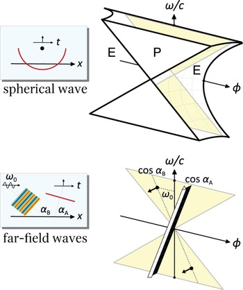
It is also interesting to analyze what happens when the source is in the far field – illustrated in the lower half of Fig. 2. In the example, there are two far-field sources – one generating a sinusoidal wave front with frequency ω0; the other generating an impulsive wave front (a Dirac pulse). The sinusoid generates two spectral points in the 2D spectrum, point-symmetric, and positioned along an imaginary diagonal line of slope cos αA/c and aligned with ω = ±ω0 (see Box III.1 for details). In other words, the sinusoidal wave front is composed of two plane waves with opposing frequencies. The diagonal line's slope changes within the shaded triangular region as a function of the angle of arrival αA of the wave front. The second wave front generates a Dirac function spanning the entire diagonal line with slope cos αB/c, which also changes as a function of αB. This means that a Dirac source in the far-field excites all the frequencies in the 2D spectrum associated with its direction of propagation.
Definition of the spatiotemporal Fourier transform
If the x-axis, for instance, represents the microphone array, the continuous Fourier transform of the wave field is defined by
 $$P\lpar \phi\comma \; \omega\rpar = \vint_{\open R}\vint_{\open R}p\lpar x\comma \; t\rpar e^{-j\lpar \phi x + \omega t\rpar } dtdx\comma \;$$
where ϕ is the spatial frequency in rad/m (also known as wavenumber) and ω is the temporal frequency in rad/s. The inverse transform is given by
 $$p\lpar x\comma \; t\rpar = \displaystyle{1 \over 4\pi^2} \vint_{\open R} \vint_{\open R}P\lpar \phi\comma \; \omega\rpar e^{j\lpar \phi x + \omega t\rpar }d\omega d \phi.$$
The first relevant aspect of (10) is that the Fourier transform of a wave field is an orthogonal expansion into plane wave components. Each plane wave is characterized by a spatiotemporal frequency pair (ϕ0, ω0), which determines the respective frequency of oscillation and direction of propagation. For every frequency pair, we get
 $$P\lpar \phi\comma \; \omega\rpar = 2\pi \delta \left(\omega - \omega_0 \right)2\pi \delta \left(\phi - \phi_{0} \right)\comma \;$$
which can alternatively be expressed as
 $$P\lpar \phi\comma \; \omega\rpar = 2\pi \delta \left(\omega - \omega_{0} \right)2\pi \delta \left(\phi - \cos \alpha_0 \displaystyle{\omega_0 \over c} \right)\comma \;$$
where α0 is the propagation angle with respect to the x-axis. For a general source in the far field, we get
 $$P\lpar \phi\comma \; \omega\rpar = S\lpar \omega\rpar 2\pi \delta \left(\phi - \cos \alpha \displaystyle{\omega \over c} \right).$$
The Dirac function $\delta \left(\phi - \cos \alpha \displaystyle{\omega \over c} \right)$
is non-zero for
$\delta \left(\phi - \cos \alpha \displaystyle{\omega \over c} \right)$
is non-zero for $\phi = \cos \alpha \displaystyle{\omega \over c}$
, and is weighted by the Fourier transform of the source signal. The orientation of the Dirac function is given by the line crossing the ϕω-plane with slope
$\phi = \cos \alpha \displaystyle{\omega \over c}$
, and is weighted by the Fourier transform of the source signal. The orientation of the Dirac function is given by the line crossing the ϕω-plane with slope $\displaystyle{\partial\phi \over \partial\omega} = \displaystyle{\cos \alpha \over c}$
, which depends only on the speed and direction of propagation of the wave front.
$\displaystyle{\partial\phi \over \partial\omega} = \displaystyle{\cos \alpha \over c}$
, which depends only on the speed and direction of propagation of the wave front.
Note also that, since α ∈ [0, π], the Dirac function is always within a triangular region defined by $\phi^2 \leq \left(\displaystyle{\omega \over c}\right)^2$
. This gives the spectrum of a wave field a characteristic bow-tie shape, since most of the energy comes from plane waves (as opposed to evanescent waves) and they all fall into this region. It also gives a good intuition as to why the Nyquist sampling condition in space is given by ϕ
s
≥ 2ω
m
/c, since this condition prevents spectral images along the ϕ-axis from overlapping and causing spatial aliasing [Reference Ajdler, Sbaiz and Vetterli15].
$\phi^2 \leq \left(\displaystyle{\omega \over c}\right)^2$
. This gives the spectrum of a wave field a characteristic bow-tie shape, since most of the energy comes from plane waves (as opposed to evanescent waves) and they all fall into this region. It also gives a good intuition as to why the Nyquist sampling condition in space is given by ϕ
s
≥ 2ω
m
/c, since this condition prevents spectral images along the ϕ-axis from overlapping and causing spatial aliasing [Reference Ajdler, Sbaiz and Vetterli15].
Green's function
Consider a point source with source signal s(t) = δ(t) located at r = r p , such that
 $$p\lpar {\bf r}\comma \; t\rpar = \displaystyle{\delta\left(t - \displaystyle{\left\Vert {\bf r}-{\bf r}_{p}\right\Vert \over c} \right)\over 4\pi \left\Vert {\bf r} - {\bf r}_{p}\right\Vert}.$$
Plugging p(x, t) into (10) yields [Reference Ajdler, Sbaiz and Vetterli15]
 $$P\lpar \phi\comma \; \omega\rpar = \displaystyle{1 \over 4j} H_{0}^{\lpar 1\rpar \ast} \left(\sqrt{y_{p}^{2} + z_{p}^{2}} \sqrt{\left(\displaystyle{\omega \over c} \right)^{2} - \phi^2}\right)e^{-j\phi x_{p}}.$$
where H 0 (1)* is the zeroth-order Hankel function of the first kind.
Evanescent waves belong to the part of the 2D spectrum where | ϕ | > | ω |/c. Note that for | ϕ | > | ω |/c, the argument of the Hankel function in (15) becomes imaginary, and (15) can be rewritten as [Reference Ajdler, Sbaiz and Vetterli15]
 $$P\lpar \phi\comma \; \omega\rpar = \displaystyle{1 \over 2\pi} K_{0}\left(\sqrt{y_{p}^{2}+z_{p}^{2}} \sqrt{\left(\displaystyle{\omega \over c}\right)^{2} - \phi^2}\right)e^{-j\phi x_{p}}\comma \;$$
where K 0 is the modified Bessel function of the second kind and order zero. The asymptotic behavior of K 0 is given by [Reference Williams12]
 $$K_0 \lpar x\rpar \sim \sqrt{\displaystyle{\pi \over 2x}} e^{-x}\comma \; \quad x \gt 0.$$
Thus, the evanescent energy decays exponentially along the spatial frequency beyond | ϕ | = | ω |/c.
In general, it can be shown that wave fields are composed of propagating plane waves traveling in different directions with different frequencies, plus the (mostly residual) evanescent components [Reference Pinto and Vetterli17]. This is analogous to 1D signals being composed of complex exponentials with different frequencies. The spectrum of plane waves and evanescent energy is obtained through the spatiotemporal Fourier transform.
IV. SAMPLING IN SPACE AND TIME
We have seen that acoustic signals are approximately band-limited in a special, non-separable way, defined by the spectral support of the Green's function in free field. In the context of signal processing, this leads to important sampling and interpolation results.
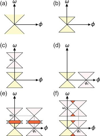
In traditional signal processing, a system is composed of three stages: sampling, processing, and interpolation. The system takes as input a continuous-time signal, and generates a discrete version by taking periodic samples with a given sampling frequency ω s . If the signal is band-limited with maximum frequency ω m and the sampling frequency satisfies the Nyquist condition, given by ω s ≥ 2ω m , then the samples contain all the information needed to reconstruct the original continuous-time signal, which can be done with an interpolation filter. In many scenarios in acoustic signal processing, one deals with sources that are sufficiently far away from the region of interest. As a consequence, temporally band-limited sources give rise to spatially and temporally band-limited wave fields. This also implies that the sound pressure can be sampled at discrete locations in space without a significant loss of information, as long as the Nyquist sampling condition is satisfied [Reference Ajdler, Sbaiz and Vetterli15]. To satisfy the Nyquist condition in space, the spatial sampling frequency ϕs must be chosen such that ϕ s ≥ 2ω m /c. The spatial samples can then be used to resynthesize the “analog” wave front, as predicted by the Huygens principle. Once in discrete space and time, the tools and algorithms of 2D DSP can be used to process the wave field. The effects of sampling in space and time are illustrated in Fig. 3.
Effects of sampling in space and time: (a) non-band-limited spectrum; (b) band-limited spectrum; (c) (aliasing-free) temporal sampling; (d) (aliasing-free) spatial sampling; (e) temporal aliasing; (f) spatial aliasing.
V. SPACE–TIME–FREQUENCY ANALYSIS
One of the limitations of the Fourier transform in the analysis of wave fields is that it is non-local. Similarly to the time-domain signals whose frequency content is time dependent, the plane-wave content of wave fields is space dependent. As a consequence, the Fourier transform in its standard form has no spatial resolution. To visualize this limitation, take for example a point source in space radiating a spherical wave front. The curvature of the wave front is not the same everywhere; it is much more pronounced in the vicinity of the source, and more flat as we move farther (eventually converging to a far-field wave front). This suggests that the plane wave content of the wave field tends to vary considerably, depending on the region in space where the wave field is observed. Thus, the Fourier analysis of the wave field requires some form of spatial resolution.
One way of addressing this problem is to represent the wave field in a space–frequency domain, where the spatial resolution can be increased to the detriment of spatial frequency resolution. In practice, this means applying a spatial window along the microphone array, and selecting a window function and respective length such that it provides the desired balance between space and frequency resolution. If the input wave field is a plane wave, the spectral line that represents its frequency and direction of propagation “opens up” into a smooth support function centered at the same point. This implies that, by limiting the size of the analysis window, the plane waves become less concentrated in small regions of the spectrum, affecting the overall sparsity of the spatiotemporal Fourier transform. The result of the spatial windowing operation is illustrated in the upper half of Fig. 4.
Windowed Fourier transform of a Dirac source in the far-field (top) and the near-field (bottom). The triangular pattern opens as the source gets closer to the microphone array, closes as the source gets farther away, and skews left and right according to the minimum and maximum angles of incidence of the wave front. The ripples on the outside of the triangle are caused by the sinc-function effect of spatial windowing, and are directed toward the average direction of incidence of the wave front.
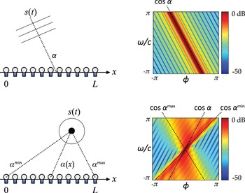
Another important limitation of the Fourier transform comes from its implicit assumption of infinitely long spatial axis, making the sources always appear in the near field (in the analytical sense). Thus, it provides little basis for the practical case: a microphone array with finite length. The space–frequency analysis, on the contrary, provides such a mathematical basis. The result is an “intermediate-field” spectral shape that varies between a fully open triangular shape (near-field) and an infinitely compact Dirac line (far-field). The aperture of the triangle is directly affected by the local curvature of the wave front. This is illustrated in the lower half of Fig. 4.
VI. PROCESSING WAVE FIELDS IN DISCRETE SPACE AND TIME
The work carried out by Dennis Gabor in 1946 on the time–frequency representation of non-stationary signals [Reference Gabor18] had an impact in the area of Fourier analysis well beyond that of the development of the short-time Fourier transform. The work essentially led to a generalized view of orthogonal transforms, based on the concept that different types of signals require different partitioning of the time–frequency plane. Music signals, for instance, are better represented by a uniform partitioning of the spectrum, due to their harmonic nature. Electrocardiographic signals, on the contrary, are mostly characterized by low-frequency components generated by the heart beat plus the wide band noise generated by the surrounding muscles. For this type of signals, a dyadic partitioning of the spectrum – with higher resolution for lower frequencies – is a more appropriate representation. Such representations can be obtained through a class of discrete-time structures known as filter banks, which consist of a sequence of filters and rate converters organized in a tree structure (see, e.g., Vaidyanathan [Reference Vaidyanathan19] and Vetterli et al. [Reference Vetterli and Kovacevic20, Reference Vetterli, Kovacevic and Goyal21]).
Filter banks are a powerful tool used for modeling systems and obtaining efficient representations of a given class of signals through linear transforms that are invertible and critically sampled, and, in many cases, computationally efficient. In particular, filter banks can be used to implement the discrete version of orthogonal transforms, such as the Fourier transform. For example, the frequency coefficients provided by the discrete Fourier transform (DFT) can be interpreted as the output of a uniform filter bank with as many bandpass filters as the number of coefficients. If the signal being transformed is multidimensional – say, a spatio-temporal signal – then the theory of multidimensional filter banks can be used instead, resulting in the typical filter bank structure shown in Fig. 5.
Typical structure of a multidimensional filter bank. (a) The filter bank structure is similar to the 1D case, except that the filters and rate converters are multidimensional. The z-transform vector is defined such that, in the 2D spatiotemporal domain, z = (z
x
,z
t
), and N is a diagonal resampling matrix given by ${\bf N} = \left[\matrix{N_x & 0 \cr 0 & N_t} \right]$
. The number of filters is determined by the size of the space of coset vectors
${\bf N} = \left[\matrix{N_x & 0 \cr 0 & N_t} \right]$
. The number of filters is determined by the size of the space of coset vectors ${\open K}^{2} \subset {\open Z}^{2}$
(assuming m = 2 from the figure), which is essentially the space of all combinations of integer vectors
${\open K}^{2} \subset {\open Z}^{2}$
(assuming m = 2 from the figure), which is essentially the space of all combinations of integer vectors ${\bf k} = \left[\matrix{k_{x}\cr k_{t}} \right]$
from
${\bf k} = \left[\matrix{k_{x}\cr k_{t}} \right]$
from ${\bf k} = \left[\matrix{0 \cr 0} \right]$
to
${\bf k} = \left[\matrix{0 \cr 0} \right]$
to ${\bf k} = \left[\matrix{N_{x}-1\cr N_{t}-1}\right]$
. (b) The equivalent polyphase representation is characterized by a delay chain composed of vector delay factors z
−k
= z
x
−k
x
z
t
−k
t
and the resampling matrix N, which generate 2D sample blocks of size N
x
× N
t
from the input signal and vice versa. If the filter bank is separable, the filtering operations can be expressed as a product between transform matrices associated with each dimension.
${\bf k} = \left[\matrix{N_{x}-1\cr N_{t}-1}\right]$
. (b) The equivalent polyphase representation is characterized by a delay chain composed of vector delay factors z
−k
= z
x
−k
x
z
t
−k
t
and the resampling matrix N, which generate 2D sample blocks of size N
x
× N
t
from the input signal and vice versa. If the filter bank is separable, the filtering operations can be expressed as a product between transform matrices associated with each dimension.
The generalization of filter banks theory (see, e.g., [Reference Vaidyanathan19]) consists of using multidimensional filters to obtain the different frequency bands from the input spectrum and using sampling lattices to regulate the spectral shaping prior to and after the filtering operations. Similarly to the 1D case, the synthesis stage of the filter bank can be designed such that the output signal is a perfect reconstruction of the input.
A) Realization of spatiotemporal orthogonal transforms
Spatiotemporal orthogonal transforms can be obtained through any combination of orthogonal bases applied separately to the spatial and temporal dimensions of the discretized sound field. Examples of transforms that can be used to exploit the temporal evolution of the sound field include the DFT, the discrete cosine transform (DCT), and the discrete wavelet transform (DWT). The DFT and the DCT are better suited for audio and speech sources, due to their harmonic nature, whereas the DWT can be better suited for impulsive and transient-like sources. In the spatial domain, the choice of basis takes into account different factors, such as the position of the sources and the geometry of the acoustic environment – which influence the diffuseness of sound and the curvature of the wave field – as well as the geometry of the observation region (for instance, if it is not a straight line). The Fourier transform, as we have shown, provides an efficient representation of the wave field on a straight line.
The definition of the discrete spatiotemporal Fourier transform is explained in more detail in Box VI.1, and two examples are illustrated in Figs 6(c) and 7(c).
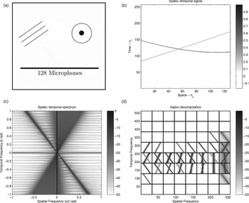
Far-field and intermediate-field sources driven by a Dirac pulse, observed on a linear microphone array. (a) Acoustic scene; (b) spatiotemporal signal p[n]; (c) spatiotemporal DFT P[b]; (d) short spatiotemporal Fourier transform P i[b].
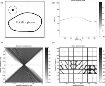
Intermediate-field source driven by a Dirac pulse and observed on a curved microphone array. (a) Acoustic scene; (b) spatiotemporal signal p[n]; (c) spatiotemporal DFT P[b]; (d) short spatiotemporal Fourier transform P i[b].
Definition of the windowed Fourier transform
The way of implementing a spatiotemporal Fourier transform with spatial resolution is by defining P(x 0,ϕ,ω) such that
 $$P\lpar x_{0}\comma \; \phi\comma \; \omega\rpar =\vint_{0}^{L}\vint_{\open R}p\lpar x\comma \; t\rpar w\lpar x-x_{0}\rpar \, e^{-j\lpar \phi x+\omega t\rpar }dtdx\comma \;$$
where w(x − x 0) is a spatial window function of length L. For a source in the far field, the “short-space” Fourier transform replaces the Dirac spectral support by the Fourier transform of the window function, W(ω). The result in (14) then becomes
 $$P\lpar x_{0}\comma \; \phi\comma \; \omega\rpar = S \lpar \omega\rpar W \left(\phi - \cos \alpha \displaystyle{\omega \over c} \right)\, e^{-j\phi x_{0}}.$$
Similarly to what happens in time–frequency analysis, the limited length of the spatial window introduces uncertainty in the frequency domain, by spreading the support function across ϕ. In practice, this means that two wave fronts that propagate with a similar angle may not be resolved in the frequency domain, due to the overlapping of their respective support functions. This uncertainty reflects the trade-off between spatial resolution and spatial frequency resolution.
In addition, the use of windowing in space makes it easier to estimate the Fourier transform of a curved wave front (which is the general case). A good approximation is given by
 $$\eqalign{& P\lpar x_{0}\comma \; \phi\comma \; \omega\rpar \cr &\quad = \left\{\matrix{S\lpar \omega\rpar W\lpar 0\rpar e^{-j\phi x_{0}}\comma \; \hfill &\lpar \phi\comma \; \omega\rpar \in {\cal C}\comma \; \hfill \cr S\lpar \omega\rpar W\left(\phi - \cos \tilde{\alpha} \displaystyle{\omega \over c}\right)e^{-j\phi x_{0}}\comma \; \hfill &\lpar \phi\comma \; \omega\rpar \notin {\cal C}\comma \; \hfill}\right.}$$
where ${\cal C}$
is a point-symmetric region where, for ω ≥ 0,
${\cal C}$
is a point-symmetric region where, for ω ≥ 0, ${\cal C}=\left\{\lpar \phi\comma \; \omega\rpar \colon \phi_{min} \leq \phi \leq \phi_{max} \right\}$
, given
${\cal C}=\left\{\lpar \phi\comma \; \omega\rpar \colon \phi_{min} \leq \phi \leq \phi_{max} \right\}$
, given $\cos \tilde{\alpha} = \displaystyle{1 \over L}\vint_{0}^{L}\cos \alpha \lpar x\rpar dx$
,
$\cos \tilde{\alpha} = \displaystyle{1 \over L}\vint_{0}^{L}\cos \alpha \lpar x\rpar dx$
, $\phi_{min} = \cos \alpha_{max} \displaystyle{\omega \over c}$
, and
$\phi_{min} = \cos \alpha_{max} \displaystyle{\omega \over c}$
, and $\phi_{max} =\cos \alpha_{min}\displaystyle{\omega \over c}$
. What the result in (20) says is that, as the analysis window gets closer to the source, the main lobe of the support function spreads along the region
$\phi_{max} =\cos \alpha_{min}\displaystyle{\omega \over c}$
. What the result in (20) says is that, as the analysis window gets closer to the source, the main lobe of the support function spreads along the region ${\cal C}$
, which is defined by the minimum and maximum angles of incidence of the wave front with the x-axis, α
min
and α
max
. The intuition behind this is that a curved wave front is a superposition of far-field wave fronts with different propagation angles (note that (19) is obtained from (20) when α
min
= α
max
).
${\cal C}$
, which is defined by the minimum and maximum angles of incidence of the wave front with the x-axis, α
min
and α
max
. The intuition behind this is that a curved wave front is a superposition of far-field wave fronts with different propagation angles (note that (19) is obtained from (20) when α
min
= α
max
).
Definition of discrete spatiotemporal transforms
The general formulation of a 2D spatiotemporal orthogonal transform is given by
 $$P\lsqb {\bf b}\rsqb = \sum_{{\bf n} \in {\open Z}^{2}}p\lsqb {\bf n}\rsqb \upsilon_{b_{x}\comma n_{x}}^{\ast}\psi_{b_{t}\comma n_{t}}^{\ast}\comma \; \, {\bf b} \in {\open Z}^{2}$$
and
 $$p\lsqb {\bf n}\rsqb = \sum_{{\bf b} \in {\open Z}^{2}} P \lsqb {\bf b}\rsqb \upsilon_{b_{x}\comma n_{x}} \psi_{b_{t}\comma n_{t}}\comma \; \, {\bf n}\in {\open Z}^{2}\comma \;$$
where n = [n x , n t ] are the discrete spatiotemporal indexes, b = [b x , b t ] are the transform indexes, p[n] is the discrete spatiotemporal signal, and P[b] are the spatiotemporal transform coefficients. The bases represented by υ b x ,n x and ψ b t ,n t are spatial and temporal orthogonal bases, respectively.
In matrix notation, (21) and (22) can be written as
 $${\bf Y} = {\bf \Upsilon}{\bf P}{\bf \Psi}^{H}$$
and
 $${\bf P} = {\bf \Upsilon}^{H}{\bf Y}{\bf \Psi}\comma \;$$
where P, Y, ϒ, and Ψ are the matrix expansions of p[n], P[b], υ b x ,n x and ψ b t ,n t , respectively.
The results in (23) and (24) show that a spatiotemporal orthogonal transform is simply a matrix product between the input samples and the transformation matrices ϒ and Ψ. The transform can thus be expressed as a multidimensional filter bank structure similar to the one shown in Fig. 5, where the block ∏ m H m represents a left product by ϒ and a right product by Ψ H , and ∏ m F m represents a left product by ϒ H and a right product by Ψ. The input signal p[n] of size N x × N t is decomposed by the analysis stage of the filter bank into a transform matrix P[b] of equal size, and reconstructed back to p[n] by the synthesis stage.
To perform a spatiotemporal DFT, the basis functions are defined as
 $$\upsilon_{b_{x}\comma n_{x}} = \displaystyle{1 \over \sqrt{N_x}} e^{j\displaystyle{2\pi \over N_{x}} b_x n_x}\, {\rm and}\, \psi_{b_{t}\comma n_{t}} = \displaystyle{1 \over \sqrt{N_t}} e^{j\displaystyle{2\pi \over N_t} b_t n_t}\comma \;$$
where b x = 0, …, N x − 1, n x = 0, …, N x − 1, b t = 0, …, N t − 1, and n t = 0, …, N t − 1. This implies that ϒ and Ψ are DFT matrices of size N x × N x and N t × N t respectively.
B) Realization of lapped orthogonal transforms (LOTs)
A LOT is a class of linear transforms where the input signal is split up into smaller overlapped blocks before each block is projected onto a given basis (and typically processed individually). A perfect reconstruction of the input signal is obtained by inverting the individual blocks and adding them through a technique known as overlap-and-add [Reference Malvar22]. A spatiotemporal LOT is the kind of transform that is needed to perform the type of analysis described in Section V.
The multidimensional filter bank structure of Fig. 5 can be converted into a lapped transform simply by applying the resampling matrix ${\bf N}\bond {\bf O}$
instead of N, where
${\bf N}\bond {\bf O}$
instead of N, where ${\bf O} = \left[\matrix{O_{x} & 0\cr 0 & O_{t}} \right]$
contains the number of overlapping samples O
x
and O
t
in each dimension. Without loss of generality, we assume that
${\bf O} = \left[\matrix{O_{x} & 0\cr 0 & O_{t}} \right]$
contains the number of overlapping samples O
x
and O
t
in each dimension. Without loss of generality, we assume that ${\bf O} = \displaystyle{1 \over 2} {\bf N}$
, representing 50% of overlapping in both dimensions. Note, however, that since the resulting number of samples is greater than the number of samples of the input signal, the filter bank generates an oversampled transform. This problem can be solved with the use of special subsampled bases, such as the MDCT basis [Reference Malvar22].
${\bf O} = \displaystyle{1 \over 2} {\bf N}$
, representing 50% of overlapping in both dimensions. Note, however, that since the resulting number of samples is greater than the number of samples of the input signal, the filter bank generates an oversampled transform. This problem can be solved with the use of special subsampled bases, such as the MDCT basis [Reference Malvar22].
Through the use of LOTs, a spatiotemporal version of the short-time Fourier transform can then be defined, by applying the method shown in Box VI.2. Examples of the short spatiotemporal Fourier transform of a sound field are illustrated in Figs 6(d) and 7(d).
Definition of discrete Lapped spatiotemporal transforms
The decomposition of p[n] into overlapped blocks p i [n] can be written as
 $$p_{\bf i} \lsqb {\bf n}\rsqb = p\lsqb {\bf n}\rsqb \comma \; \, {\bf n} = \displaystyle{{\bf N} \over 2} {\bf i}\comma \; \ldots\comma \; \displaystyle{{\bf N} \over 2} \lpar {\bf i} + {\bf 2}\rpar - {\bf 1}\comma \; \, {\bf i}\in {\open I}^{2}\comma \;$$
where ${\bf i} = \left[\matrix{i_x \cr i_t} \right]$
is the block index and
${\bf i} = \left[\matrix{i_x \cr i_t} \right]$
is the block index and ${\open I}^{2}\subset {\open Z}^{2}$
is the respective set of block indexes. The notation
${\open I}^{2}\subset {\open Z}^{2}$
is the respective set of block indexes. The notation ${\bf n} = \displaystyle{{\bf N} \over 2} {\bf i}\comma \; \ldots\comma \; \displaystyle{{\bf N} \over 2} \lpar {\bf i} + {\bf 2}\rpar - {\bf 1}$
means that
${\bf n} = \displaystyle{{\bf N} \over 2} {\bf i}\comma \; \ldots\comma \; \displaystyle{{\bf N} \over 2} \lpar {\bf i} + {\bf 2}\rpar - {\bf 1}$
means that $n_{x} = \displaystyle{N_{x} \over 2} i_{x}\comma \; \ldots\comma \; \displaystyle{N_{x} \over 2} \lpar i_{x} + 2\rpar - 1$
and
$n_{x} = \displaystyle{N_{x} \over 2} i_{x}\comma \; \ldots\comma \; \displaystyle{N_{x} \over 2} \lpar i_{x} + 2\rpar - 1$
and $n_{t} = \displaystyle{N_{t} \over 2} i_{t}\comma \; \ldots\comma \; \displaystyle{N_t \over 2} \lpar i_{t} + 2\rpar - 1$
. The vector integers are defined as
$n_{t} = \displaystyle{N_{t} \over 2} i_{t}\comma \; \ldots\comma \; \displaystyle{N_t \over 2} \lpar i_{t} + 2\rpar - 1$
. The vector integers are defined as ${\bf 0} = \left[\matrix{0 \cr 0} \right]$
,
${\bf 0} = \left[\matrix{0 \cr 0} \right]$
, ${\bf 1} = \left[\matrix{1 \cr 1} \right]$
, and so on. Note also that, in order to handle the blocks that go outside the boundaries of n, we consider the signal to be circular (or periodic) in both dimensions. This presents an advantage over zero-padding, in particular, when the spatial “axis” is closed.
${\bf 1} = \left[\matrix{1 \cr 1} \right]$
, and so on. Note also that, in order to handle the blocks that go outside the boundaries of n, we consider the signal to be circular (or periodic) in both dimensions. This presents an advantage over zero-padding, in particular, when the spatial “axis” is closed.
Denoting ϕ [b, n] = υ b x ,n x ψ b t ,n t , the direct and inverse transforms for each block are given by
 $$P_{\bf i}\lsqb {\bf b}\rsqb = \sum_{{\bf n}={\bf 0}}^{{\bf N}{\bf 1} - {\bf 1}} p_{\bf i} \lsqb {\bf n}\rsqb \varphi^{\ast} \lsqb {\bf b}\comma \; {\bf n}\rsqb \comma \; \, {\bf b} = {\bf 0}\comma \; \ldots\comma \; {\bf N}{\bf 1} - {\bf 1}$$
and
 $$\hat{p}_{\bf i}\lsqb {\bf n}\rsqb = \sum_{{\bf b} = {\bf 0}}^{{\bf N}{\bf 1} - {\bf 1}}P_{\bf i}\lsqb {\bf b}\rsqb \varphi\lsqb {\bf b}\comma \; {\bf n}\rsqb \comma \; \, {\bf n} = {\bf 0}\comma \; \ldots\comma \; {\bf N}{\bf 1} - {\bf 1}.$$
Finally, the reconstruction of p[n] through overlap-and-add is given by
 $$p\lsqb {\bf n}\rsqb = \sum_{{\bf i}\in {\open I}^{2}} \hat{p}_{\bf i} \left[{\bf n} - \displaystyle{1 \over 2}{\bf N}{\bf i}\right]\comma \; \, {\bf n}\in {\open Z}^{2}.$$
C) Spatiotemporal filter design
In DSP, filtering is the cornerstone operation when it comes to manipulating signals, images, and other types of data. It is arguably the most used DSP technique in modern technology and electronic devices, as well as in the domain of Fourier analysis in general. The outstanding variety of applications of filtering go beyond the simple elimination of undesired frequencies in signals: it allows, for example, the elimination of several types of interferences, the cancellation of echoes in two-way communications, and the frequency multiplexing of radio signals. Moreover, the theory led to the invention of filter banks, and hence the development of new types of linear transforms and signal representations.
In array signal processing (see, e.g., Johnson et al. [Reference Johnson and Dudgeon23]), there exists a similar concept called spatial filtering (or beamforming). A spatial filter is a filter that favors a given range of directions in space, implemented directly through the array of sensors. The sensors are synchronized such that there is phase alignment for a desired angle of arrival and phase opposition for the other angles. Spatial filters have been used in many contexts throughout history with enormous success – most notably during warfare with the use of radars, and during the era of wireless communications with the use of antennas. Other applications include sonar, seismic wave monitoring, spatial audio, noise cancellation, and hearing aids technology. As long as more than one sensor is available, it is always possible to implement a spatial filter. The human auditory system, for example, uses an array of two sensors (the ears) to localize the sound sources in space.
Similarly to time-domain signals, representing sound fields in the spatiotemporal Fourier domain enables the design of filters in a much more intuitive fashion. One of the greatest attributes of the Fourier transform is that it allows the interpretation of convolutional filtering in terms of intuitive parameters such as the cut-off frequencies, stop-band attenuation, and phase response. For instance, a filter can be sketched in the Fourier domain such that it has a unitary response for a given range of frequencies (pass-band) and a high attenuation for the remaining frequencies (stop-bands), plus an equiripple magnitude response and a linear phase. Using existing algorithms [Reference Oppenheim and Schafer24], the ideal filter can be translated into a realizable filter that optimally obtains the desired response.
In spatiotemporal Fourier analysis, the same reasoning can be used: we can sketch a spatial filter in the Fourier domain such that it has a unitary response for every plane wave within a given range of directions (pass-band) and a high attenuation for the remaining plane waves (stop-bands), plus any additional magnitude and phase constraints. The ideal filter can be translated into a realizable filter by using two-dimensional filter design techniques. Once the spatiotemporal filter coefficients are obtained, the filtering operation can be performed either in the spatiotemporal domain, using the convolution formula, or in the Fourier domain, using the convolution property of the Fourier transform. This process is described in Box VI.3.
Spatiotemporal filtering
A spatiotemporal filter is a 2D discrete sequence defined as h[n] = h[n x ,n t ] with DFT coefficients h[b] = H[b x ,b t ]. If the input signal is p[n], then that spatiotemporal filtering operation is given by a 2D circular convolution [Reference Oppenheim and Schafer24],
 $$y\lsqb {\bf n}\rsqb = \sum_{\rho = 0}^{N_{x} - 1}\sum_{\tau = 0}^{N_{t} - 1} p \lsqb \rho\comma \; \tau\rsqb h\lsqb \lpar \lpar n_{x} - \rho\rpar \rpar _{N_{x}}\comma \; \lpar \lpar n_{t} - \tau\rpar \rpar _{N_{t}}\rsqb \comma \;$$
where ((·)) N = · mod N. Unlike beamforming, the output of (30) is the 2D signal y[n] representing the entire wave field (i.e., with spatial information).
Using the convolution property of the DFT, it follows that
 $$Y\lsqb {\bf b}\rsqb = P\lsqb {\bf b}\rsqb H\lsqb {\bf b}\rsqb .$$
To specify the parameters of the ideal filter, we first need to decide what is the purpose of the filter. A reasonable goal is to focus on the wave fronts originating from a particular point in space – perhaps the location of a target source – while suppressing every other wave front with a different origin. For this purpose, the expression of the spatiotemporal spectrum of an intermediate-field source can be used to specify the parameters of the ideal filter.
Recall the results from Box V.1. According to (20), the maximum concentration of energy is contained within the region defined by the triangular support (i.e., for $\lpar \phi\comma \; \omega\rpar \in {\cal C}$
). Thus, the ideal filter can be defined in discrete space and time as
$\lpar \phi\comma \; \omega\rpar \in {\cal C}$
). Thus, the ideal filter can be defined in discrete space and time as
 $$H\lsqb {\bf b}\rsqb = \left\{\matrix{ 1 &\comma \; {\bf b}\in {\cal C}\comma \; \cr 0 & \comma \; \, {\bf b}\notin {\cal C}\comma \; } \right.$$
where ${\cal C} = \left\{{\bf b}\colon b_{x}^{min}\leq b_{x}\leq b_{x}^{max} \comma \; \, b_{t} \geq <xref ref-type="disp-formula" rid="eqn0">0</xref> \right\}$
, and point-symmetric for b
t
< 0. The parameters b
x
min
and b
x
max
are the discrete counterparts of ϕ
min
and ϕ
max
, and are given by
${\cal C} = \left\{{\bf b}\colon b_{x}^{min}\leq b_{x}\leq b_{x}^{max} \comma \; \, b_{t} \geq <xref ref-type="disp-formula" rid="eqn0">0</xref> \right\}$
, and point-symmetric for b
t
< 0. The parameters b
x
min
and b
x
max
are the discrete counterparts of ϕ
min
and ϕ
max
, and are given by $b_{x}^{min} = \cos \alpha^{max} \displaystyle{b_t \over c} \left(\displaystyle{T_x N_x \over N_t} \right)$
and
$b_{x}^{min} = \cos \alpha^{max} \displaystyle{b_t \over c} \left(\displaystyle{T_x N_x \over N_t} \right)$
and $b_{x}^{max} = \cos \alpha^{min} \displaystyle{b_t \over c} \left(\displaystyle{T_x N_x \over N_t} \right)$
, where T
x
is the sampling period in space. The relation between the focus point and the filter specifications is illustrated in Fig. 12.
$b_{x}^{max} = \cos \alpha^{min} \displaystyle{b_t \over c} \left(\displaystyle{T_x N_x \over N_t} \right)$
, where T
x
is the sampling period in space. The relation between the focus point and the filter specifications is illustrated in Fig. 12.
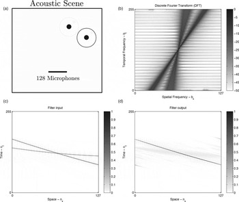
Figures 8–11 show various examples of how this type of non-separable spatio-temporal filtering can be used to suppress point sources in space (in the near-field and far-field) without the loss of spatial information of the remaining sources in the output signal. In these examples, the ideal filter is designed using the method of (32), with cutoff angles given by αStop max = 1.05α max , α Pass max = 0.95α max , α Pass min = 1.05α min , and α Stop min = 0.95α min , where α min and α max are the minimum and maximum incidence angles of the wave front we wish to filter (see Fig. 12). The ideal filter H[b] is then applied directly to the input sound field spectrum P[b] using (31), without actually going through a 2D filter design algorithm. Obviously, applying an ideal filter with flat pass- and stop-bands is not advised in practical implementations; we do it here only as a proof-of-concept.
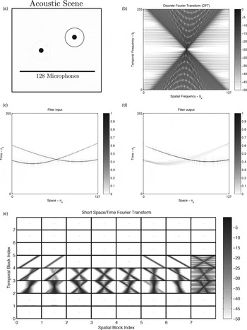
Example of filtering directly in the spatiotemporal Fourier domain (with no lapped transform). (a) The acoustic scene consists of two Dirac sources in the intermediate-field. The goal is to suppress the dashed source. (b) DFT along the entire spatial axis. (c) Filter input. (d) Filter output.
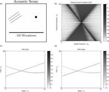
Example of filtering directly in the spatiotemporal Fourier domain (with no lapped transform). (a) The acoustic scene consists of two Dirac sources, where one is in the intermediate-field and the other in the far-field. The goal is to suppress the dashed source. (b) DFT along the entire spatial axis. (c) Filter input. (d) Filter output.
Example of filtering in the short spatiotemporal Fourier domain. (a) The acoustic scene consists of two Dirac sources in the intermediate-field. The goal is to suppress the dashed source. (b) DFT along the entire spatial axis. (c) Filter input. (d) Filter output. (e) Short spatiotemporal Fourier transform.
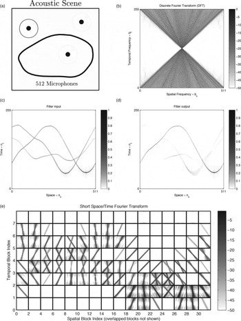
Example of filtering in the short spatiotemporal Fourier domain. (a) The acoustic scene consists of three Dirac sources in the intermediate-field, and a curved microphone array. The goal is to suppress the dashed sources. (b) DFT along the entire spatial axis. (c) Filter input. (d) Filter output. (e) Short spatiotemporal Fourier transform.
Design steps of a spatiotemporal filter. The pass-band region of the filter should enclose the triangular pattern that characterizes the spectrum of a point source.
D) Acoustic wave field coding
Since the early days of DSP, the question of how to represent signals efficiently in a suitable mathematical framework has been paired with the question of how to efficiently store them in a digital medium. The storage of digital audio, in particular, has been marked by two major breakthroughs: (i) the development of pulse-code modulation (PCM) [Reference Oliver and Shannon25], and (ii) the development of perceptual audio coding [Reference Johnston26]. These techniques were popularized, respectively, by their use in Compact Disc technology and MP3 compression; both had a deep impact on the entire industry of audio storage.
The MP3 coding algorithm, in particular, operates by transforming the PCM signal to a Fourier-based domain through the use of a uniform filter bank, where the amplitude of the frequency coefficients is again quantized. The key breakthrough is that the number of bits used for quantizing each coefficient is variable, and, most importantly, dependent on their perceptual significance. Psychoacoustic studies show that a great portion of the signal is actually redundant on a perceptual level. This is related to the way the inner ear processes mechanical waves: the wave is decomposed into frequencies by the cochlea, where each frequency stimulates a local group of sensory cells. If a given frequency is close to another frequency with higher amplitude, it will not be strong enough to overcome the stimulation caused by the stronger frequency, and therefore will not be perceived. For this reason, the use of perceptual criteria in the quantization process gives an average compression ratio of 1/10 over the use of PCM.
In the spatiotemporal analysis of acoustic wave fields, the question arises of how much relevant information is contained in the wave field, and what is the best way of storing it. When the sound pressure is captured by the multiple microphones to be processed by a computer, there is an implicit amplitude quantization of the pressure values in p[n]. The spatiotemporal signal obtained by a linear array, for instance, is in fact a 2D PCM signal. With modern optical media such as Double Layer DVD (approximately 8.55 GB of storage capacity) or BlueRay, we can store about 24 audio channels with 80 min of raw (uncompressed) PCM data. However, if the goal is to store in the order of 100 channels, it is imperative that the data be compressed as efficiently as possible.
The most relevant work on joint compression of audio channels dates back to the development of perceptual audio coding in the early 1990s. When it was realized that mono PCM audio could be efficiently compressed using filter banks theory and perceptual models, the techniques were immediately extended to stereo PCM audio (see, {e.g.}, Johnston et al. [Reference Johnston and Ferreira27] and Herre et al. [Reference Herre, Brandenburg and Lederer28]), and later to an unlimited number of PCM audio channels (see, e.g., Faller et al. [Reference Faller and Baumgarte29] and Herre et al. [Reference Herre, Faller, Ertel, Hilpert, Hoelzer and Spenger30]). The basic premise of these techniques is that the audio channels are highly correlated and therefore can be jointly encoded with high efficiency, using a parametric approach. The correlation criteria can be both mathematically based – for example, using the theory of dimensionality reduction of data sets [Reference Yang, Hongmei, Kyriakakis and Kuo31]; or perceptually motivated – for example, based on the ability of humans to localize sound sources in space [Reference Blauert32]. However, what all these techniques have in common is that they treat the multichannel audio data (i.e., the acoustic wave field) as multiple functions of time, and not as a function of space and time such as the one the wave equation provides.
So, rather than treating the multichannel audio data as multiple functions of time, we can treat the entire wave field as a single multidimensional function of space and time, and perform the actual coding in the multidimensional Fourier domain [Reference Pinto and Vetterli33]. When the spatiotemporal signal p[n] is transformed into the spatiotemporal Fourier domain, there is an implicit decorrelation of the multichannel audio data. This decorrelation is optimal for harmonic sources in the far-field, as these are the basic elements of the spatio-temporal Fourier transform. As a consequence, by quantizing the transform coefficients in P[b] instead of jointly coding the multichannel signals p[0, n t ], p[1, n t ], …, p[N x − 1, n t ], we are directly coding the elementary components of the wave field, which are the plane wave coefficients. Then, using rate-distortion analysis, we can obtain a function that relates the number of bits needed to encode the sound field for any given distortion. This rate-distortion analysis is described in Box VI.4.
Spatiotemporal spectral quantization
Suppose we want to compress the wave field observed on a straight line with N x spatial points, by encoding the coefficients of P[b] in the transform domain. The first step is to quantize the amplitude of P[b], so that a limited number of bits is needed to encode the amplitudes of each coefficient. One way to quantize P[b] is by defining P Q[b] such that
 $$P_{\rm Q}\lsqb {\bf b}\rsqb = \hbox{sign} \left\{P\lsqb {\bf b}\rsqb \right\}\left\lfloor {\rm SF} \lsqb {\bf b}\rsqb \left\vert P\lsqb {\bf b}\rsqb \right\vert \right\rfloor\comma \;$$
where SF[b] contains the scale factors of each coefficient, and ⌊·⌋ denotes rounding to the closest lower integer. The purpose of the scale factors is to scale the coefficients of P[b] such that the rounding operation yields the desired quantization noise.
Conversely, the noisy reconstruction of P[b] can be obtained as
 $$\hat{P}\lsqb {\bf b}\rsqb = \hbox{sign}\left\{P_{\rm Q}\lsqb {\bf b}\rsqb \right\}\left(\displaystyle{1 \over {\rm SF}\lsqb {\bf b}\rsqb } \left\vert P_{\rm Q}\lsqb {\bf b}\rsqb \right\vert \right).$$
To determine the number of bits required to encode the quantized coefficients, we need to associate the amplitude values to a binary code book – preferably one that achieves the entropy. In this paper, we consider a Huffman code book similar to the one used in the MPEG standard [34], where code words are organized such that less bits are used to describe lower amplitude values.
Defining Huffman A as an operator that maps the amplitude value A to the corresponding set of bits (or code word) in the Huffman code book, the number of bits R[b] required for each coefficient is given by
 $$R\lsqb {\bf b}\rsqb = \left\vert \hbox{Huffman} \left\{P_{\rm Q}\lsqb {\bf b}\rsqb \right\}\right\vert\comma \;$$
where |·| denotes the size of the set of bits in the resulting code word.
Using the MSE between the input signal p[n] and the output signal $\hat{p}\lsqb {\bf n}\rsqb $
as a measure of distortion, the rate-distortion function D(R) is given by the parametric pair
$\hat{p}\lsqb {\bf n}\rsqb $
as a measure of distortion, the rate-distortion function D(R) is given by the parametric pair
 $$\eqalign{R& = \sum_{{\bf n}={\bf 0}}^{{\bf N}{\bf 1}-{\bf 1}}R\lsqb {\bf b}\rsqb \comma \; \cr D & = \displaystyle{1 \over \det{\bf N}} \sum_{{\bf n}={\bf 0}}^{{\bf N}{\bf 1}-{\bf 1}}\left(p\lsqb {\bf n}\rsqb - \hat{p}\lsqb {\bf n}\rsqb \right)^{2}\comma \; }$$
where R and D are functions of SF[b], with 0 ≤ SF[b] < ∞. In the limiting cases, where SF[b] → 0 and SF[b] → ∞ for all b, (36) yields respectively.
 $$\eqalign{\lim_{{\rm SF}\lsqb {\bf b}\rsqb \rightarrow0}R & =0\comma \; \cr \lim_{{\rm SF}\lsqb {\bf b}\rsqb \rightarrow 0} D & =\hbox{var}\left\{p\lsqb {\bf n}\rsqb \right\}}$$
and
 $$\eqalign{\lim_{{\rm SF}\lsqb {\bf b}\rsqb \rightarrow\infty}R & =\infty\comma \; \cr \lim_{{\rm SF}\lsqb {\bf b}\rsqb \rightarrow\infty}D & =0\comma \; }$$
where var {·} denotes the signal variance (or power), and the last equality comes from the limiting case $\lim_{{\rm SF}\lsqb {\bf b}\rsqb \rightarrow \infty}\hat{P}\lsqb {\bf b}\rsqb = P\lsqb {\bf b}\rsqb $
.
$\lim_{{\rm SF}\lsqb {\bf b}\rsqb \rightarrow \infty}\hat{P}\lsqb {\bf b}\rsqb = P\lsqb {\bf b}\rsqb $
.
Figure 13 shows examples of rate-distortion curves that result of encoding the acoustic wave field observed on a straight line, using the short spatiotemporal Fourier transform (the Gabor domain). In these examples, the acoustic scene is composed of white-noise sources, in order to reduce the influence of the temporal behavior of the wave field in the bit rate R. Also, since we are evaluating the influence of the number of spatial points N x in the final number of bits required, the bit rate is expressed in units of “bits per time sample”.
Experimental rate-distortion curves for white-noise sources in the far-field observed on a straight line. On the left, the D(R) curves are shown for one source encoded in the short spatiotemporal Fourier domain (Gabor domain) with no overlapping. The source is fixed at $\alpha = \displaystyle{{\pi}\over{3}}$
and the number of spatial points N
x
is variable. On the right, the D(R) curves are shown for multiple sources encoded in the short spatiotemporal Fourier domain. The number of spatial points is fixed, N
x
= 64, and the sources are placed at random angles. The black circle shown in each plot indicates R = 2.6 bits/time-sample, which is the average rate of state-of-art perceptual coders.
$\alpha = \displaystyle{{\pi}\over{3}}$
and the number of spatial points N
x
is variable. On the right, the D(R) curves are shown for multiple sources encoded in the short spatiotemporal Fourier domain. The number of spatial points is fixed, N
x
= 64, and the sources are placed at random angles. The black circle shown in each plot indicates R = 2.6 bits/time-sample, which is the average rate of state-of-art perceptual coders.
In both cases, we can observe that the increase in the number of spatial points N x does not increase the bit rate proportionally, but it actually converges to an upper-bound. The reason is that, even though doubling N x also duplicates the number of transform coefficients, the support functions are narrowed to half the width (recall equation (19)), and the trade-off tends to balance itself out. Thus, increasing N x past a certain limit does not increase the spectral information, since all it adds are zero values (i.e., amplitude values that are quantized to zero).
It can also be observed that for lower bit-rates – in the order of those used by perceptual audio coders [Reference Bosi and Goldberg35] – the difference between one channel and a large number of channels is low in terms of MSE. For example, in Fig. 13 (left), the number of bits required to encode 256 channels is 11.3 bits/time-sample, as opposed to the 2.6 bits/time-sample required for encoding one channel. To have a fair comparison, we can consider that a practical codec would require about 20% of bit-rate overhead with decoding information [34], and thus increase the average rate to 13.6 bits/time-sample. Still, compared to encoding one channel, the total bit rate required to support the additional 255 channels is only five times higher.
Another interesting result is that, similarly to what happens when N
x
is increased, the increase in the number of sources does not increase the bit rate proportionally; again, it converges to an upper-bound. This is because the bit rate only increases until the entire triangular region of the spectrum (defined in Box III.1 as $\phi^{2}\leq \left(\displaystyle{\omega \over c}\right)^{2}$
) is filled up with information. Once this happens, the spectral support generated by additional sources will simply overlap with the existing ones.
$\phi^{2}\leq \left(\displaystyle{\omega \over c}\right)^{2}$
) is filled up with information. Once this happens, the spectral support generated by additional sources will simply overlap with the existing ones.
E) Sound field reproduction
Here we give brief descriptions of two approaches for reproducing continuous sound fields. The first is based on the spatiotemporal sampling framework described in Section IV, and acoustic multiple input, multiple output (MIMO) channel inversion, described in the following. The second approach, known under the name of WFS [Reference Berkhout6], is based on the Huygens principle described in Section C.
We note that we cannot do justice to a number of other approaches for reproducing sound fields. Some of them are extensions of WFS [Reference Corteel36,Reference Gauthier and Berry37], some are based on multidimensional channel inversion [Reference Ahrens and Spors8], and there are many approaches based on matching spherical harmonic components between the desired and reproduced 3D sound fields [Reference Gerzon4,538–Reference Ward and Abhayapala40].
1. Sound field reproduction through acoustic MIMO channel inversion
We have already seen one implication of effective spatiotemporal band-limitedness of wave fields in Section IV, that a wave field is essentially determined by its time evolution on a sampling grid of points that satisfies the Nyquist condition ϕ s ≥ 2ω m /c. Here we present a way to use this observation in order to reproduce continuous wave fields by discrete-space processing.
Assume for simplicity that two wave fields are fully band-limited, with the same spatiotemporal spectral support shown in Fig. 3(b). Following the argument from Section IV, the two wave fields are uniquely represented by multidimensional signals obtained through sampling on a spatial grid satisfying the Nyquist condition (refer to Fig. 3(d)). Moreover, one can easily extend that argument and show that if two adequately sampled wave fields are equal in the discrete domain, they are equal in the continuous domain – at any point in space and time [Reference Kolundžija, Faller and Vetterli9].
Transposed to the context of sound field reproduction, this observation states that it is sufficient to reproduce a sound field on a grid of points that satisfies the Nyquist condition; the accurate reproduction (or interpolation) in the remainder of the continuous domain is taken care of by Green's function acting as the interpolation kernel [Reference Kolundžija, Faller and Vetterli9].
Imagine that a loudspeaker array ${\cal L} = \lcub l_{1}\comma \; \, l_{2}\comma \; \, \ldots\comma \; \, l_{L}\rcub $
– not necessarily planar or linear – is used for reproducing a sound field in a continuous area, as shown in Fig. 14(a). Let
${\cal L} = \lcub l_{1}\comma \; \, l_{2}\comma \; \, \ldots\comma \; \, l_{L}\rcub $
– not necessarily planar or linear – is used for reproducing a sound field in a continuous area, as shown in Fig. 14(a). Let ${\cal C} = \lcub c_{1}\comma \; \, c_{2}\comma \; \, \ldots\comma \; \, c_{N}\rcub $
be a grid of control points covering the listening domain
${\cal C} = \lcub c_{1}\comma \; \, c_{2}\comma \; \, \ldots\comma \; \, c_{N}\rcub $
be a grid of control points covering the listening domain ${\cal S}$
and satisfying the Nyquist condition which, as stated earlier, is sufficient to describe a continuous sound field. The acoustic channel G
ji
(ω) between loudspeaker i and control point j is determined by Green's function G
ω(
r
l
i
|
r
c
j
, so the system loudspeakers-control points can be described by an acoustic channel matrix
G
(ω) = [G
ij
(ω)]. In a similar way, any reproduced source s defines an array
A
(ω) of acoustics channels to the control points, given by A
i
(ω) = G
ω(
r
|
r
c
i
) and illustrated in Fig. 14(b). Note that in practice A
i
(ω) are usually obtained from a model (e.g., Green's function in the free field), while G
ij
(ω) are either measured or obtained from a model.
${\cal S}$
and satisfying the Nyquist condition which, as stated earlier, is sufficient to describe a continuous sound field. The acoustic channel G
ji
(ω) between loudspeaker i and control point j is determined by Green's function G
ω(
r
l
i
|
r
c
j
, so the system loudspeakers-control points can be described by an acoustic channel matrix
G
(ω) = [G
ij
(ω)]. In a similar way, any reproduced source s defines an array
A
(ω) of acoustics channels to the control points, given by A
i
(ω) = G
ω(
r
|
r
c
i
) and illustrated in Fig. 14(b). Note that in practice A
i
(ω) are usually obtained from a model (e.g., Green's function in the free field), while G
ij
(ω) are either measured or obtained from a model.
Sound field reproduction through MIMO acoustic channel inversion problem overview.
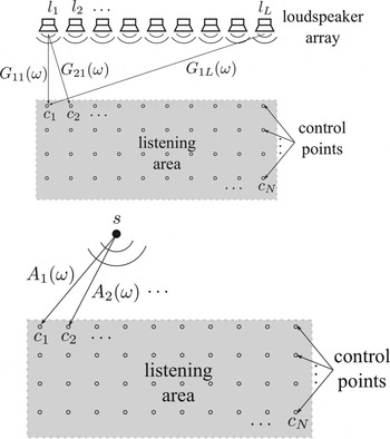
Acoustic MIMO channel inversion
The observation that multi-point reproduction gives a better control over the reproduced sound has been used in active noise control (see [Reference Elliott and Nelson41, Reference Kuo and Morgan42] and references therein) and multichannel room equalization [Reference Miyoshi and Kaneda43]. Multichannel techniques from active noise control later found application in sound field reproduction, either independently [Reference Kirkeby and Nelson44, Reference Kirkeby, Nelson, Orduna-Bustamante and Hamada45] or combined with other approaches, such as WFS [Reference Corteel36, Reference Gauthier and Berry37].
The multi-point sound reproduction through the inversion of an acoustic MIMO channel G (ω) can be expressed in the general form
 $$\matrix{\hbox{minimize}\hfill & \Vert {\bi W}\lpar \omega\rpar \lpar {\bi G}\lpar \omega\rpar {\bi H}\lpar \omega\rpar - {\bi A}\lpar \omega\rpar \rpar \Vert_{x} \hfill \cr \hbox{subject to}\hfill & \hbox{physical constriants}\comma \; \hfill}$$
where
W
(ω) is an error-weighting matrix, x is the chosen weighted-error norm (typically the ${\cal L}^{2}$
-norm), and
H
(ω) is an array of unknown reproduction filters.
${\cal L}^{2}$
-norm), and
H
(ω) is an array of unknown reproduction filters.
The very general term “physical constraints” is usually used to express hard or soft constraints on filters' gains or their frequency-domain variations, but can equally account for geometry-based selection of used loudspeakers [Reference Kolundžija, Faller and Vetterli9, Reference Corteel36, Reference Verheijen46, Reference Spors47]. On the other hand, the weighting matrix W (ω) can assign different importance to errors at different frequencies or different control points, as done in [Reference Kolundžija, Faller and Vetterli9]. One should also note that extending the reproduction to an arbitrary number of sources is done using the principle of superposition, solving (37) for every reproduced sound source separately and combining the outputs into one array of loudspeaker driving signals.
The simplest case of acoustic MIMO channel inversion contains no physical constraints, no error weighting (
W
(ω) =
I
), and minimizes the ${\cal L}^{2}$
-norm of the reproduction error. Its well-known solution obtained through the pseudoinverse of the matrix
G
(ω) is given by
${\cal L}^{2}$
-norm of the reproduction error. Its well-known solution obtained through the pseudoinverse of the matrix
G
(ω) is given by
 $${\bi H}\lpar \omega\rpar = {\bi G}^{+} \lpar \omega\rpar {\bi A} \lpar \omega\rpar .$$
Typically, however, the matrix G (ω) has a very large condition number at low frequencies, and the reproduction filters obtained from (38) are of little practical use. The usual remedy to this problem is the use of a regularized pseudoinverse, computed either through Tikhonov regularizationFootnote 2 [Reference Corteel36, Reference Kirkeby, Nelson, Hamada and Orduna-Bustamante48] or truncated singular value decomposition [Reference Kolundžija, Faller and Vetterli9].
In more general cases, (37) takes a form of a convex program, which can be solved using some readily available solvers, such as [Reference Sturm49] or [Reference Toh, Todd and Tütüncü50].
Figure 15 illustrates the reproduction of sound fields with Sound Field Reconstruction, which is an approach based on the previously described discretization strategy and acoustic MIMO channel inversion [Reference Kolundžija, Faller and Vetterli9].
An illustration of sound field reproduction with an array of loudspeakers, the listening area being to the right (in front) of the loudspeaker array. Figures on the left show snapshot of desired sound fields, while figures on the right show the corresponding sound fields reproduced with loudspeaker arrays. The desired sound field emanates from a point source (a) behind, with r s = (0 m, 1 m) and (b) in front of the loudspeaker array, with r s = (2 m, 1.5 m). It is apparent that in the listening area, sound fields reproduced with loudspeaker arrays match well the corresponding desired sound fields.
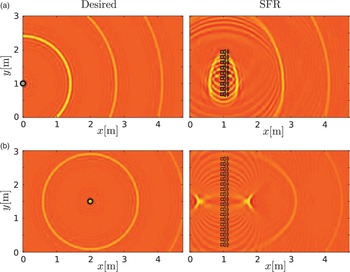
2. Wave field synthesis
WFS [Reference Berkhout6] is a notable principle of reproducing sound fields based on the interior Helmholtz integral equation and its special cases expressed through Rayleigh's I and II integrals [Reference Williams12]. For the sake of space, we only give Rayleigh's I integral, which serves as the essence of WFS with omnidirectional loudspeakers:
 $$P\lpar {\bi r}^{\prime}\comma \; \omega\rpar = -2 \vint_{\partial V_{xy}} \! i\rho_0\omega \, G_\omega\lpar {\bi r}\vert {\bi r}^{\prime}\rpar \, V_n \lpar {\bi r}\comma \; \omega\rpar \, {\rm d}\lpar \partial V_{xy}\rpar . $$
In words, Rayleigh's I integral gives a way of reproducing sound fields that emanate from sources in the half-space z < 0 with a distribution of secondary point sources in the plane z = 0.
Figure 16 illustrates the mentioned principle. The secondary sources are identified through the term G ω(r| r ′), which is the free-field Green's function, and their driving signals are given by the normal component V n ( r , ω) of the particle velocity vector of the desired sound field in the plane z = 0.
The principle of reproducing sound fields in the half-space z > 0 using a planar distribution of secondary point sources in the xy-plane.
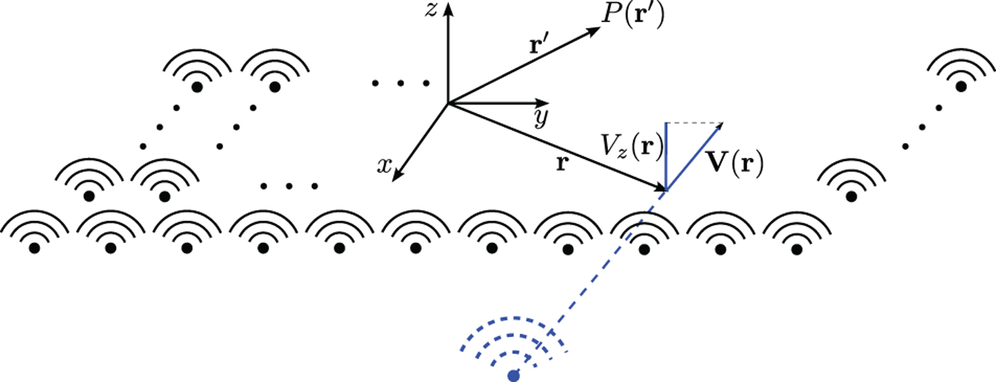
For a system based on Rayleigh's I integral to be practical, one needs a loudspeaker array of finite size (often a single-line array), which mathematically corresponds to approximating the integral in (39) with a finite sum. As a consequence, the WFS reproduction is limited to the frequencies below an aliasing frequency
 $$f_{max} = \displaystyle{c \over 2 \Delta x \sin \alpha_{max}}$$
determined by the loudspeaker spacing Δ x and the maximum radiation angle α max of reproduced sound sources [Reference Berkhout6].
It should be noted that loudspeaker spacing Δ x is the main cause of the spatial aliasing artifacts above the aliasing frequency, irrespective of the reproduction method. One can mitigate the problem to some degree by selecting active loudspeakers [Reference Kolundžija, Faller and Vetterli9,Reference Corteel36,Reference Spors47] or applying a tapering window [Reference Verheijen46].
VII. CONCLUSION
This paper presented a view of sound fields based on the theory of multidimensional signal processing. We saw that point sources generate spherical wave fronts, which become increasingly flatter and weaker the farther they propagate. Such waves are shaped by a PM and an EM, which causes the amplitude to decay. Owing to the Huygens principle, wave fronts can theoretically be sampled and reconstructed with an array of microphones and loudspeakers. This provides a basis for processing wave fields in discrete space and time. We showed that acoustic wave fields are essentially band-limited, and that the spatiotemporal Fourier transform of a point source has a symmetric triangular pattern. This triangle opens and closes as a function of the distance between the source and the sampling axis, and skews according to the average direction of the wave front. If multiple sources are present, they can be separated by applying a 2D filter that matches the spectral triangle of each desired source. They can also be compressed using the principles of digital audio coding and psychoacoustics. Finally, we showed that a wave field can be reconstructed in a listening area with little spatial aliasing, by solving an optimization problem over a discrete set of control points.
Francisco Pinto is a senior researcher at the Centre for Digital Education at the Swiss Federal Institute of Technology (EPFL), Lausanne, Switzerland. He received his Electrical Engineering degree in 2004 from the University of Porto, Portugal, and his Ph.D. in Computer Sciences in 2010 from EPFL. His main research interests are Fourier Acoustics and Signal Processing. He was the recipient of the Calouste Gulbenkian Fellowship in 2006 and the Best Student Paper Award at the IEEE International Conference on Acoustics, Speech, and Signal Processing in 2008.
Mihailo Kolundžija is a research engineer at Sonoview Acoustic Sensing Technologies, Switzerland, and a lecturer at the Swiss Federal Institute of Technology (EPFL). He obtained the PhD and MSc degrees from the EPFL in 2011 and 2007, respectively, under the supervision of Martin Vetterli and Christof Faller. Previously, he received the Dipl.-Ing. degree in Electrical Engineering and Computer Science from the University of Novi Sad, Serbia, in 2004. His work and interests span the areas of spatial sound capture and reproduction, room acoustics, psychoacoustics, speech processing, tomographic imaging, and image processing.
Martin Vetterli received the Dipl. El.-Ing. degree from Eidgenössische Technische Hochschule (ETHZ) in 1981, the Master of Science degree from Stanford University in 1982, and the Doctorat ès Sciences degree from Ecole Polytechnique Fédérale de Lausanne (EPFL) in 1986.
After his dissertation, he was an Assistant and Associate Professor in Electrical Engineering at Columbia University in New York, and in 1993, he became an Associate and then Full Professor at the Department of Electrical Engineering and Computer Sciences at the University of California at Berkeley. In 1995, he joined the EPFL as a Full Professor. He held several positions at EPFL, including Chair of Communication Systems and founding director of the National Competence Center in Research on Mobile Information and Communication systems (NCCR-MICS). From 2004 to 2011 he was Vice President of EPFL for international affairs, and from 2011 to 2012, he was the Dean of the School of Computer and Communications Sciences. Since January 2013 he is President of the National Research Council of the Swiss National Science Foundation.
He works in the areas of electrical engineering, computer sciences and applied mathematics. His work covers wavelet theory and applications, image and video compression, self-organized communications systems and sensor networks, as well as fast algorithms, and has led to about 150 journals papers, as well as about 30 patents that led to technology transfer to high-tech companies and the creation of several start-ups.
He is the co-author of three textbooks, “Wavelets and Subband Coding” (with J. Kovacevic, Prentice-Hall, 1995), “Signal Processing for Communications” ( P. Prandoni, EPFL Press, 2008) and “Foundations of Signal Processing” (with J. Kovacevic and V. Goyal, Cambridge University Press, 2014). These books are available in open access, and his research group follows the reproducible research philosophy.
His work won him numerous prizes, like best paper awards from EURASIP in 1984 and of the IEEE Signal Processing Society in 1991, 1996 and 2006, the Swiss National Latsis Prize in 1996, the SPIE Presidential award in 1999, the IEEE Signal Processing Technical Achievement Award in 2001 and the IEEE Signal Processing Society Award in 2010. He is a Fellow of IEEE, of ACM and EURASIP, was a member of the Swiss Council on Science and Technology (2000-2004), and is a ISI highly cited researcher in engineering.


 Open access