

I. INTRODUCTION
Emotional voice conversion (VC) is a kind of VC technique for converting prosody in speech, which can represent different emotions while keeping the linguistic information unchanged. In a voice, the spectral and fundamental frequency (F0) features can affect the acoustic and prosodic features, respectively. So far, spectral mapping mechanisms have achieved tremendous success in VC tasks [Reference Nakashika, Takiguchi and Minami1–Reference Toda4], while, how to effectively generate prosody in the target voice remains a challenge. We know that prosody plays an important role in conveying various types of non-linguistic information that represent the mood of the speaker. Previous studies have shown that F0 is an important feature for prosody conversion that is affected by both short- and long-term dependencies, such as the sequence of segments, syllables, and words within an utterance [Reference Ribeiro and Clark5]. However, it may be difficult to apply conventional deep learning-based VC to F0 conversion using simple representations of F0, such as dynamic features (delta F0).
In recent years, it has been shown that the continuous wavelet transform (CWT) method can effectively model F0 in different temporal scales and significantly improve speech synthesis performance [Reference Vainio6]. For this reason, Suni et al. [Reference Suni7] applied CWT to intonation modeling in hidden Markov model (HMM) speech synthesis. Ming et al. [Reference Ming, Huang, Dong, Li, Xie and Zhang8] used CWT in F0 modeling within the non-negative matrix factorization (NMF) model for emotional VC. Our earlier work [Reference Luo, Chen, Takiguchi and Ariki9] systematically captured the F0 features of different temporal scales using adaptive scales CWT (AS-CWT), which transforms F0 features into high-dimensional CWT-F0 features containing more specifics. Conventional emotional VC tasks are focusing on converting one emotional voice to another fixed emotional voice. However, in the real world, the emotional voice is complex, with different prosody factors, and evolves over time. Thus, in order to better represent the interactions of components in emotional voices and generate a greater variety of representations of F0 features. In this study we want to go one step further and generate more emotional features using the cross-wavelet transform (XWT) [Reference Torrence and Compo10]. The XWT method is a technique that characterizes the interaction between the wavelet transform of two individual time-series, which was first introduced by Hudgine et al. [Reference Hudgins, Friehe and Mayer11] and has been used in many areas such as economic analysis [Reference Cai, Tian, Yuan and Hamori12], geophysical time series [Reference Grinsted, Moore and Jevrejeva13] or electrocardiogram signals analysis [Reference Banerjee and Mitra14]. Moreover, to improve the emotional VC effect with a limited amount of training data, we propose a new generative model, which will be described followed.
Many deep learning-based generative models exist including Restrictive Boltzmann Machine [Reference Smolensky15], Deep Belief Networks [Reference Hinton, Osindero and Teh16], Variational Autoencoder (VAE) [Reference Kingma and Welling17] and Generative Adversarial Nets (GAN) [Reference Goodfellow18]. Most of them have been applied in spectral conversion. Nakashika et al. [Reference Nakashika, Takashima, Takiguchi and Ariki19] proposed a VC method using DBNs to achieve non-linear deep transformation. Hsu et al. [Reference Hsu, Zhang and Glass20] applied a convolutional VAE to model the generative process of natural speech. Kaneko et al. [Reference Kaneko, Kameoka, Hiramatsu and Kashino21] used GAN in sequence-to-sequence voice conversion. The illustration of the structure of VAE [Reference Kingma and Welling17] and GAN [Reference Goodfellow18] are shown in Fig. 1(2) and Fig. 1(2), respectively.

Fig. 1. Illustration of the structure of VAE [Reference Kingma and Welling17], GAN [Reference Goodfellow18] and the proposed VA-GAN. Here x and x' are input and generated features. z is the latent vector and t are target features. E, G, D are the encoder, generative, and discriminative networks, respectively. h is the latent representation processed by encoder network. y is a binary output which represents real/synthesized features.
Owing to the success of VAE and GAN in VC tasks, Hsu et al. [Reference Hsu, Hwang, Wu, Tsao and Wang3] proposed the Variational Autoencoding Wasserstein Generative Adversarial Networks (VAW-GAN) for non-parallel VC tasks, which combined VAE with Wasserstein GAN [Reference Arjovsky, Chintala and Bottou22]. In this study, different from the VAW-GAN [Reference Hsu, Hwang, Wu, Tsao and Wang3], which is mainly used in non-parallel data voice conversion, the main task for emotional VC is how to maintain good model training using limited parallel emotional data and the simple representations of F0 features. Therefore, we propose an emotional VC framework that combines VAE with a conditional GAN [Reference Isola, Zhu, Zhou and Efros23], which is named VA-GAN. The effectiveness of GAN is due to the fact that an adversarial loss forces the generated data to be indistinguishable from real data. This is particularly powerful for generation tasks, but the training of the GANs is difficult and unstable. This leads to results in which the generated voice is unnatural and of bad quality. Another popular generative model, VAE, suffers from the problem of fuzzy sound, which is caused by injected noise and imperfect element-wise measures, such as the squared error. Thus, by combining the VAE and GAN models, the VAE can provide the efficient approximated posterior inference of the latent factors for improved GAN learning. Meanwhile, GAN can enhance VAE with an adversarial mechanism for leveraging generated samples.
As shown in Fig. 1(3), our VA-GAN consists of three parts: (1) the encoder network E, which maps the data sample x to a latent representation h, (2) the generative network G, which generates features x′ from the latent representation h, (3) and the discriminative network D, which distinguishes real/fake (t/x′) features. Here, we use the t and x′ to represent the target and converted emotional voice. These three parts are seamlessly cascaded together, and the whole pipeline is trained end-to-end.
In summary, we show two major advantages of using our method. First, we employ the XWT to combine CWT-F0 features of different emotions. By doing so, we can obtain the XWT-F0 features and reconstruct them to various F0 features combined with different emotions, offering a huge advantage in emotional voice synthesis. Additionally, the XWT-F0 features can also increase the representations of F0 features which can improve the emotional VC. Second, we designed VA-GAN based on VAE and GAN architectures to process the emotional VC tasks, which can effectively avoid over-smoothing as well as capture a highly non-linear network structure, by simultaneously integrating XWT-F0 features into network representation learning.
In the remaining part of this paper, feature extraction and processing are introduced in Section II. Then, we describe our proposed training model (VA-GAN) in Section III. Section IV gives the detailed process stages of our experimental evaluations, and Section V presents our conclusions.
II. FEATURE EXTRACTION AND PROCESSING
It is well known that prosody is influenced both at a supra-segmental level, by long-term dependencies, and at a segmental-level, by short-term dependencies. And, as has been proven in our recent studies [Reference Luo, Chen, Takiguchi and Ariki9,Reference Luo, Chen, Nakashika, Takiguchi and Ariki24], the CWT can effectively model F0 in different temporal scales and significantly improve the system performance. So, in the proposed method, we adopt CWT to decompose the one-dimensional F0 features into high-dimensional CWT-F0 features, and then, use the XWT to combine the CWT-F0 features of different emotions. In the remaining part of this section, we will present the basic CWT and XWT theories, and illustrate how to use them in carrying out emotional VC.
A) Continuous wavelet transform
In what follows, L 2(ℝ) denotes the set of square-integrable functions, which satisfy  $\int_{-\infty }^{+\infty }\left \vert x(t) \right \vert^{2}dt \lt \infty$. Given a time series f 0(t) ∈ L 2(ℝ), its continuous wavelet is, in respect to the mother wavelet ψ ∈ L 2(ℝ), defined as
 $$\psi_{s,\tau}=s^{-1/2}\psi_{0} \left(\displaystyle{{t-\tau}\over{s}}\right)dt, s,\tau\in{\open R}, s\neq 0,$$
where s is the scaling factor (which controls the width of the wavelet), and τ is the translating factor (which decides the location of the wavelet). (s −1/2) is used for normalization, which can ensure unit variance of the wavelet and ‖ψ s,τ‖2 = 1. Thus, the CWT of an input signal f 0(t) can be written as
 $$\eqalign{W_{f_{0};\psi}\left(s,\tau\right )&= \left \langle f_{0}(t),\psi _{s,\tau}(t) \right \rangle=\int_{-\infty }^{\infty }f_{0} \left(t \right )\psi_{s,\tau}(t)dt \cr & = s^{-1/2}\int_{-\infty }^{\infty }f_{0} \left(t \right )\psi_{0} \left(\displaystyle{{t-\tau}\over{s}}\right )dt}$$
 $$\psi_{0} (t) = \displaystyle{{2}\over{\sqrt{3}}}\pi^{-1/4} \left(1-t^{2}\right)e^{-t^{2}/2},$$
where f 0(t) is the input signal and mother wavelet ψ(t) used in our model is the Mexican hat mother wavelet [Reference Torrence and Compo10]. The wavelet transform can give us information simultaneously on time-frequency space by mapping the original time series into the function of s and τ. Because both s and τ are real values and vary continuously,  $W_{f_{0};\psi }(s,\,\tau )$ is named a CWT. To be a mother wavelet of the CWT, ψ(t) must fulfill admissibility conditions [Reference Daubechies25], which can be written as follows:
 $$0 \lt C_{\psi }=\int_{-\infty }^{+\infty}\displaystyle{{\vert\hat\psi(f)\vert^{2}}\over{\left \vert f \right \vert}} \lt +\infty,$$
where  $\hat \psi (f)$ is the Fourier transform of the mother wavelet ψ(t) and f is the Fourier frequency. It is clear that C ψ is independent of f and determined only by the wavelet ψ(t). This means that C ψ is a constant for each given mother wavelet function. Thus, we can reconstruct f 0(t) using its CWT, $W_{f_{0};\psi }( s,\,\tau )$, by inverse function as follows:
 $$\eqalign{f_{0}(t) & = \displaystyle{{1}\over{C_{\psi}}}\int_{0}^{+\infty } \left [ \int_{-\infty }^{+\infty }W_{f_{0};\psi} \left(s,\tau\right ) \psi _{s,\tau}(t)d\tau\right ]\displaystyle{{ds}\over{s^{2}}}, \cr & \qquad s \gt 0}$$
In this way, we can decompose F0 features f 0(t) to the CWT-F0 features  $W_{f_{0};\psi }(s,\,\tau )$ and reconstruct them back to F0 features. Therefore, we have reason to believe that F0 and CWT-F0 are two different representations of the same mathematical entity. Fig. 2(2) shows the examples of CWT features decomposed from the F0 features of source and target emotional voices. In this figure, we show the parts of the scales that can represent the sentence, phrase, word, syllable, and phone levels, respectively. Moreover, the energy of the examined time series is preserved by its CWT in the sense that
 $$\eqalign{\left\Vert f_{0}(t) \right\Vert^{2} & =\displaystyle{{1}\over{C_{\psi}}}\int_{0}^{+\infty} \left[\int_{-\infty }^{+\infty }\vert W_{f_{0};\psi} \left(s,\tau\right)\vert^{2} \psi_{s,\tau}(t)d\tau\right]\displaystyle{{ds}\over{s^{2}}}, \cr & \qquad s \gt 0}$$
where ‖f 0(t)‖2 is defined as the energy of f 0(t), and  $\vert W_{f_{0};\psi }( s,\,\tau )\vert^{2}$ is defined as a wavelet power spectrum that can interpret the degree of local variance of f 0(t) scale by scale. The examples of wavelet power spectrum of the source and target CWT-F0 features are represented by the first pan and the second pan of Fig. 2(3).
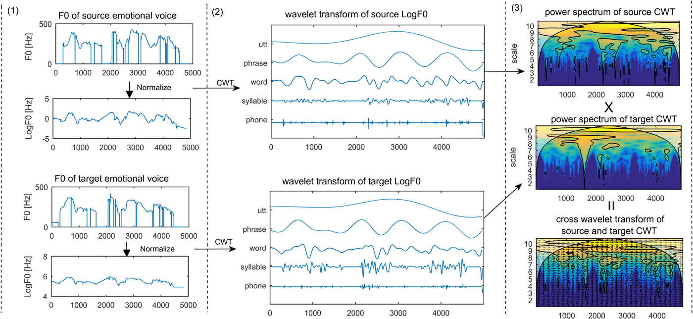
Fig. 2. (1) Linear interpolation and log-normalized processing for source and target emotional voice. (2) The CWT for normalized LogF0 contours, the top pan and bottom pan show five examples of the different level's decomposed CWT-F0 features of the source and target F0, respectively. (3) First and second pans show the continuous wavelet spectrums of the source and target CWT-F0 features and the bottom pan represents the cross-wavelet spectrums of the two CWT-F0 features. The relative phase relationship is shown as arrows in the cross-wavelet spectrum (with in-phase pointing right (→), anti-phase pointing left (←), and source emotional features leading target emotional features by 90° pointing straight down.
B) Cross wavelet transform
Given two time series,  $f_{0_{x}}(t)$ and $f_{0_{y}}(t)$, with their CWT features, W x, and W y, XWT is defined as $W_{xy;\psi }(s,\,\tau )=W_{x;\psi }(s,\,\tau )W_{y;\psi }\ast (s,\,\tau )$, where * denotes complex conjugation. And their cross-wavelet power spectrum is accordingly written as
 $$\vert W_{xy;\psi}(s,\tau)\vert^{2}=\vert W_{x;\psi}(s,\tau)\vert^{2}\vert W_{y;\psi}\ast(s,\tau)\vert^{2}.$$
An example of the cross-wavelet power spectrum is shown in the last pan of Fig. 2(3). The XWT of a two-time series depicts the local covariance between them at each time and frequency and shows the area in the time-frequency space where the two signals exhibit high common power. Thus, we can do the cross-transform for different emotional voices to synthesize the new XWT-F0 features, and then reconstruct them to new synthesized F0 features. The new synthesized F0 features can be used in processing a new emotional voice or increasing the training data for emotional VC training.
C) Applying CWT and XWT in F0 features extraction
The STRAIGHT [Reference Kawahara26] is frequently used to extract features from a speech signal. Generally, the smoothing spectrum and instantaneous-frequency-based F0 are derived as excitation features for every 1 ms from the STRAIGHT. As shown in Fig. 2, there are three steps for processing the XWT-F0 features.
1) To explore the perceptually-relevant information, F0 contour is transformed from the linear to logarithmic semitone scale, which is referred to as logF0. As shown in the first pan and second pan of Fig. 2(2), the F0 features extracted by STRAIGHT from the source and target emotional voice are discrete. As the wavelet method is sensitive to the gaps in the F0 contours, we must fill in the unvoiced parts in the logF0 via linear interpolation to reduce discontinuities in voice boundaries. Finally, we normalize the interpolated logF0 contour to zero mean and unit variance. Examples of interpolated LogF0 contours of source and target emotional voice are depicted in the second and last pan of Fig. 2(2), respectively.
2) Then, we adopt CWT to decompose the continuous logF0 into 30 discrete scales, each separated by one-third of an octave. F0 is thus approximately represented by 30 separate components given by [Reference Luo, Chen, Nakashika, Takiguchi and Ariki24]
(8)where i = 1,…,30 and τ 0 = 1 ms. In Fig. 2 (2), we just show five examples of the decomposed CWT-F0 features which represent the utterance, phrase, word, syllable and phone levels, respectively. $$W_{i}(f_{0})(t)=W_{i}(f_{0})(2^{(i/3)+1}\tau _{0},t) \left((i/3)+2.5 \right)^{^{-5/2}},$$
3) Finally, we do the XWT for CWT-F0 features of the two emotional voices. First, we process the power spectrums of the source and target CWT-F0 features, and then use the cross-wavelet function to combine the two CWT-F0 features to cross-wavelet F0 features (XWT-F0). Fig. 2(3) shows the power spectrums of CWT-F0 features and the XWT-F0 feature. The XWT-F0 features can be used for generating the combinative emotional voice. Moreover, they can also be used for increasing the training data of the emotional VC tasks.

III. TRAINING MODEL: VA-GAN
A) Background: VAE and GAN
1) Variational autoencoder
VAE defines a probabilistic generative process between observation x and latent variable h as follows:
 $${\bf z} \sim Enc({\bf x})= q_{\bi \phi}({\bf h}\vert{\bf x}), {\tilde{\bf x}}\sim Dec({\bf h})= p_{\bi \theta}({\bf h}\vert{\bf x}),$$
where (Enc) represents encode networks that encode a data sample x to a latent representation h and decode networks (Dec) decode the latent representation back to data space. In the VAE, the recognition model  $q_{\bm {\phi }}({\bf h \vert x})$ approximates the true posterior $p_{\bm {\theta }}({\bf h}\vert{\bf x})$. The VAE regularizes the encoder by imposing a prior over the latent distribution $p_{\bm {\theta }}({\bf h})$, which is assumed to be a centered isotropic multivariate Gaussian $p_{\bm {\theta }}({\bf h})\sim N({\bf h};{\bf 0},\,{\bf I})$. The VAE loss $L_{\bm {\theta },\,\bm {\phi };{\bf x}}$ is minus the sum of the expected log-likelihood L like (the reconstruction error) and a prior regularization term L prior represented as:
 $$L_{\bi \theta},{\bi \phi};{\bi x} =-E_{q_{\bi \phi}}({\bf h} \vert {\bf x})[\log \displaystyle{{{p_{\bi \theta}}({\bf x} \vert {\bf h})p_{\bi \theta}(h)}{q_{\bi \phi}({\bf h} \vert {\bf x})}}]=L_{like}+L_{prior},$$
 $$L_{like}=-E_{q_{\bi \phi}}({\bf h} \vert {\bf x})[\log p_{\bi \theta}({\bf x} \vert {\bf h})],$$
 $$L_{prior} = KL(q_{\bi \phi}({\bf h}\vert {\bf x})\Vert p_{\bi \theta}({\bf h})),$$
where KL is the Kullback-Leibler divergence. We use the KL loss to reduce the gap between the prior P(h) and the proposal distributions. The loss of KL is only related to the encoder network Enc. It represents whether or not the distribution of the latent vector is under expectation. Here, we want to optimize  $L_{\bm {\theta ,\phi ;x}}$ in respect to θ and ϕ.
In the VC area, VAE is used to learn latent representations of speech segments to model the conversion process. Refer to applying the VAE in the non-parallel VC tasks proposed by Hsu et al. [Reference Hsu, Zhang and Glass20]. We can also apply them in the emotional VC with parallel data. If we want to estimate the latent representations for each emotional feature, we can estimate latent attributes by taking the mean latent representations as shown in Fig. 3(a). Supposing we want to convert the prosody attribute of a speech segment  ${\bf x}_{A}^{i}$, from being a source emotional voice e A to being a target emotional voice e B. Given the means of latent attribute representations ${\bi \mu}_{e_{A}}$ and ${\bi \mu}_{e_{B}}$ for emotional e A and e B, respectively, we can transform the latent attribute computed as ${\bf v}_{e_{A}\rightarrow e_{B}}={\bi \mu}_{e_{B}}-{\bi \mu}_{e_{A}}$. We can then modify the speech $x_{A}^{i}$ as follows:
 $${\bf h}_{A}^{i} \sim q_{\bi \phi}({\bf h}\vert{\bf x}_{A}^{(i)}),$$
 $${\bf h}_{B}^{(i)} ={\bf h}_{A}^{(i)}+{\bf v}_{e_{A}\rightarrow e_{B}},$$
 $${\bf x}_{B}^{(i)} \sim p_{\bi \theta}({\bf x}\vert{\bf h}_{B}^{(i)}),$$
Figure 3(b) shows an illustration of the conversion phase.

Fig. 3. (left) Examples of processing the latent representations for emotion A and emotion B using Variational Autoencoder (VAE). (right) Examples of modifying the emotional voice from emotion A to emotion B.  ${\bi \mu}_{e_{A}}$ and ${\bi \mu}_{e_{B}}$ represent the means of latent attribute representations for emotional e A and e B, respectively. q bmϕ and p bmθ mean the encode and decode functions, respectively. ${\bf x_{A}}^{i}$ and ${\bf x_{B}}^{i}$ represent the speech segment of emotion A and emotion B.
2) Generative adversarial networks
GAN has obtained impressive results for image generation [Reference Denton27,Reference Radford, Metz and Chintala28], image editing [Reference Zhao, Mathieu and LeCun29], and representation learning [Reference Salimans, Goodfellow, Zaremba, Cheung, Radford and Chen30]. The key to the success of the GAN is learning a generator distribution P G(x) that matches the true data distribution. It consists of two networks: a generator, G, which transforms noise variables z ~ P Noise(z) to data space x = G(z) and a discriminator D. This discriminator assigns probability p = D(x) when x is a sample from the P Data(x) and assigns probability 1−p when x is a sample from the P G(x). In a GAN, D and G play the following two-player minimax game with the value function V (G, D):
 $$\eqalign{\min\limits_{G} \max\limits_{D}V(D,G) & = E_{{\bf x}\sim p_{data}}[\log D({\bf x})] \cr & \quad + E_{z\sim p_{{\bf z}}({\bf z})}[\log(1-D(G({\bf z})))]}.$$
This enables the discriminator, D, to find the binary classifier that provides the best possible discrimination between true and generated data and simultaneously enables the generator, G, to fit P Data(x). Both G and D can be trained using back-propagation.
The effectiveness of GAN is due to the fact that an adversarial loss forces the generated data to be indistinguishable from real data. This is particularly powerful for image generation tasks, and, owing to GAN's ability to generate a high-fidelity image which can mitigate the over-smoothing problem caused in the low-level data space when converting the speech features. GAN models have also begun to be applied in speech synthesis [Reference Kaneko, Kameoka, Hojo, Ijima, Hiramatsu and Kashino31] and VC [Reference Kaneko, Kameoka, Hiramatsu and Kashino21].
Figure 4 gives an overview of the training procedure when using the GAN model for VC tasks. In conventional studies [Reference Kaneko, Kameoka, Hiramatsu and Kashino21,Reference Kaneko, Kameoka, Hojo, Ijima, Hiramatsu and Kashino31], in the VC tasks, they used not only a sample from the “G” but also a sample from the “C” as the discriminator input. Here, “C” represents the conversion function. This is because the samples converted from the source voice are more similar to the target voice than the samples generated by noise. Thus, using the converted samples can improve the updating of D. The value function used in VC is rewritten as
 $$\eqalign{\min\limits_{G} \max\limits_{D}V(D,G) & = E_{x\sim p_{data}}[\log D({\bf x})] \cr & \quad + E_{z\sim p_{{\bf z}}({\bf z})}[\log(1-D(G({\bf x,z})))] \cr & \quad + E_{z\sim p_{{\bf z}}({\bf z})}[\log(1-D(C({\bf x})))].}$$
Fig. 4. Illustration of calculating the loss of GAN in voice conversion.
B) VA-GAN training model
As described above, there is a clear and recognized way to evaluate the quality of the VAE model. However, due to the injected noise and imperfect reconstruction, the generated samples are much more blurred than those coming from GAN. GAN models tend to be much more finicky to train than VAE and, therefore, can obtain a high-fidelity image. But, in practice, the GAN discriminator D can distribute the “real” and “fake” images easily, especially at the early stage of the training process. This will cause the problem of an unstable gradient of G when training GAN [Reference Arjovsky, Chintala and Bottou22,Reference Arjovsky and Bottou32]. To solve the problems associated with VAE and GAN models, we combine the VAE and GAN models to form one advanced model, which we named VA-GAN. As shown in Fig. 5, our model contains an encoder (Enc), conversion function (C:x → y) and a discriminator (D). To resolve the instability of training GAN, we extract the representative features from a pre-trained Enc. Also, we can obtain better results when using the latent representation (h) from the encoder Enc. When dealing with the training of emotional VC, every two sets of labeled and paired feature matrices were sampled from domains source emotional voice X and target emotional voice Y , respectively. For the conversion function C:x → y and its discriminator D with pre-trained Enc, we express the objective of adversarial loss as:
 $$\eqalign{L_{GAN}(C,D,X,Y) &=E_{{\bf y}\sim P_{data}({\bf y})}[\log D({\bf y},{\bf x})] \cr &\quad + E_{{\bf x}\sim P_{data}({\bf x})}[\log (1-D(C(Enc({\bf x}))))].}$$
Fig. 5. Illustration of calculating the loss of VA-GAN.
The goal of emotional VC is to learn a converted emotional voice distribution P C(x) that matches the target emotional voice distribution P data(y). Equation (18) enables D to find the binary classifier that provides the best possible discrimination between a true and a converted voice and simultaneously enables the function “C” to fit the P data(y). We also mix the GAN objective with a traditional L1 distance loss as:
 $$L_{1}(C) =E_{{\bf x,y,z}}[\left \Vert y-C({\bf x,z})\right \Vert_{1}].$$
Our final objective is maximized and minimized with respect to “D” and “C”, respectively.
 $$G^{\ast }=arg\,\max_{D}\,\min_{C}\,L_{GAN}(C,D,X,Y) +\lambda L_{1}(C).$$
 In the VAE for the emotional VC, emotion-independent encoder (Enc) infers a latent content z ~ Enc(x), and then the emotion-dependent decoder (Dec) mixes z with an emotion-specific variable y to reconstruct the input as a variational approximation:  $\tilde {x}\approx Dec(z,\,y)$. The aim of a VAE is to learn a reduced representation of the given data. Consequently, feature spaces learned by the VAE are powerful representations for reconstructing the P data(y) distribution. However, VAE models tend to produce unrealistic, blurry samples [Reference Dosovitskiy and Brox33], and Zhao et al. [Reference Zhao, Song and Ermon34] provide a formal explanation for this problem. To solve the blurriness issue, similar to some VAE and GAN combined models [Reference Larsen, Sønderby, Larochelle and Winther35,Reference Rosca, Lakshminarayanan, Warde-Farley and Mohamed36], we replaced the reconstruction error term from equation (11) with a reconstruction error expressed in the discriminator D. To achieve this, we let D l(x) denote the hidden representation of the lth layer of the discriminator, and we introduce a Gaussian observation model for D l(x) with mean $D_{l}(\tilde {{\bf x}})$ and identity covariance:
 $$p(D_{l}({\bf x})\vert{\bf z})=N(D_{l}({\bf x})\vert D_{l}(\tilde{{\bf x}}),{\bf I}),$$
where  $\tilde {{\bf x}}\sim Dec({\bf h})$ in equation (9) is now the sample from the conversion function “C” of “x”. We can now replace the VAE error of equation (11) with
 $$L_{like}^{D_{l}}=-E_{q({\bf z\vert x})}[\log p(D_{l}({\bf x})\vert{\bf z})].$$
The goal of our approach is to minimize the following loss function:
 $$L=L_{GAN}+L_{like}^{D_{l}}+L_{prior}+\lambda L_{1}(C),$$
where λ controls the relative importance of the distance loss function. The details of how to train VA-GAN are indicated in Algorithm 1.
Algorithm 1 Training procedure of VA-GAN

Throughout the training process, conversion functions C is optimized to minimize the VAE loss and to learn the converted emotional voice, which cannot be distinguished from the target emotional voice by corresponding discriminators D.
IV. EXPERIMENTS
In our experiments, we used a database of emotional Japanese speech constructed in a previous study [Reference Kawanami, Iwami, Toda, Saruwatari and Shikano37]. In the database, there is a total of 50 different kinds of content sentences, and each sentence was read in four different emotions (angry, happy, sad, and neutral) by the same speaker. Thus, there 50 × 4 × N waveforms in the database, where N is the number of speakers, the waveforms were sampled at 16 kHz.
In the emotional VC experiment, we classified the three datasets into the following voice types: neutral to angry voices (N2A), neutral to sad voices (N2S), and neutral to happy voices (N2H). For each data set, 40 sentences were chosen as basic training data and 10 sentences were chosen for the VC evaluation.
To do the evaluation of prosody conversion using our proposed VA-GAN method, we compared the results with several state-of-the-art methods. Logarithm Gaussian (LG) normalized transformation is often used for F0 features conversion in deep learning VC tasks [Reference Liu, Zhang and Yan38,Reference Chen, Ling, Liu and Dai39]. Our previous work [Reference Luo, Chen, Takiguchi and Ariki9] dealt with a NNs model that used the pre-trained NNs to convert the CWT-F0 features. We also compared VA-GAN with the GAN and VAE.
Before applying the XWT-F0 features to the emotional VC, we need to calculate the correlates of different emotional voices. In other words, we do the cross-matching of each two emotional voices for the same content by the same speaker, which will result in six datasets (N, A), (N, S), (N, H), (A, H), (A, S), (H, S). For each dataset, we do the XWT to synthesize the XWT-F0 features, and then reconstruct them to the F0 features that can be used for generating the complex emotional voice. Finally, we carry out a subjective experiment to decide the synthesized emotional voices that belong to which kind of emotion (neutral, angry, happy, sad, and unknown). Here, due to some generated emotional voices may sound strange, we added the unknown option.
To evaluate the effectiveness of XWT-F0 features used as the increased training data for emotional VC, we carry out the experiments by adding the XWT-F0 features, which are selected by the subjective experiment, to the corresponding CWT-F0 features to increase the training data.
Moreover, to evaluate the relationship between different data size and the conversion methods described above, we conducted our experiment using a larger open database [Reference Sonobe, Takamichi and Saruwatari40], which contains 100 sentences for each emotional voice. Among them, 80 sentences were chosen for training data and the existing 20 sentences were chosen for the testing data. In these experiments, the spectral features were converted using the same models as their CWT-F0 features training model (For the NNs model, we used the DBNs model to train spectral features, which has been proposed in [9]).
A) Selecting cross wavelet features
To evaluate the synthesized emotional voice with the XWT-F0 features, we devised a subjective evaluation framework as shown in Fig. 6. We first perform CWT on the neutral, angry, happy, and sad voice to decompose their F0 contours into CWT-F0 features. Then do the XWT for each pair of emotional CWT-F0 features, to process the XWT-F0 features. Then we reconstruct the XWT-F0 features to F0 features to synthesize the complex emotional voice. Then we ask 10 subjects to listen and choose the emotion that is close to the synthesized speeches.

Fig. 6. The listening experiment setup for evaluating emotional voice generated by different XWT-F0 features. The small letters in the lower right of CWT-F0 and XWT-F0 represent the emotion. For instance, (n) and (a) represent the neutral and angry. (n,a) represents the XWT-F0 features generated by CWT-F0 features of angry and neutral.
Figure 7 shows the similarity to different emotions of the synthesized emotional voices using the different XWT-F0 features. For example, XWT (n, a) represents the synthesized emotional voice cross transformed with the neutral and angry CWT-f0 features. As the figure shows, the emotional voice generated from the neutral and sad voices XWT (n, s) got the most votes for the similarity to a sad voice. The voting results of XWT (n, a) and XWT (a, s) indicate that the angry voice can be generated by angry and sad voice or angry and neutral voice. However, not all the generated emotional voices are good. For instance, the happy voice can be generated by XWT (n, h), but half of the subjects voted for the XWT (n, h) generated voice over the neutral voice. The XWT (h, s) and XWT (a, h) got the most votes for unknown, which means there was a strange prosody of the generated emotional voice.
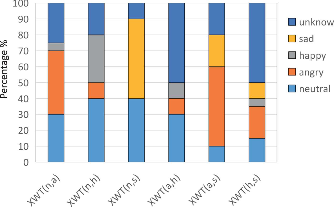
Fig. 7. Similarity to different emotional voices (neutral, angry, happy, and sad) of synthesized emotional voices with different XWT-F0 features.
In summary, depending on the emotional classification results of the emotional voice generated by the XWT-F0 (n, s), XWT-F0 (n, a), XWT-F0 (a, s) and XWT-F0 (n, h) features, we can use XWT-F0 (n, s) features as the CWT-F0 features of a sad voice, XWT-F0 (n, a) and XWT-F0 (a, s) as an angry voice, and the XWT-F0 (n, h) as a happy voice. Then, we can use both CWT-F0 features and their corresponding XWT-F0 features as the input training data, and the output is the CWT-F0 features.
B) Training procedure
Table 2 details the network architectures of the encoder (Enc), the converter (C) and discriminator (D). The symbols ↓ and ↑ indicate down sampling and up sampling, respectively. To upscale and downscale, we respectively used convolutions and backward convolutions with stride 2.
In the converter (C), similar to the generator used in Johnson et al. [Reference Johnson, Alahi and Fei-Fei41], we use batch normalization (BNorm) [Reference Ioffe and Szegedy42] and all convolutional layers are followed by ReLU nonlinearities [Reference Maas, Hannun and Ng43] with the exception of the output layer. The C contains one stride-2 convolution to downsample the input, followed by two residual blocks [Reference He, Zhang, Ren and Sun44], and two fractionally-strided upsampling convolutional layers with stride 1/2.
For discriminator (D), we refer to a convolutional PatchGAN classifier [Reference Li and Wand45] but use a smaller patch size. The patch size at which the discriminator operates is fixed at 20 × 20, and two stride-2 convolutions and a fully connected layer make up the (D). After the last layer, we apply a sigmoid activation function to obtain a probability for sample classification.
When training the (Enc) (C) and (D), we use the Adam optimizer [Reference Kinga and Adam46] with a mini-batch of size 8, which represents 8 input matrices (30 × 30), including 8 × 30 frames. The learning rate was set to 0.0002 for the Enc and C, and 0.0001 for the D, respectively. The momentum term was set to 0.5.
To clarify the characteristics of our framework with VA-GAN, as described above, we implemented three kinds of generative networks for comparison. The detailed units of the NNs are set to [32, 64, 64, 32]. The compared VAE model consists of the E and C, while the compared GAN model consists of the C and D, which are used in VA-GAN.
C) Objective experiment
To evaluate F0 conversion, we used the root-mean-square error (RMSE) which is defined as:
 $$RMSE=\sqrt{\displaystyle{{1}\over{N}}\sum_{i=1}^{N} \left( \left(F0_{i}^{t} \right)- \left(F0_{i}^{c} \right) \right)^2},$$
where  $F0_{i}^{t}$ and $F0_{i}^{c}$ denote the target and the converted interpolated F0 features, respectively. A lower F0-RMSE value indicates a smaller distortion or predicting error. Unlike the RMSE evaluation function used in one previous study [Reference Ming, Huang, Dong, Li, Xie and Zhang8], which evaluated the F0 conversion by calculating logarithmic scaled F0, we used the target interpolated F0 and converted interpolated F0 of a complete sentence including voiced and unvoiced (0 value), to calculate the RMSE values. Due to the alignment preprocessing in the parallel data, we used the unvoiced part of the source F0 in the converted F0. Considering that F0-RMSE evaluates complete sentences that contain both voiced and unvoiced F0 features instead of the voiced-logarithmic scaled F0, the RMSE values are expected to be high. For emotional voices, the unvoiced features also include some emotional information, such as the pause in a sentence which can sometimes express nervousness or some other negative emotion. Therefore, we choose the F0 of complete sentences for evaluation as opposed to only voiced logarithmic-scaled F0.
As shown in Table 1, LG represents the conventional linear F0 conversion method using F0 features, directly. NNs, VAE, and GAN represent the comparison method using CWT-F0 features only. “+” represents using both the CWT-F0 features and the corresponding selected XWT-F0 features for the training model. As the results indicated, the conventional linear conversion LG has almost no effect in all the emotional VC datasets. The other four methods can affect the conversion of all emotional voice datasets. In addition, the GAN and VA-GAN can obtain significant improvement in F0 conversion. That proves that GAN and our proposed VA-GAN are effective in mapping emotional VC. Comparing the NN and NN+, VAE and VAE+, GAN and GAN+, and VA-GAN and VA-GAN+, we can see that adding the XWT-F0 features cannot improve the GAN model, but doing so can improve the training effectiveness for NN, VAE and the proposed VA-GAN training model.
Table 1. F0-RMSE results for different emotions. N2A, N2S and N2H represent the datasets from neutral to angry, sad and happy voice, respectively. (40) and (80) denote the number of training examples. “+” means using both the CWT-F0 features and selected XWT-F0 features for training model. U/V-ER represents the unvoiced/voiced error rate of the proposed method

Comparing the results of the small size training data and the larger size training data shown in Table 1, The RMSE of NN, GAN, and VAE increase significantly when using the smaller training data size, which means the conversion effect degrades. On the other hand, the RMSE of VA-GAN increased only a little when using a smaller data size, which shows the strength of VA-GAN when using limited training data.
Figure 8 shows the spectrograms of the source voice, target voice, and converted voices with different methods. The converted emotional voices are reconstructed by both converted F0 features and converted spectral features using STRAIGHT.

Fig. 8. Spectrograms of source voice, target voice and converted voices reconstructed by converted spectral features and F0 features using different methods.
As discussed above, the RMSE values obtained using GAN without VAE are also slightly better than NNs model. However, as shown in the Figure 8(D), there is a significant loss in the high-frequency part of the spectrogram of the converted voice. We predict this is due to the fact that, unlike normal object image generation, the dissimilarities between the source and target emotional voices are very small. Therefore, without VAE, it is sometimes hard to obtain a good result due to the problem of insufficient data and the difficulty of training GAN. We can clearly see that only using VAE will result in fuzzy voice features. When combining the GAN with VAE, the obtained converted features are very similar to the target.
D) Subjective experiment
We conducted a subjective emotion evaluation using a mean opinion score test to measure naturalness. The opinion score was set to a five-point scale ranging from totally unnatural (2) to completely natural (6). Here, we tested the neutral to emotional pairs (N2H, N2S, N2A). In each test, 50 utterances, converted by the five methods using both CWT-F0 and XWT-F0 features were selected, and 10 listeners were involved. The subjects listened to the speech that was converted using the five methods before being asked to assign a point value to each conversion. Fig. 9 shows the results of the MOS test. The error bar shows the 95% confidence interval. As the figure shows, the conventional LG method shows poor performance in all emotional VC pairs. Although using GAN without VAE obtained a slightly better result than the NN method in the objective experiment, due to the instability and non-regularization of some converted features, it got worse scores in a MOS test. The effects of the VAE model and NN model is similar in the naturalness evaluation. The VA-GAN method obtained the best score for every emotional VC.
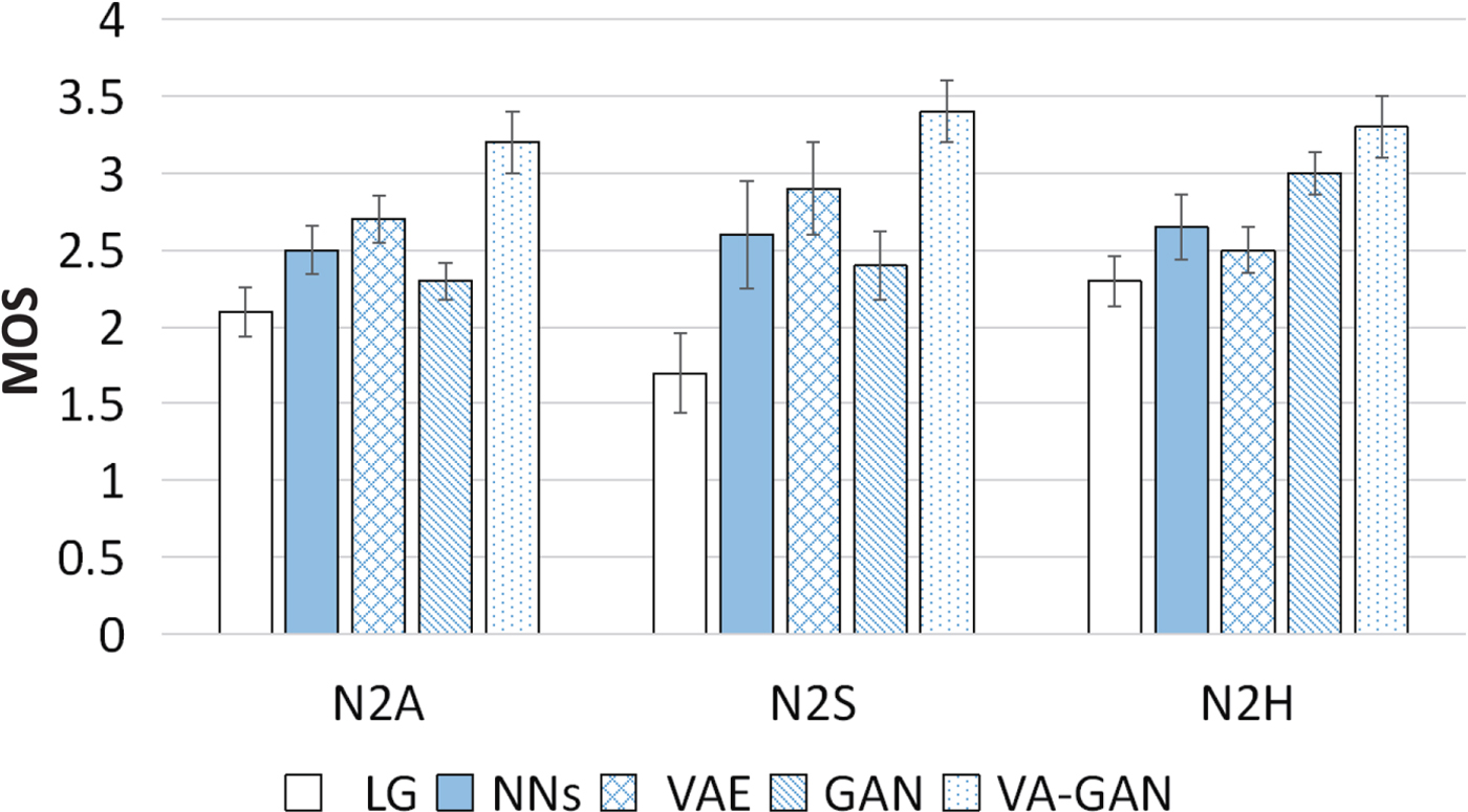
Fig. 9. MOS evaluation of emotional voice conversion.
For the similarity evaluation, we carry out a subjective emotion classification test for neutral to emotional pairs (N2H, N2S, N2A) comparing different methods (LG, NN, GANs, VA-GAN). For each test model, 30 utterances (10 for angry, 10 for sad, 10 for happy) are selected, and 10 listeners are involved. The listeners are asked to label a converted voice as Angry (Ang), Sad, Happy (Hap) or Neutral (Neu). As shown in Table 3 (a), when evaluating the original recorded emotional speech utterances, the classifier performed quite strongly; thus, the corpus is sufficient for recognizing emotion.
Table 2. Table 2. Details of network architectures of Enc, C and D

Table 3. Results of emotion classification for recorded (original) voices and converted voice by different methods [%]

As shown in Table 3 (b), the conventional LG method shows poor performance in all emotional VC tasks. Comparing the results of Table 3 (c) and Table 3 (d), it is clear that NNs method obtains better classification results than the GANs model. With reference to the results of VA-GAN shown in Table 3 (e), the proposed method yielded about 70% classification accuracy on average, which has indicated a significant improvement over the other models.
V. CONCLUSIONS
In this paper, we propose an effective neutral-to-emotional VC model, using the training model VA-GAN, which consists of two effective generator models (GAN and VAE). For the feature extraction and processing, we use CWT to systematically capture the F0 features of different temporal scales (CWT-F0 features), which are suitable for the VA-GAN model. Moreover, to increase the training data for the emotional VC, we carry out the cross-wavelet transforming for CWT-F0 features of different emotional voices to get the XWT-F0 features. A comparison between the proposed VA-GAN and conventional methods shows that our proposed model can effectively change the voice prosody better than other models, and adding the XWT-F0 features can improve the training effectiveness of the training model.
FINANCIAL SUPPORT
This work was supported in part by PRESTO, JST (Grant No. JPMJPR15D2).
Zhaojie Luo was born in Fujian, China, in 1989. He received his M.E.degree from Kobe University in Japan. He is currently a Ph.D. student in computer science at the same university. His research interest is voice conversion, facial expression recognition, multimodal emotion recognition and statistical signal processing. He is a member of IEEE, ISCA and ASJ. He has published more than 10 publications in major journals and international conferences, such as IEEE Trans. Multimedia, EURASIP JASMP, EURASIP JIVP, INTERSPEECH, SSW, ICME, ICPR, etc.
Jinhui Chen received his Ph.D degrees at Kobe University, Japan, in 2016. He is currently an assistant professor at Kobe University. His research interests include pattern recognition and machine learning. He is a member of IEEE, ACM, and IEICE. He has published more than 20 publications in major journals and international conferences, such as IEEE Trans. Multimedia, EURASIP JIVP, SIViP, ACM MM, ACM ICMR, etc.
Tetsuya Takiguchi received the M. Eng. and Dr. Eng. degrees in information science from Nara Institute of Science and Technology, Japan, in 1996 and 1999, respectively. From 1999 to 2004, he was a Researcher in IBM Research, Tokyo Research Laboratory. From 2004 to 2016, he was an associate professor at Kobe University. Since 2016 he has been a professor at Kobe University. From May 2008 to September 2008, he was a visiting scholar at the Department of Electrical Engineering, University of Washington. From March 2010 to September 2010, he was a visiting scholar at the Institute for Learning & Brain Sciences, University of Washington. From April 2013 to October 2013, he was a visiting scholar at the Laboratoire d'InfoRmatique en Image et Systèmes d'information, INSA Lyon. His research interests include speech, image, and brain processing, and multimodal assistive technologies for people with articulation disorders. He is a member of the Information Processing Society of Japan and the Acoustical Society of Japan.
Yasuo Ariki received his B.E., M.E., and Ph.D. in information science from Kyoto University in 1974, 1976, and 1979, respectively. He was an assistant professor at Kyoto University from 1980 to 1990, and stayed at Edinburgh University as visiting academic from 1987 to 1990. From 1990 to 1992 he was an associate professor and from 1992 to 2003 a professor at Ryukoku University. From 2003 to 2016, he was a professor at Kobe University. He is mainly engaged in speech and image recognition and interested in information retrieval and database. He is a member of IEEE, IEICE, IPSJ, JSAI, and ASJ.


 Open access