
I. INTRODUCTION
During the past decades, a tremendous improvement of video coding algorithms has been observed. In January 2013, the Joint Collaborative Team on Video Coding (JCT-VC) of ITU-T VCEG and ISO/IEC MPEG finished the technical work for the latest video coding standard, High-Efficiency Video Coding (HEVC) [1,Reference Wien2], which is also referred to as H.265 by ITU-T and as MPEG-H Part 2 by ISO/IEC. For the same visual quality, depending on the selected configuration and application, HEVC enables a bit rate reduction of 40–60% compared with the predecessor standard Advanced Video Coding (AVC) [Reference Hanhart, Rerabek, De Simone and Ebrahimi3,Reference De Cock, Mavlankar, Moorthy, Aaron and Tescher4]. After the finalization of HEVC, the research for new coding tools is stimulated by a constant strive for even higher coding efficiency [Reference Laude, Adhisantoso, Voges, Munderloh and Ostermann5].
The prediction tools, which led to the prosperous application of these video coding standards, can be roughly distinguished into inter and intra coding tools. In contrast to intra coding, which solely employs spatial redundancy in the current picture, inter coding additionally uses motion compensated prediction to reduce the temporal redundancy between subsequent pictures to further increase the coding efficiency. For typical video signals, the resulting bit rates to achieve the same visual quality are, therefore, for intra coding considerably higher (10–100 times) compared with inter coding.
Nevertheless, intra coding is an essential part of all video coding applications and algorithms: it is used to start transmissions, for random access (RA) into ongoing transmissions, for error concealment, in streaming applications for bit rate adaptivity in case of channels with varying capacity, and for the coding of newly appearing content in the currently coded picture. Additionally, intra coding algorithms are predestined for efficient still image coding. This can be considered as a special case of a video sequence with just one picture. For example, the High-Efficiency Image File Format as a container for HEVC encoded pictures is used as the default image file format on mobile devices running iOS which were released since 2017.
The intra prediction as specified by the HEVC standard is based on the spatial prediction of sample valuesFootnote 1 based on neighboring, previously coded sample values (reference values) followed by a transform coding of the prediction error [Reference Lainema, Bossen, Han, Min and Ugur6]. For the prediction, there are 33 directional modes, one mode for the planar prediction, and one mode for the prediction with the mean value of the reference values (DC mode). The reference values are located in a 1 pel wide column and a 1 pel high row of sample values within previously coded blocks directly to the left and top of the currently coded block (reference area). The directional modes allow for the linear extrapolation of the reference values in the direction of 33 different angles. Considering that there are many horizontal and vertical structures in typical video sequences, a higher angle resolution is selected for these directions [Reference Min, Lee, Kim, Han, Lainema and Ugur7]. The directional modes aim at the prediction of blocks with the linear structure or linear contours [Reference Lainema, Bossen, Han, Min and Ugur6]. Not all blocks to be coded comprise a linear structure. For blocks without a linear structure, the prediction with the DC mode and with the planar mode (weighted combination of four sample values) were developed [Reference Lainema, Bossen, Han, Min and Ugur6].
An analysis of the intra coding in the HEVC standard reveals multiple limitations:
(i) The reference area is relatively small with a width or height of 1 pel, respectively. Further information could be gained by processing additional neighboring, previously coded sample values.
(ii) The directional modes only enable the prediction of linear structures.
(iii) In the case of directional prediction, only one direction per block can be selected by encoders.
In consequence, blocks with non-linear contours or with multiple contours in different directions are difficult to predict. This conclusion is in line with the finding of Lottermann and Steinbach in their work on signal-dependent bit rate modeling [Reference Lottermann and Steinbach8]. Their finding (high bit rates for blocks with many edges) matches our premise that blocks with many edges are difficult to predict.
To overcome these limitations, we propose Contour-based Multidirectional Intra Coding (CoMIC). The underlying principle of the CoMIC prediction is the detection and modeling of contours in already reconstructed blocks followed by the extrapolation of the contours into the currently coded block. Namely, the main contributions of this paper are:
(i) four non-linear contour models,
(ii) an algorithm for the connection of intersecting contours,
(iii) an along-edge sample value continuation algorithm,
(iv) and a mode decision algorithm for the selection of the best contour model based on the Boundary Recall.
The remainder of this paper is organized as follows: In Section II, we discuss related work from the literature and elaborate on the distinguishing features of our work. In Section III, we start by introducing the CoMIC framework, present our novel non-linear contour modeling and extrapolation algorithms, our sample value prediction algorithm, our mode decision algorithm, and our codec integration. Subsequently, in Section IV, we evaluate our algorithms and demonstrate their efficiency by comparing them with the closest works from the literature.
II. RELATED WORK
The findings of numerous works in the academic literature indicate that valuable information for the prediction of the currently coded block can be extracted from contours in neighboring blocks.
Yuan and Sun demonstrate that a contour map of the currently coded picture is suitable for a fast encoder decision for the selection of a good intra mode [Reference Yuan and Sun9]. In contrast to applying edge information for the sake of an accelerated encoding process, we utilize extracted edge information to increase the coding efficiency with a new coding mode.
Asheri et al. [Reference Asheri, Rabiee, Pourdamghani and Ghanbari10] as well as Au and Chan [Reference Au and Chan11] use contour information for error concealment algorithms. For this purpose, contour information from the current picture (Asheri et al.,) or from the current and the previous picture (Au and Chan) is utilized to conceal transmission errors. Differently, from our approach, their algorithms do not influence the actual coding process but are used as post-processing in case of errors. Furthermore, we assume a causal encoding system in which the reference sample values can only be in previously coded blocks.
Liu et al., increase the coding efficiency of JPEG (in [Reference Liu, Sun, Wu, Li and Zhang12]) and of JPEG 2000 as well as AVC (in [Reference Liu, Sun, Wu and Zhang13,Reference Liu, Sun and Wu14]) with contour-based inpainting and texture synthesis algorithms. Their algorithms include the signaling of contour shapes similar to JBIG, the linear extrapolation of contours from already coded parts of the picture, the signaling of patches for texture synthesis, the signaling of representative sample values for the inpainting, and the solving of partial differential equations for the inpainting. In contrast to the HEVC intra coding algorithm, this enables the prediction of multiple contours with different directions per block. Liu et al., achieve an increased coding efficiency. However, only linear contours are extrapolated. Moreover, for the sample value prediction it is required to either signal a considerable amount of side information (patches for texture synthesis) or to solve computationally complex systems of partial differential equations for the inpainting (the decoding of a picture with 512 × 512 pel spatial resolution takes “multiple minutes” [Reference Liu, Sun and Wu14]). Considering that the coding efficiency of their algorithm is only demonstrated for solely intra-coded pictures (all-intra) [Reference Liu, Sun, Wu and Zhang13,Reference Liu, Sun and Wu14], it cannot be assumed that the visually pleasing results of the texture synthesis are a good prediction for subsequently coded pictures.
To compensate for the described limitations of the algorithm of Liu et al., we proposed CoMIC in our conference paper [Reference Laude and Ostermann15] to increase the coding efficiency of JPEG and HEVC. In general, JPEG coding is extended by a spatial prediction and the DCT is computed on the prediction error instead of the signal to be coded. By combining a prediction with the coding of the prediction error, the problem of Liu et al., that the synthesized picture is unsuitable as a prediction reference is circumvented. Like the approach of Liu et al., this first version of CoMIC (v1) is based on the separate processing of contours and sample value prediction. The contours are detected in the reference area (which is three times the size of the currently coded block) and extrapolated linearly into the currently coded block without the signaling of any side information. The sample value prediction is based on the continuation of neighboring sample values along the extrapolated contours. In contrast to the sample value prediction as specified by the HEVC standard, the individual contours are treated separately in our approach. This way, the sample values can be continued in multiple directions per block.
CoMIC v1 is suitable for the prediction of linear contours and structures. However, in real images and video sequences, there are plenty of non-linear contours which cannot be predicted by CoMIC v1. As a consequence of this limitation, CoMIC v1 allows a reliable prediction only in those areas of the currently coded block which are in proximity to the reference area. The contour extrapolation with this algorithm into parts of the block which are further away from the reference area results in a too large uncertainty with respect to the contour shape. In turn, this results in a high prediction error and a high bit rate to compensate for this prediction error. Hence, a distance-dependent diminishing of the continued reference sample value to the mean value of all reference samples is applied [Reference Laude and Ostermann15].
In our experimental section, our novel non-linear CoMIC algorithm (CoMIC v2) will be compared with the algorithm of Liu et al., and to the first version of CoMIC from our conference paper.
The main difference between our contribution and related inpainting approaches is that we assume a causal encoding system where only already coded blocks (i.e. above of and to the left of the current block) are available for the contour extrapolation. In contrast to that, inpainting approaches use the signal on all sides of the missing block. For example, Liu et al., signal the sample values on the contours in the currently coded block as side information and construct Dirichlet boundary conditions this way in their respective method. This knowledge is highly beneficial for the prediction. Taking into account that this information is not available for the decoder without signaling, our method solves a harder problem and also requires less signaling overhead. A proof-of-concept for PDE-based video compression is demonstrated by Andris et al. [Reference Andris, Peter and Weickert16].
In the work [Reference Rares, Reinders and Biemond17], Rares et al., proposed a method for image restoration (i.e. artifact removal). There are multiple commonalities between the related work and our paper: The starting point in both works is similar. Some content is missing, in our case because a block is to be predicted, in the case of Rares et al., because the content is occluded by an artifact. Then, the aim in both works is to “invent” the missing content. In our case by prediction, in the case of Rares et al., by restoration. Additionally, both works are based on contours. Their work is based on modeling the connection of “strongly related” contours on opposing sides of the artifact. The knowledge of where contours end at the other side of the unknown area is highly beneficial for reconstructing the contour in the unknown area. Unfortunately, this knowledge is not available in a causal coding system where blocks are encoded one after another. In consequence, the model proposed by Rares et al., is not transferable to the prediction problem in a causal coding system.
III. CONTOUR-BASED MULTIDIRECTIONAL INTRA CODING
In this section, we discuss the novel contributions of this paper. For the sake of a cohesive presentation, we start by reviewing the CoMIC framework briefly. Subsequently, we elaborate on our novel non-linear contour modeling and extrapolation algorithms, our sample value prediction algorithm, our mode decision algorithm, and describe the integration of the above mentioned algorithms in the CoMIC codec.
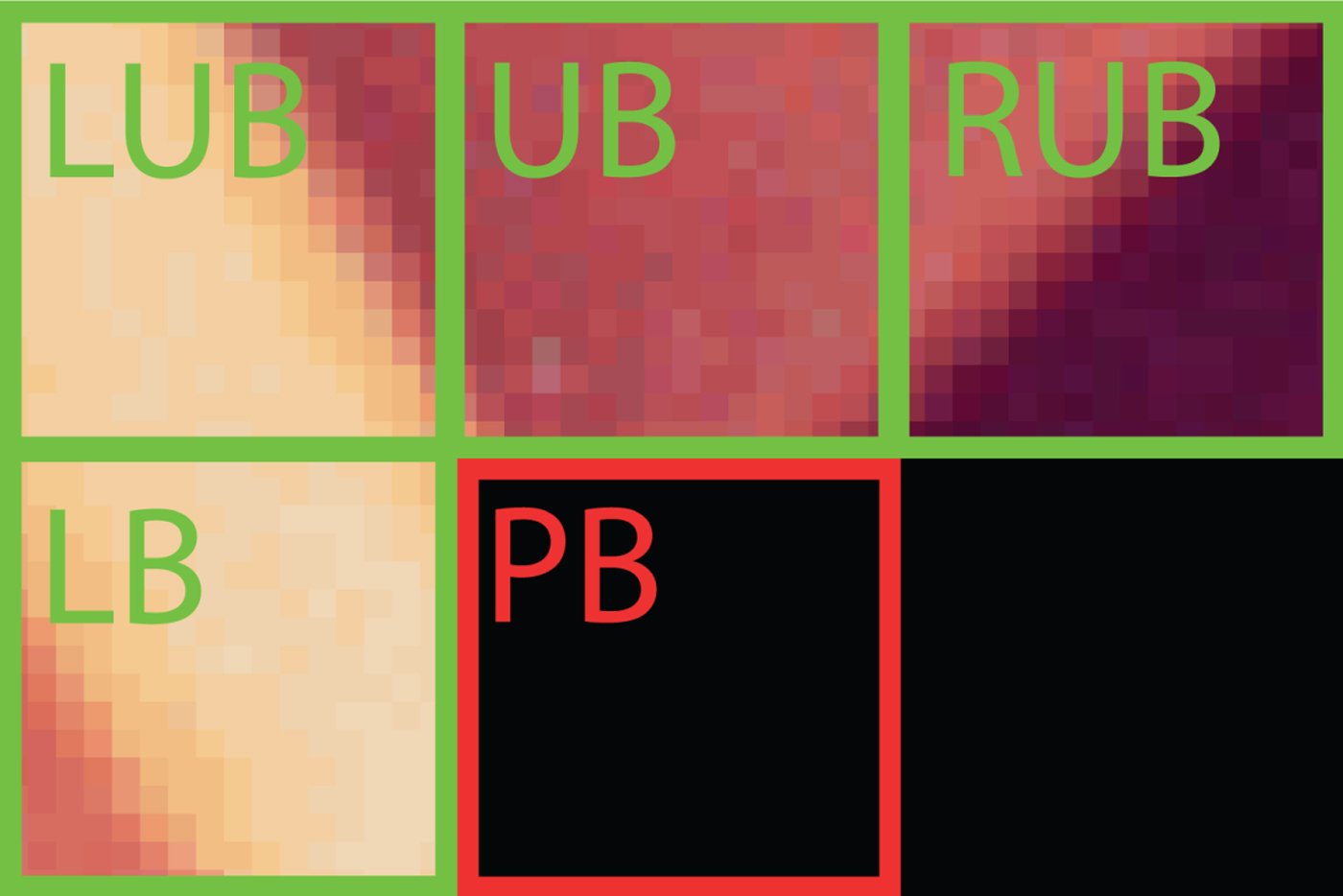
With CoMIC, we designed an intra coding mode for the prediction in multiple directions with minor signaling overhead by combining contour detection, contour parameterization, and contour extrapolation algorithms with conventional video coding algorithms like sample value continuation. As a basic working principle, contour information is extracted from reconstructed samples and employed to extrapolate these contours into the currently coded block. In this pipeline, we limit our area of operation to the currently coded block and the adjacent blocks as illustrated in Fig. 1. The blocks in the reference are of the same size as the currently coded block.
Area of operation. For the prediction of the current block (predicted block, PB), the following four blocks highlighted by green boundaries are used as reference: left block (LB), left-upper block (LUB), upper block (UB), and right-upper block (RUB). In this example the block size is 16×16.
A) CoMIC framework
Both versions of the CoMIC codec (v1 published as [Reference Laude and Ostermann15], v2 proposed in this paper) share the same basic working principle which will be discussed with reference to Fig. 2.
CoMIC v1 pipeline: the contours are detected using the Canny algorithm, labeled, modeled with linear functions, and extrapolated into the currently coded block. The major limitation of CoMIC v1 is the linear contour model. In consequence, the contours can only be extrapolated partly into the currently coded block because the accuracy of the extrapolated contours drops considerably with increasing distance from the reconstructed area. (a) Detected contours, (b) Labeled contours, (c) Modeled contours, (d) Extrapolated contours.
The encoding of a block starts by detecting contours in the reference area (see Fig 2a). Our contour detection is based on the well-known Canny edge detection algorithm [Reference Canny18]. A minor additional coding gain (0.3%) can be achieved by using more advanced edge detection algorithms like [Reference Dollar and Zitnick19], but this also increases the computational complexity by a factor of 90 for the entire encoder. Thus, we chose to content ourselves with the original Canny edge detector for this paper.
Once the edges have been detected with the Canny algorithm, a binary image is available that describes all edge pixels in the reconstructed area. Our goal is the extrapolation of distinctive contours. Therefore, we label individual contours in the binary edge picture with the algorithm of Suzuki and Abe [Reference Suzuki and Abe20] (see Fig 2b).
The part of the framework as it is described so far is maintained for this paper. In the following, we briefly present the remainder of the framework as it was used for our conference paper. It is noteworthy that the following parts of the framework will not be used by the contributions of this paper but are described for the sake of cohesiveness.
In [Reference Laude and Ostermann15], each contour is modeled by a straight line (see Fig 2c), i.e. by a polynomial parameterization with two parameters. For contours which hit the left border of the currently coded block, the horizontal coordinate x is used as the independent variable while the vertical coordinate y is used as the independent variable for contours that hit the upper border of the currently coded block. This differentiation facilitates the parameterization of horizontal and vertical structures. Thus, the polynomial p(a), with a being the independent variable (i.e. either x or y) and with coefficients  $\beta _i\in {\open R}$ is parameterized as noted in equation (1):
 $$p(a) = \beta_0 + \beta_1 a. $$
The coefficients βi are determined by minimizing the mean squared error between the detected contour and the linear contour model using a least squares regression.
With the parameterization of the contour available, the contour can be extrapolated in the currently coded block. As disclosed in Section II, our linear contour model only allows an accurate extrapolation in parts of the currently coded block (see Fig 2d). The reference sample values are continued parallel to the linearly extrapolated contours to predict the sample values of the current block. In the course of the continuation, the sample values are diminished towards the mean value of the reference sample values due to the discussed limitation of the linear contour model. As a fallback solution for blocks without extrapolatable contours, a DC mode similar to the DC mode as specified by the HEVC standard is available.
B) Non-linear contour modeling
As it was revealed in the previous sections, the major limitation of CoMIC v1 is the lack of capability to model non-linear contours. To overcome this limitation, we propose four different non-linear contour models in this paper. A Boundary Recall-based contour model selection algorithm is applied to select the best model for each block.
Naturally, the straightforward extension of our linear contour model towards a non-linear model is a polynomial model with three or more parameters. Thus, as first non-linear contour model, we propose a quadratic function. Extending equation (1), the model is formulated as in equation (2):
 $$p(a) = \beta_0 + \beta_1 a + \beta_2 a^2,$$
This model will be referred to as Contour Model 1. Similarly to the linear model, the independent variable is chosen depending on whether the contour enters the predicted block horizontally (x is the independent variable) or vertically (y is the independent variable). In the following, we describe the polynomial calculation only for x as an independent variable. For n given edge pixels (x i, y i) with i=1, …, n we write equation (3):
 $$ {\bf x}= \left[\matrix{x_1 \cr \vdots \cr x_n} \right] \in {\open R}^{n \times 1}, \quad {\bf y}= \left[\matrix{y_1 \cr \vdots \cr y_n}\right] \in {\open R}^{n \times 1}.$$
The approximation of the contour is written as in equation (4) with ε as approximation error:
 $$\eqalign{{\bf y} &=\left[\matrix{1 & \cr \vdots & {\bf x} & {\bf x}^2\cr1 &} \right] {\bf \beta} + {\bf \epsilon} \quad \hbox{with } {\bf \beta}= \left(\matrix{\beta_0 \cr \beta_1 \cr \beta_2} \right), {\bf f\epsilon} \in {\open R}^{n\times1}\cr &= {\bf X} {\bf \beta} + {\bf \epsilon}.}$$
This linear regression problem (with βi as regression parameters) can be solved with a least squares approach, i.e. by minimizing f(β) in equation (5):
 $$f({\bf \beta})=({\bf y} - {\bf X \beta})^T({\bf y} - {\bf X \beta})$$
The estimated regression parameters, denoted as  $\hat{\bf \beta}$, are calculated as in equation (6):
 $$\hat{\bf \beta} = ({\bf X}^T {\bf X})^{-1} {\bf X}^T {\bf y}.$$
This model enables a favorable approximation for some contours. However, we observed that this model is not robust enough for all contours by reason of the small number of contour pixels (on which the regression is performed) and that to some extend imprecise contour location and volatile contour slope. Considering these reasons, we project the contour information into a different space prior to the modeling for the remaining three contour models. To be precise, we model the curvature of the contour by modeling the slope of the contour location linearly. This model is more robust than the quadratic model since it has fewer parameters. Additionally, the slope is smoothed to reduce the volatility of the curvature.
Let m i denote the slope of the contour at location i. Furthermore, let
 $${\bf m}= \left[\matrix{m_1 \cr \vdots \cr m_n} \right] \in {\open R}^{n \times 1},$$
with
 $$m_i = {y_{i+1} - y_i \over x_{i+1} - x_i}.$$
Note that the denominator could be zero if no precautions were taken. This is due to the fact that the contour location is only determined with full-pel precision. The difference of the independent variable for two neighboring contour pixels is calculated in the denominator. Therefore, the problem arises in cases when two neighboring contour pixels share the same value for the independent variable (e.g. for narrow bends). To circumvent the problem, a single value of the dependent variable is interpolated from the two values of the neighboring pixels. Thereby, only one slope value (instead of two) needs to be calculated for this value of the independent variable. No difference of the independent variable needs to be computed if two pixels share the same value for this variable as these two pixels are combined to one data point. Then, the second non-linear contour model which we refer to as Contour Model 2 is formulated as in equation (7):
 $$\eqalign{{\bf m} &= \left[\matrix{1 & \cr \vdots & {\bf x} \cr 1 &} \right] {\bf \gamma} + {\bf \epsilon} \quad {\rm with} {\bf \gamma} = \left(\matrix{\gamma_0 \cr \gamma_1} \right), {\bf \epsilon} \in {\open R}^{n \times 1} \cr &= {\bf M \gamma} + {\bf \epsilon},}$$
where γ describes the regression coefficients which can be approximated by applying equation (9) analogously.
It is known that it can be beneficial to address outliers when formulating approximation models. Therefore, adopting the approach of Holland and Welsch [Reference Holland and Welsch21] to iteratively reweighten the least squares residues, we propose the third contour model (Contour Model 3). The weights ωi for the residues r i are calculated with an exponential function which is parameterized by the largest residue (r max) as noted in equation (8):
 $$\omega_i = e^{-({2r_i}/{r_{{\rm max}}})^2}.$$
Given the weights from one iteration, the regression parameters for the next iteration can be calculated by reformulating equation (6) to:
 $$\hat{\bf \gamma} = ({\bf M}^T {\bf WM})^{-1}{\bf M}^T{\bf Wm},$$
with
 $${\bf W} = \left(\matrix{\omega_1 &0 & \cdots & 0 \cr 0 & \omega_2 & \cdots & 0 \cr \vdots & \vdots & \ddots & \vdots \cr 0 & 0 & \cdots & \omega_n} \right),$$
where  $\hat{\bf \gamma}$ is the estimation of the regression parameters γ. The actual number of reweighting iterations is not of crucial importance for the regression result as long as the number is sufficiently high. Hence, it is chosen as 15 since the computational complexity is negligible as evaluated in Section IV.
None of the three proposed non-linear contour models considers that the curvature of the contour may change unexpectedly – i.e. evasive by equation (7) – in the reference area. As means against such evasive contour changes in the reference area, we propose a fourth contour model (Contour Model 4). The rational for this model is that in cases of such contours, it is undesirable to consider parts of the contour which are far away from the currently coded block. Thus, the residues for the regression are weighted depending on their distance to the currently coded block. To be precise, the weights decrease linearly with increasing distance. In contrast to Contour Model 3, the regression is only performed once for Contour Model 4 since the distance does not depend on the weights.
It is worth mentioning that it became apparent in our research that splines – although being often used for signal interpolation – are not capable of achieving a good contour extrapolation. Moreover, our research revealed that higher order polynomial models (i.e. cubic and higher) are not robust enough.
C) Contour extrapolation
With the contour modeling being accomplished by the four proposed models from Section III.B, the extrapolation of the contours which are modeled will now be described.
For Contour Model 1, the contour is extrapolated by directly calculating new function values with equation (2) for the independent variable in the predicted block. For the other three models which model the slope of the contour, the extrapolation is performed analogously by respectively derived equations.
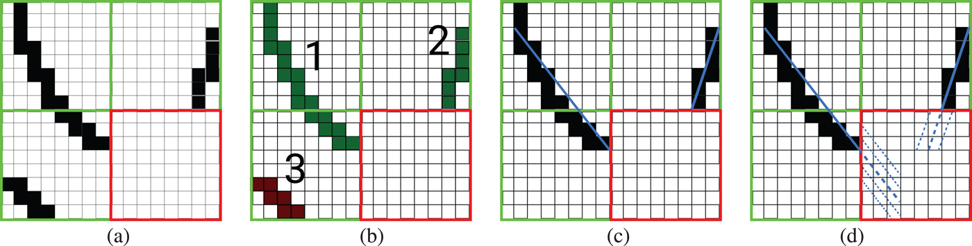
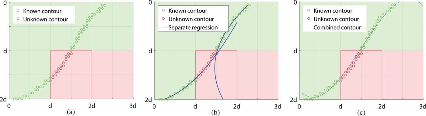
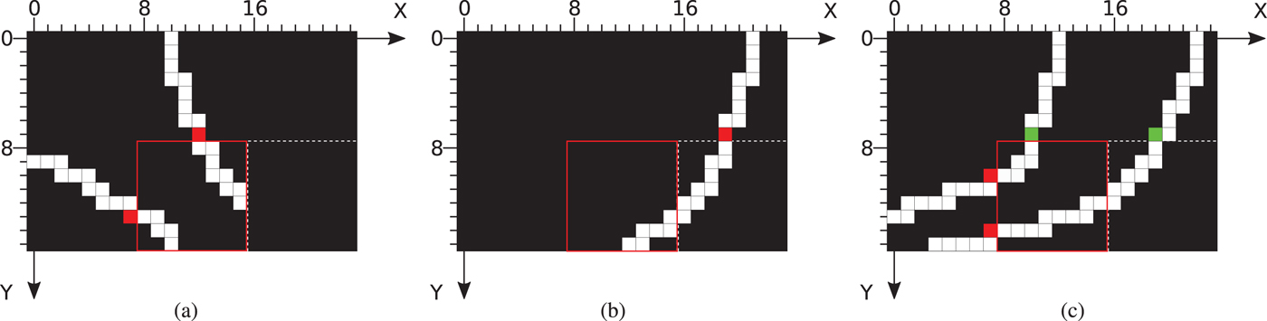
This extrapolation algorithm works reliably in most cases. However, it may fail for contours which start in the reference area, proceed through the predicted block, and reenter the reference area. An example of such a contour is illustrated in Fig. 3a. For the contour modeling, it appears as if there are two independent contours in the reference area. The independent extrapolation of these two contours is shown in Fig. 3b. Although the extrapolation of one contour is accurate with respect to the original contour, the extrapolation of the second contour would cause a considerable prediction error. As a solution to this issue, it is detected that these two contours form one contour and they are processed together. For this purpose, the contour points of the two to-be-combined contours are summarized to one contour at first. Then, the contour pixels of this combined contour are modeled using the same independent variable. For this combined contour, considering that a section in the middle of the contour is to be predicted, the extrapolation problem turns into an interpolation problem which is approached with a cubic polynomial regression as illustrated in Fig. 3c.
Combination of intersecting contour parts. (a) Original contour shape, (b) Separate extrapolation of the two contour parts results in inaccurate prediction, (c) Combination of the two contour parts and transfer of the extrapolation problem into an interpolation problem results in accurate prediction.
D) Sample value prediction
With the contours extrapolated following the description in Section III.C, the sample values can be predicted by utilizing the extrapolated contours. The sample value prediction is based on the continuation of boundary sample values. Three cases can be distinguished. They are discussed following the illustration in Fig. 4.
Different cases for the sample value prediction along the contours. (a) Contours hit the predicted block directly, (b) Contour hits the predicted block indirectly, (c) Combination of contours.
In the first case as illustrated in Fig. 4a, the contours directly hit the predicted block either from the top or from the left. In this case, the sample value of the contour pixel directly adjacent to the predicted block (highlighted in red) is used as a reference and extrapolated along the contour. Slightly different is the second case (Fig 4b) in which the contour hits the predicted block indirectly via the neighboring block on the right side. Here, the sample value of the adjacent pixel on the right side of the predicted block is unavailable as a reference since this pixel is not yet predicted. Hence, the sample value of the nearest available reference pixel (which is highlighted in red) from the top-right block is used as reference. As for the first case, this reference sample is continued along the contour. The commonality of these two cases is that the reference sample value is continued unaltered. This is different in the third case which is used for combined contours as shown in Fig. 4c: For such contours, there are two reference sample values, one at each end of the extrapolated contour. Since these two reference sample values may be different, we chose to linearly blend the predicted sample values between them.
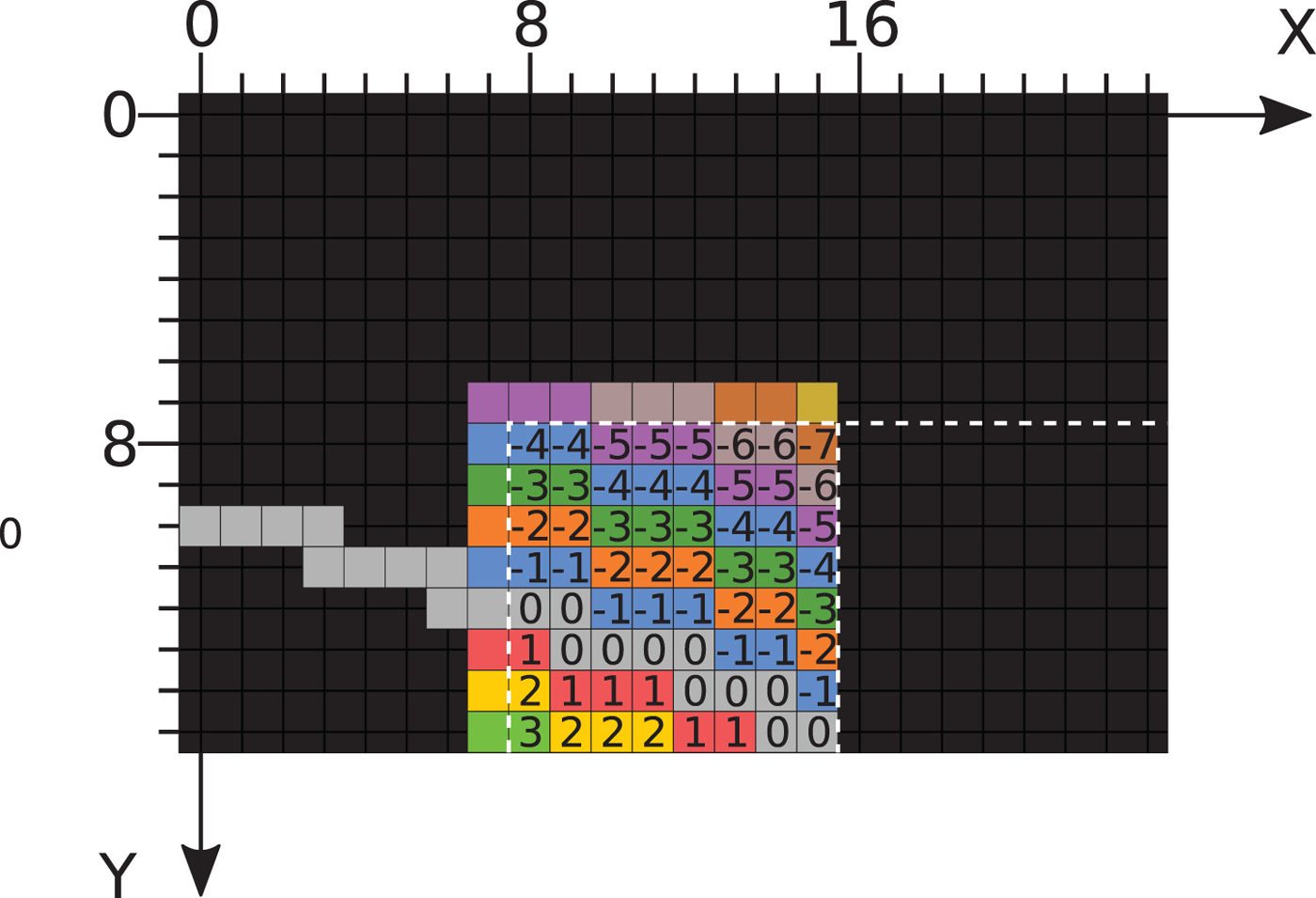
So far, only the sample values on the contour are predicted. To predict the remaining sample values, the above-described process is extended horizontally or vertically, depending on the orientation of the contour. The reference sample values whose pixel location has an offset to the hit point between contour and block boundary in horizontal or vertical direction, respectively, are continued parallel to the extrapolated contour. An example is illustrated in Fig. 5. Here, the numbers indicate the offset of the location of the reference pixels.
Illustration of the sample value prediction. The numbers indicate the offset of the location of the reference pixel with respect to the reference pixel on the contour.
In the presence of multiple contours, the predicted sample value of a non-contour pixel can be obtained from multiple references. One of our premises is that contours are located at the borders of objects. Therefore, sample values are continued up to the next contour. Individual contours are processed in a clockwise direction.
Our decision to base the sample value prediction on the continuation of neighboring reference sample values is backed up by multiple reasons: (1) The continuation of the reference sample is well understood from the intra coding algorithms in recent video coding standards [Reference Lainema, Bossen, Han, Min and Ugur6,Reference Ostermann22]. (2) In contrast to inpainting algorithms, the complexity is moderate (cf. Section IV). (3) In contrast to texture synthesis algorithms, the reconstructed signal (i.e. the sum of the predicted signal and the transmitted quantized prediction error) is suitable as a reference for future predictions.
E) Contour model selection
In total, there are four non-linear contour models. One of them needs to be selected per block by the encoder. The premise of our work is that it is beneficial to process structural information (i.e. contours) and textural information (i.e. sample values) separately. Hence, the decision for the best contour model cannot be based on the quality of the predicted sample values (e.g. by measuring the MSE). Instead, the decision is based on the accuracy of the extrapolated contours. As the original contours are known at the encoder, the extrapolated contours can be compared with the original contours.
The Boundary Recall [Reference Ren and Malik23] is chosen as a metric to measure the accuracy of the extrapolated contours. This metric is commonly used to measure the accuracy of superpixel boundaries [Reference Achanta, Shaji, Smith, Lucchi, Fua and Süsstrunk24,Reference Reso, Jachalsky, Rosenhahn and Ostermann25]. Since these two tasks (measuring the accuracy of extrapolated contours and superpixel boundaries, respectively) are very similar, we believe that the BR is a suitable metric for our case. Letting n orig, n ext, and n mutual denote the number of pixels of the original contour, the number of pixels of the extrapolated contour, and the number of pixels which are mutual for the original and the extrapolated contour, respectively. Then, the BR is defined as in equation (11):
 $${\rm BR} = \left\{\matrix{\displaystyle{n^{2}_{\rm mutual} \over n_{\rm orig} \cdot n_{\rm ext}} \hfill &\hbox{for}\, n_{\rm orig} \gt 0, n_{\rm ext} \gt 0 \hfill \cr 0 \hfill &{\rm otherwise}. \hfill}\right.$$
The same contour model is selected for all contours in the predicted block. It is worth noting that different models might be better for different contours within the predicted block. Thus, the selection is not optimal. However, the selection of the contour model needs to be signaled to the decoder because the BR cannot be calculated at the decoder due to the absence of the knowledge of the original contour location. Hence, the better trade-off between the selection of a good contour model and signaling overhead is to use only one contour model per block.
F) Codec integration
The proposed algorithms were integrated into the CoMIC stand-alone codec software which was originally proposed in [Reference Laude and Ostermann15]. This new version of the codec is referred to as CoMIC v2.
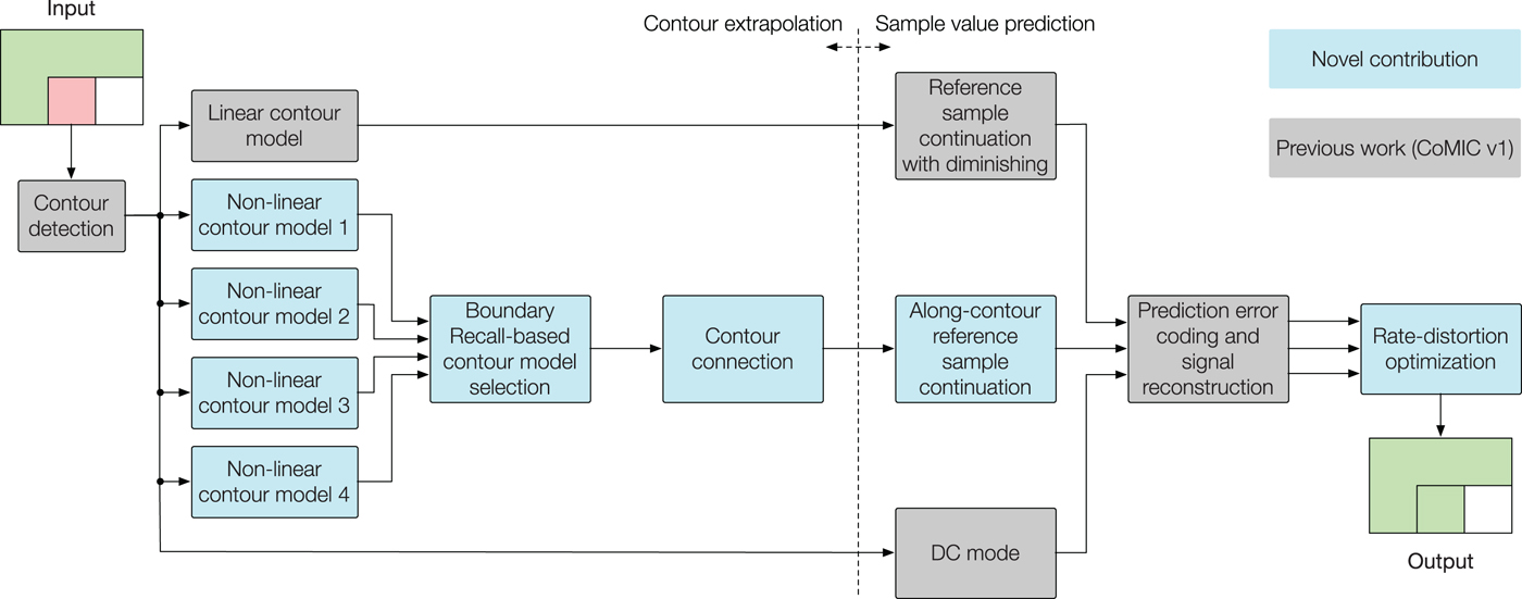
In the following, we will describe the integration of the proposed algorithms in the CoMIC v2 pipeline with reference to Fig. 6. At the encoder, the picture is partitioned into blocks. For the prediction, we use blocks with a size of 32×32. Subsequent to the contour detection, the four different contour models are organized in parallel tracks to the linear contour model. Among the four non-linearly extrapolated contours, the most accurate extrapolation is chosen with the Boundary Recall-based contour model selection. In the case of intersecting contours, the contour connection algorithm is applied. Thereby, the contour extrapolation is finished. Consecutively, the sample values are predicted along the non-linearly extrapolated contour. After this stage, there are three predicted signals: one for the linear prediction, one for the non-linear prediction, and as fall-back one for the DC mode. For these three predicted signals, the prediction error is transform coded (DCT and quantization) and the signal is reconstructed with the quantized prediction error. It is worth noting that we use a different block size for the encoding of the prediction error than for the prediction, namely the same 8×8 block size which is used for JPEG. The reason is that this allows to measure the gain of our prediction over the direct encoding of the picture as it is done by JPEG. For the same reason, we utilize the same quantization matrix which is suggested by the Independent JPEG Group and implemented in the JPEG reference software [26].
CoMIC v2 pipeline. Novel contributions of this manuscript are in blue blocks, contributions from our previous work [Reference Laude and Ostermann15] are in gray blocks.
Finally, the best mode is selected by a rate-distortion optimization [Reference Sullivan and Wiegand27]. The selection of a Lagrange multiplier for rate-distortion optimization is non-trivial. This states true especially since the rate-distortion optimization is an application-specific task. Hence, there is no single correct λ value. Basically, choosing a Lagrange multiplier is about expressing how the distortion would change in case of a slightly changing bit rate. Therefore, we modeled this change as a function of the quality parameter for the MSE(rate) curve for the picture Milk.
IV. EVALUATION
In this section, we will describe the experiments we performed to evaluate the proposed methods. In [Reference Laude and Ostermann15], we integrated our algorithm into the HEVC reference implementation (HM) and proposed a stand-alone codec implementation to enable a comparison with related works from the literature. Similarly, for this paper, we implemented the proposed algorithms into the stand-alone CoMIC software and into HM as well.
Liu et al., chose to measure the performance of their method in terms of bit rate savings over JPEG at a JPEG quality of 75. In [Reference Laude and Ostermann15], we adopted this procedure. We do the same for this paper to compare the performance of our new contour models with these two related works. The resulting bit rate savings are listed in Table 1Footnote 2. It is worth noting that only a limited number of test pictures were used in [Reference Liu, Sun, Wu, Li and Zhang12]. The subset is highlighted by a star (*). For this paper, we extend the set of used pictures to all pictures listed in the table. However, to facilitate an overview at a glance, we calculate a separate average value for the *-subset. CoMIC v2 achieves bit rate savings between 23.6% and 37.4% over JPEG. In average, 30.9% (and 32.6% for the *-subset) are achieved. Thereby, both related works are outperformed. With the new contribution proposed in this paper and incorporated in CoMIC v2, the bit rate savings are increased by on average 2.1 percentage points compared with CoMIC v1. Another interesting finding is that the gap over the results of Liu et al., depends on the content in the encoded images. For images with lots of structural parts (e.g. Lena) the gap is larger than for images with many homogeneously colored areas (e.g. Milk or Kodim 02). For the latter, Liu et al., can max out the benefits of their inpainting algorithm.
Bit rate savings over JPEG (quality 75): we compare our algorithm (coMIC v2) with the results from the related work of Liu et al., [Reference Liu, Sun, Wu, Li and Zhang12] and with the results from our conference paper [Reference Laude and Ostermann15]. Both works are outperformed.
The evaluation of bit rate savings for a quality of 75 is a necessary experiment to compare the performance between CoMIC and the related work of Liu et al. In addition to this experiment, we also calculate BD rate [Reference Bjøntegaard28] gains over a wider quality range (30–90) to assess our algorithm for different qualities. BD rate gains indicate bit rate savings for equal PSNR. The results are summarized in Table 2. It is observed that CoMIC v1 and CoMIC v2 achieve BD rate gains of 27.55 and 29.10% over JPEG, respectively. These values are almost the same than those for the bit rates savings at quality 75 (28.8 and 30.9%). It can be concluded that the coding gain is achieved consistently over different qualities. When comparing CoMIC v2 with CoMIC v1, the gain is 2.16%.
BD rate gains over JPEG. Positive values indicate increased coding efficiency. CoMIC v1 is outperformed by CoMIC v2

As second implementation, the proposed algorithms were implemented as additional coding mode in the HEVC reference software HM. The usage of the additional mode is determined by the rate-distortion optimization [Reference Sullivan and Wiegand27] on coding unit level. CoMIC v2 is chosen if it provides the lowest rate-distortion costs. One binary flag for the mode usage is signaled in the bitstream as part of the coding unit syntax. For blocks for which CoMIC v2 is used, an additional syntax element is introduced to indicate the selected contour model. To cover a variety of different contents, 30 test sequences as listed in Table 3 were selected from various databases: MPEG Common Test Conditions [Reference Bossen29] (Steam Locomotive, Kimono, Park Scene, Basketball Drive, BQ Terrace, Johnny), BVI Texture database [Reference Papadopoulos, Zhang, Agrafiotis and Bull30] (Ball Under Water, Bubbles Clear, Calming Water, Carpet Circle Fast, Drops on Water, Flowers 2, Paper Static, Smoke Clear, Sparkler, Squirrel) and action camera content [Reference Laude, Meuel, Liu and Ostermann31] (Bike). The encoder was configured in all the intra, RA, and low delay configurations [Reference Bossen29]. BD rates are calculated following [Reference Bjøntegaard28]. Additionally, as suggested in [Reference Sullivan and Ohm32], weighted average BD rates BDYCbCr were calculated with weighting factors of 6/1/1 for the three color components Y/Cb/Cr. The experimental results are summarized in Table 3. It is observable that HM is noticeably outperformed with BD rate gains of up to 2.48%.
BD rate gains over HM. Positive values indicate increased coding efficieny. It is observed that HM is outperformed.

Some subjective results for the predicted signal are illustrated in Fig. 7. The left column shows the original blocks and the right column shows the corresponding predicted blocks. It can be observed that the non-linear contour are predicted accurately.
Exemplary prediction results for the proposed algorithms. The left column (Sub-figures a, c, e, g) shows the original blocks and the right column (Sub figures b, d, f, h) shows the corresponding predicted blocks.
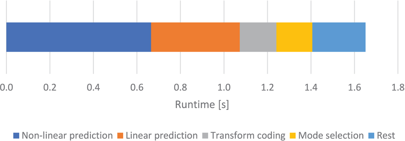
We measure the computational complexity of CoMIC by using the run time on an Intel Core i7-4770 K CPU @ 3.50 GHz as metric. For a 512×512 pel picture (Lena), the encoding requires 1.65 s (excluding the time for file reading and writing). Similar run times are observed for other pictures. Thereby, the CoMIC is very fast compared with the related work from Liu et al., for which the authors indicate a run time of “multiple minutes” for a picture of the same size. A breakdown of this time is illustrated in Fig. 8: The largest part in the run time is caused by the non-linear prediction, followed by the linear prediction, the transform coding, and the mode selection. The decoding time is lower than the encoding time. This is because the encoder tests all modes per block while the decoder only performs the mode which is signaled in the bit stream for a given block.
Run time analysis.
Conceptually, for pictures with linear content, the predictions with CoMIC and with HEVC should be similar. This is demonstrated with the synthetic example in Fig. 9. The most noticeable difference in this example are two blocks that are very close to a contour but next to it. For these blocks the CoMIC DC mode produces a prediction which is slightly too dark. This is caused by the different reference areas for the calculation of the mean sample value in the DC modes of HEVC and CoMIC: While HEVC uses only one row/column of sample values, CoMIC uses the entire reference area as demonstrated in Fig. 1. This is more stable in general, but not for this particular synthetic example in which a contour passes through the otherwise homogeneous reference area. Also, some lines appear to be straighter in case of HEVC. The reason is that for CoMIC v2 they are approximated by a quadratic polynomial whose coefficient for the squared term is not exactly determined as zero by the least-squares estimation. Besides that, this example reveals that CoMIC (which extracts all information from the reconstructed signal) is as good as brute-force selection on block-level of one of 35 HEVC intra prediction modes.
Predicted signals for a synthetic example: it is observable that CoMIC (left) and HEVC (right) can generate a similar prediction for linear structures.
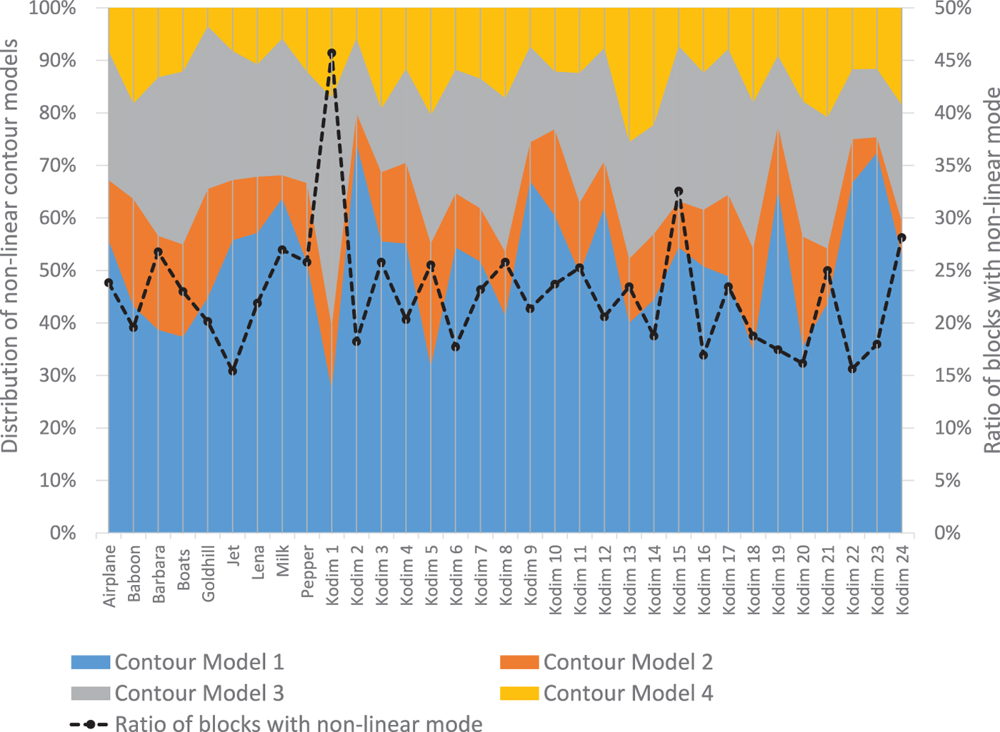
To get a deeper understanding for the four different proposed contour models, we analyze their distribution over the test set. The results are visualized in Fig. 10. On average, in 50.2% Contour Model 1 is selected, in 12.7% Contour Model 2, in 23.8% Contour Model 3, and in 13.3% Contour Model 4. The data also suggest that the modes with small average values have a reason for existence: For some pictures (Fig 11), their share in the distribution is considerably larger than their average values. One example is Kodim 1 for which Contour Model 3 is used more often. This picture shows a brick wall with lots of artifacts in the bricks. The color of the artifacts is similar to the color of the joints. We hypothesize that these artifacts result in outliers after the contour detection, which are subsequently suppressed by the re-weighting of Contour Model 3. Kodim 13 includes wavy water with contours whose slope varies. For such contours the distance-dependent weights of Contour Model 4 are beneficial. This hypothesis is supported by the observation that this contour model is used with an above-average share for this picture. Additionally, the ratio of blocks which are coded using non-linear contour models is illustrated on the right vertical axis of the same figure. Naturally, the number of blocks for which the (non-linear) contour models are applicable is limited by the number of blocks which contain such contours. Our analysis is that the non-linear contour models are primarily used for such blocks.
Distribution of the selected contour models (left vertical axis) and ratio of blocks coded with non-linear contour models (right vertical axis). Contour Model 1 is the regular polynomial model, Contour Model 2 models the slope, Contour Model 3 additionally ensures robustness in case of outliers by iterative reweighting, and Contour Model 4 includes distance-dependent weighting.
Pictures Kodim 1 and Kodim 13.
V. CONCLUSION
In this paper, we proposed non-linear CoMIC. It is based on the following main contributions: four non-linear contour models, an algorithm for the connection of intersecting contours, an along-edge sample value continuation algorithm, and a mode decision algorithm for the selection of the best contour model based on the Boundary Recall. The evaluation reveals that related works are outperformed. Compared with the closest related work, BD rate gains of 2.16% are achieved on average. Furthermore, it is worth noting that the CoMIC method can be integrated into any modern video codec where it could be combined with other beneficial tools like advanced prediction error coding or variable block sizes. Namely, BD rate gains of up to 2.48% were achieved over the HEVC reference implementation HM.
Thorsten Laude Thorsten Laude studied electrical engineering at Leibniz University Hannover with specialization on communication engineering and received his Dipl.-Ing. degree in 2013. In his diploma thesis, he developed a motion blur compensation algorithm for the scalable extension of HEVC. He joined InterDigital for an internship in 2013. At InterDigital, he intensified his research for HEVC. After graduating, he joined Institut für Informationsverarbeitung at Leibniz University Hannover where he currently pursues a Ph.D. He contributed to several standardization meetings for HEVC and its extensions. His current research interests are intra coding for HEVC, still image coding, and machine learning for inter prediction, intra prediction and encoder control.
Jan Tumbrägel Jan Tumbrägel studied electrical engineering at Leibniz University Hannover and received his Dipl.-Ing. degree in 2016.
Marco Munderloh Marco Munderloh achieved his Dipl.-Ing. degree in computer engineering with an emphasis on multimedia information and communication systems from the Technical University of Ilmenau, Germany, in 2004. His diploma thesis at the Fraunhofer Institute for Digital Media Technology dealt with holographic sound reproduction, so-called wave field synthesis (WFS) where he holds a patent. During his work at the Fraunhofer Institute, he was involved in the development of the first WFS-enabled movie theater. At Institut für Informationsverarbeitung of Leibniz University Hannover, Marco Munderloh wrote his thesis with a focus on motion detection in scenes with non-static cameras for aerial surveillance applications and received his Dr.-Ing. degree in 2015.
Jörn Ostermann Jörn Ostermann studied Electrical Engineering and Communications Engineering at University of Hannover and Imperial College London. He received Dipl.-Ing. and Dr.-Ing. from the University of Hannover in 1988 and 1994, respectively. In 1994, he joined AT&T Bell Labs. From 1996 to 2003 he was with AT&T Labs – Research. Since 2003 he is Full Professor and Head of Institut für Informationsverarbeitung at Leibniz University Hannover, Germany. Since 2008, Jörn Ostermann is the Chair of the Requirements Group of MPEG (ISO/IEC JTC1 SC29 WG11). Jörn Ostermann received several international awards and is a Fellow of the IEEE. He published more than 100 research papers and book chapters. He is coauthor of a graduate level text book on video communications. He holds more than 30 patents. His current research interests are video coding and streaming, computer vision, 3D modeling, face animation, and computer–human interfaces.


 Open access