

I. INTRODUCTION
In Japan, 8K 59.94-Hz (60-Hz) satellite video broadcasting (spatial resolution $7680 \times 4320$ ) began December 1, 2018. Meanwhile, the Japanese 8K broadcasting standard (ARIB STD-B32 [1]) also supports a frame-rate of 119.88 Hz (120 Hz), which is twice higher than that of the current 8K broadcasting and facilitates reproducing rapid motion more clearly and smoothly. To verify the effectiveness of high-frame-rate video transmission, we developed the world's first 8K 120-Hz real-time video encoder that complies with the 8K broadcasting standard [Reference Sugito, Iwasaki, Chida, Iguchi, Kanda, Lei, Miyoshi and Uehara2]. The encoder employs the high efficiency video coding (HEVC)/H.265 [3] temporal scalable coding, which is decodable as both 120- and 60-Hz videos from encoded 120-Hz bit-streams, to satisfy the compatibility requirements for 8K 60-Hz broadcasting.
To consider the required bit-rate for 8K 120-Hz temporal scalable video coding for broadcasting purposes, we conducted two types of subjective evaluation experiments using video encoding software that emulates our real-time encoder. In the first experiment, to investigate the required bit-rate for 8K 120-Hz videos, we evaluated videos compressed using four different bit-rates using a general subjective evaluation method for 8K encoded videos. The general method was determined based on an initial 8K subjective evaluation experiment. To the best of our knowledge, particular considerations for 8K subjective evaluation methods, which are mainly caused by the sense of immersion, have never been mentioned, though some papers including 8K subjective evaluation experiments exist (e.g. [Reference Ichigaya and Nishida4,Reference Sugito, Iguchi, Ichigaya, Chida, Sakaida, Shishikui, Sakate, Itui, Motoyama and Sekiguchi5]). Then, based on the first experiment, we compared videos encoded using the same bit-rate to 8K 120-Hz videos and encoded with three different bit-rates to 8K 60-Hz videos to study the appropriate bit-rate for 8K 60-Hz videos within the 8K 120-Hz videos. To assess such slightly different conditions, we employed a new subjective evaluation method for 8K encoded videos. In addition to the considerations on the required bit-rate, we analyzed the encoded videos used for the first experiment to investigate a factor to determine the subjective image quality of our encoder. We further considered experimental settings for future 8K subjective evaluations by analyzing the experimental results.
This paper is a merged version of two conference papers [Reference Sugito, Iwasaki, Chida, Iguchi, Kanda, Lei, Miyoshi and Kazui6,Reference Sugito, Iwasaki, Chida, Iguchi, Kanda, Lei, Miyoshi and Kazui7] and a presentation at an international standardization meeting [Reference Sugito8]. The remainder of this paper is organized as follows. We introduce a general subjective evaluation method for 8K encoded videos in Section 2 and describe the features of the 8K 120-Hz encoder in Section 3. Two informal experiments conducted to study the video bit-rate requirements and the experimental results are provided in Sections 4 and 5. In Section 6, we discuss the required video bit-rate, analyses on encoded videos, and requirements for future 8K subjective evaluations. Conclusions and suggestions for future work are given in Section 7.
II. GENERAL 8K SUBJECTIVE EVALUATION METHOD
This section introduces a general subjective evaluation method for 8K encoded videos based on an initial experiment.
A) Initial 8K subjective evaluation experiment
In 2013, a subjective evaluation experiment was conducted to assess the image quality of the world's first 8K 60-Hz HEVC real-time encoder [Reference Sugito, Iguchi, Ichigaya, Chida, Sakaida, Shishikui, Sakate, Itui, Motoyama and Sekiguchi5]. Tables 1 and 2 show the experimental conditions for the encoder and the viewing conditions for the experiment, respectively.
Table 1. Experimental conditions for 8K 60-Hz HEVC encoder
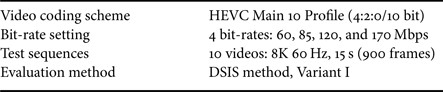
Table 2. Experimental viewing conditions
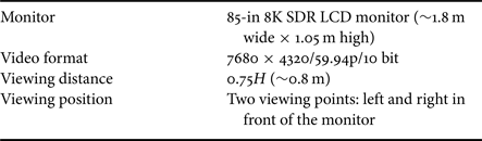
Ten 8K 60-Hz video sequences were used for the experiment, and the spatial and temporal perceptual information (SI and TI) of each sequence based on Rec. ITU-T P.910 [9] is shown in Fig. 1. The information is calculated based on the maximum standard deviation (SD) of the spatial or temporal difference in the luma component computed for each frame. In the graph, a high value indicates that the spatial or temporal complexity is high.
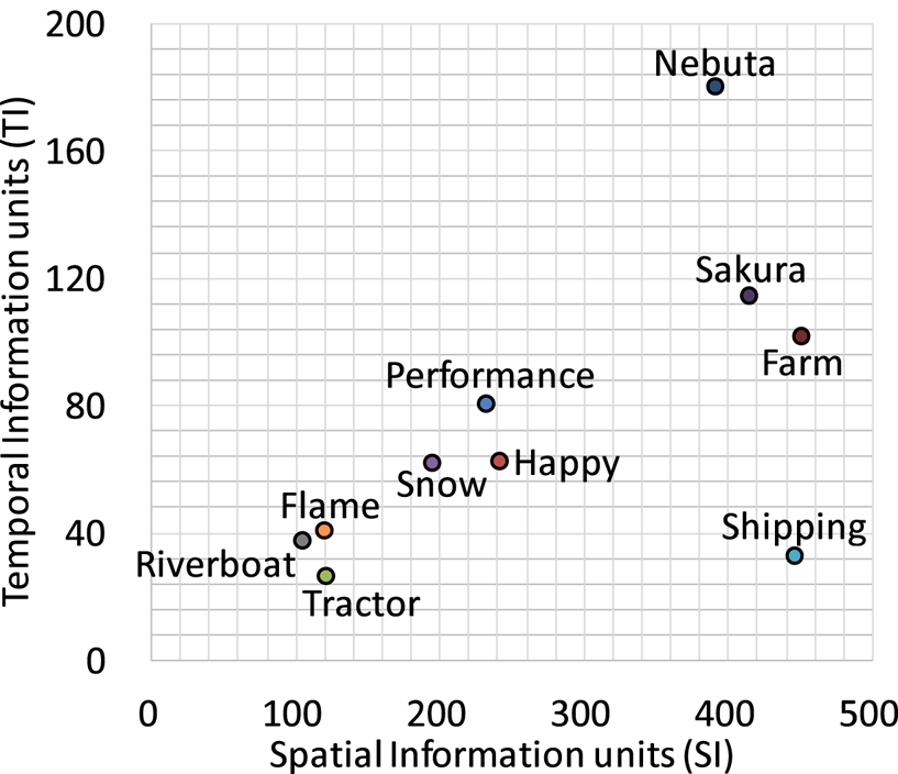
Fig. 1. Spatial and temporal perceptual information of ten 8K 60-Hz sequences.
A subjective evaluation method based on the double stimulus impairment scale (DSIS) method, Variant I described in Rec. ITU-R BT.500 [10] was used, and the presentation method is shown in Fig. 2. Twelve video coding experts participated in the evaluation. After an original (uncompressed) and encoded (compressed) videos were displayed once, each subject rated the deterioration of the encoded video relative to the original video using a five-grade scale:
1 imperceptible
2 perceptible, but not annoying
3 slightly annoying
4 annoying
5 very annoying.
Fig. 2. Presentation of videos in our experiment.
The videos were displayed on an 85-in 8K standard dynamic range (SDR) liquid crystal display (LCD) monitor. The viewing distance was set to 0.75 times the picture height (H) in consideration of the design of 8K video parameters [Reference Yamashita, Masaoka, Ohmura, Emoto, Nishida and Sugawara11] as well as an optimal viewing distance for 8K subjective assessment described in Rec. ITU-R BT.2022 [12]. To observe as many areas of the screen as possible, we considered that at least two viewing points might be required. As a result, two points were prepared to make the matter simpler (see the top view shown in Fig. 3): in total, six subjects were positioned to the left of the monitor, and six were positioned to the right.
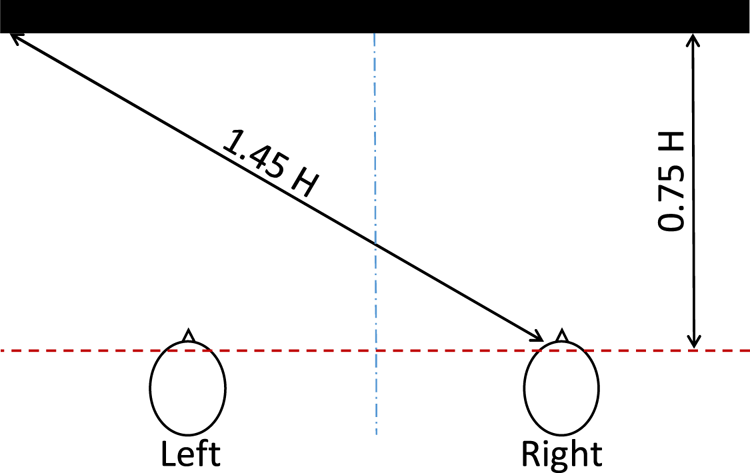
Fig. 3. 85-in 8K monitor and two viewing points at 0.75H (top view).
B) Experimental results
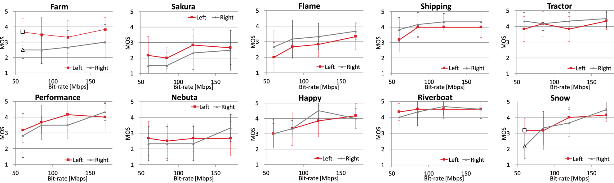
A screening method of subjects based on BT.500 [10] was conducted, and it was confirmed that there is no outlier. Figure 4 shows the experimental results for each sequence. The graphs illustrate the relationship between the bit-rate and the mean opinion score (MOS) for subjects sitting to the left (red line) and right (gray line) of the monitor. In this and the following graphs, the error bars correspond to a 95% confidence interval (CI) using the Student's t-distribution, which takes into account sample size, i.e. CI is longer at fewer sample size. Note that the MOS for each condition is commonly calculated as the combined average score of both the left and right and the corresponding CIs become shorter owing to a twice larger number of the subjects.

Fig. 4. Results of subjective evaluation experiment for 10 sequences.
As shown in the graphs, the MOS values generally differed depending on the viewing position. For five sequences (top row) out of all 10 sequences, the MOS value of one position, i.e. the left or right of the monitor, is higher than or equal to that of another position for all four bit-rates. In those five sequences, lower MOS values are assigned to parts where degradation can easily be seen.
We confirmed whether there is a statistical difference between the MOS values of the left and right (${MOS_L}$ and ${MOS_R}$
 ) using Welch's two-sided t-test. Since the test must be applied to data which follows a normal distribution, we checked that the distributions of both the left and right scores are Gaussian, after making the quantile–quantile (Q–Q) plots (we show an example of the Q–Q plot later). Here, we tested the null hypothesis:

against the alternative hypothesis
at a 5% significance level (${\alpha } = 0.05$ ) for 40 conditions (10 sequences ${\times }$
 4 bit-rates). In the lowest bit-rate of the Farm and Snow sequences, marked by a pair of white large square and triangle in each graph, ${H_0}$
 was rejected and ${H_1}$
 was adopted. In such cases, the probability values (p-values), a smaller p-value shows a lower possibility of extremer events under ${H_0}$
 , were ${p = 0.018}$
 and ${0.044}$
 , and the effect sizes (ES) ${d}$
 were 1.678 and 1.328, respectively. Since the ES values ${d}$
 were greater than 0.8, which is the criterion of large ES [Reference Cohen13], it is safe to say that the difference between ${MOS_L}$
 and ${MOS_R}$
 is sufficiently large at such two conditions.
Regarding the Snow sequence, ${MOS_L}$ and ${MOS_R}$
 fluctuate with changes in the bit-rate. Since high complexity objects exist everywhere in this sequence, e.g. snow, fountain, texture on the tiled floor, and a woman with a fine patterned umbrella, deterioration caused by compression can be seen the whole screen; however, degradation owing to the fountain on the right side might be dominant at the lowest bit-rate condition.
In addition to ranking the deterioration, the subjects were interviewed about how they observed 8K videos during the evaluation, and all of them indicated that they saw a part immediately in front of them. The subjects followed a moving object by moving their eyes and head; however, they said that it was impossible to see deterioration in another side or the entire display.
C) Considerations from results
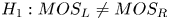
Considering the human visual system, such results, the differences of the MOS values depending on the viewing position and the answers of the interview, were reasonable. Figure 5 represents an 8K monitor and the corresponding visual field for a subject seated to the right of the monitor at a viewing distance of 0.75H. Note that Figs 5 and 6 were depicted to apply for an 8K monitor by reference to [Reference McCarthy14]. If a subject is seated directly in front of the screen, a viewing distance of 0.75H with an aspect ratio of 16:9 is equal to a 100-degree of field of view (FOV). In Fig. 5, the white circle indicates the central visual field and its diameter corresponds to an FOV of ~20$^{\circ }$ (~1500 pixels). The central high-acuity area (yellow circle) perceived by the fovea is very limited, i.e. an FOV of 6$^{\circ }$
 (~500 pixels). The spatial resolution capacity of this area is 25 or greater cycles per degree. Blind spots exist at each side of the fovea, ~15-degree of FOV from the central. Since the areas corresponding to the blind spots (blue circles) are situated within the screen, head motion, as well as eye rotation, is required to view the entire screen. Moreover, the distance to the far-left side of the monitor can be approximately twice as far as that to the right side (see Fig. 3), and this may prevent subjects from observing deterioration on the left side.
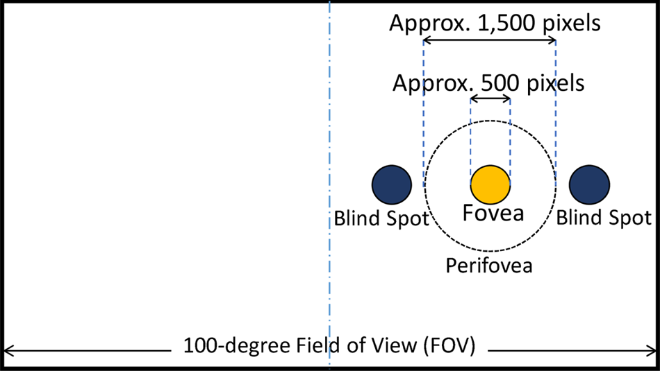
Fig. 5. 8K monitor and corresponding visual field at 0.75H.
Fig. 6. 8K monitor and corresponding visual field at 1.5H.
The viewing distance for the 8K videos (0.75H) was designed to achieve a sense of being there and to ensure that the pixel structure was not visible [Reference Yamashita, Masaoka, Ohmura, Emoto, Nishida and Sugawara11]. Whereas the selected viewing distance provides an immersive experience, it was found that subjects were forced to have a narrow view. A similar problem might be raised at an assessment of other immersive videos such as a virtual reality system, a 360-degree video, and a free-viewpoint television.
D) General subjective evaluation method for 8K encoded videos
Based on the previously described considerations, we generally conduct 8K subjective evaluation experiments for 8K encoded videos with conditions given in Table 3.
Table 3. Experimental conditions for general 8K subjective evaluations
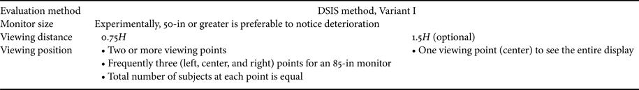
Here, we remark conditions different from the previously mentioned experiment. Regarding an 8K monitor size, experimentally, 50-in or greater is preferable. If not, deterioration of encoded videos is hardly detectable. This may be caused by a pixel density of a monitor: 104 and 176 pixel per inch for 85- and 50-in 8K monitors, respectively. Since the viewing field at 0.75H is relatively small, we frequently prepare three viewing points for an 85-in 8K monitor. Figure 7 shows the top view in such a case. In total, the same number of subjects should be assigned at each position in view of calculating the MOS values. For a subject to observe the entire display, a viewing distance of 1.5H, which is equivalent to an optimal viewing distance of 4 K videos [12], may be optionally used. An 8K monitor and the corresponding visual field of a subject at the central viewing position at a distance of 1.5H is shown in Fig. 6. In this case, a viewing distance of 1.5H with an aspect ratio of 16:9 is equal to a 60-degree of FOV, and the diameter of the central visual field corresponds to one-third of the screen width.
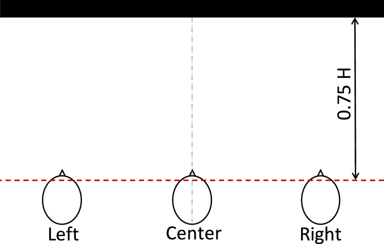
Fig. 7. 85-in 8K monitor and three viewing points at 0.75H (top view).
III. 8K 120-Hz VIDEO ENCODER FEATURES
In this section, we describe the features of our 8K 120-Hz HEVC real-time video encoder [Reference Sugito, Iwasaki, Chida, Iguchi, Kanda, Lei, Miyoshi and Uehara2]. As mentioned previously, we used video coding software that emulates this encoder for our experiments.
A) Compliance
The encoder complies with the 8K broadcasting standard (ARIB STD-B32) [1]. The standard is based on HEVC Main 10 Profile, which supports 4:2:0 10 bit encoding, and employs temporal scalable coding for 120-Hz videos that considers compatibility with 60-Hz videos.
Figure 8 shows a structure of pictures (SOP) diagram comprising 16 pictures (frame numbers 1–16) for 120-Hz videos described in the standard and a timing chart to decode and display 120- and 60-Hz videos. We used this SOP for the experiments. In Fig. 8, the numbers in rectangles are the frame numbers, the numbers above or below the rectangles indicate the encoding and decoding order, and the arrows between the rectangles indicate reference frames. Frame number 16 can be any one of intra coded picture (I picture), predictive coded picture (P picture), and bidirectionally predictive coded picture (B picture). The first frame, frame number 0, must be I picture and frame numbers 1–15 are B pictures. In this SOP, both the 120- and 60-Hz videos are decodable since only the even frames in gray or black can partially decode from the compressed 120-Hz video streams, and the 120- and 60-Hz videos can be played synchronously, as shown in the timing chart.
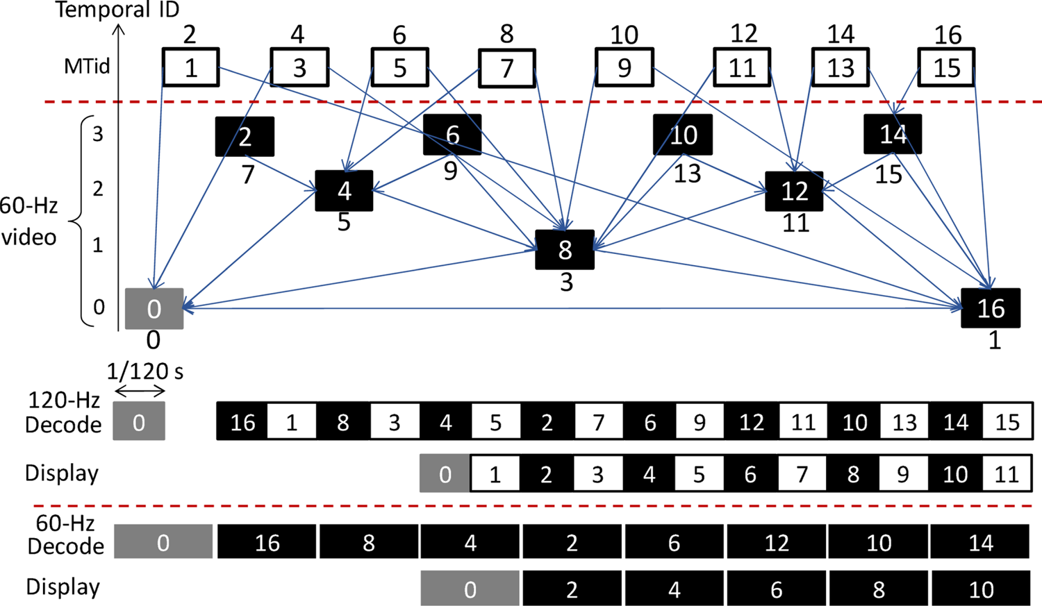
Fig. 8. SOP for 120-Hz videos and timing chart.
In addition, the standard mandates the use of a spatial division by four slices for 8K videos. The details are explained in the following sections.
B) 4 K encoder parallel processing
The 8K 120-Hz encoding process is illustrated in Fig. 9. The pre-processor divides 8K 120-Hz videos into four and three partitions in the spatial and temporal directions, respectively. The video encoding processor comprises 12 4 K 60-Hz HEVC encoders (FUJITSU IP-HE950E [15]), and each encoder processes a single spatio-temporal partition (slice).

Fig. 9. Diagram of 8K 120-Hz video encoder.
The encoding processor comprises three temporal processing groups. Each group processes at 60 Hz and encodes an SOP and the reference pictures required to encode the SOP in parallel. These reference pictures are encoded with the same parameter in each group to maintain consistency. For example, to encode the SOP shown in Fig. 8, frame number 0 is required. Then, the frame numbers 0–16 will be input frames for Group 1. To encode the next SOP with frame numbers 17–32, frame number 16 should be the reference frame, and frame number 0 is also required to encode frame number 16. Therefore, frame number 0 and frame numbers 16–32 will be input frames for Group 2. Similarly, the next SOP with frame numbers 33–48 and its reference frames, frame numbers 0, 16, and 32, will be input frames for Group 3. Although the 120-Hz frame-rate is twice that of the 60-Hz frame-rate, as the reference pictures will be encoded in their respective groups, 120-Hz real-time encoding is achieved by three 60-Hz real-time temporal encoding groups.
As shown in Fig. 9, each temporal processing group has four 4 K 60-Hz encoders. The 8K pictures are spatially divided into four slices as mandated by the 8K broadcasting standard, and each 4 K encoder processes each slice. In total, 12 encoded video streams are output from the encoding processor, and the transport stream (TS) reconstructor multiplexes the streams as an 8K 120-Hz video stream.
C) Image quality control with down-converted video
Since the 8K pictures are encoded using four slices, the differences in image quality between slices, especially on the borders of the slices, could easily be perceived as deterioration. To prevent this, the 8K broadcasting standard allows to apply a smoothing filter on such boundaries and to refer pixels on adjacent slices at inter prediction [1].
However, our encoder does not employ such technologies: 12 4 K encoders in the video encoding processor independently process each slice and do not exchange information on such borders due to the limitation of the bandwidth. To resolve this problem, the video rate controller, shown in Fig. 9, adjusts the bit allocation while analyzing the down-converted 4 K 60-Hz input video: in fact, the controller consists of a 4 K 60-Hz encoder, which is equal to the 12 4 K encoders, and the down-converted video is encoded prior to the 8K 120-Hz video. Figure 10 shows the relationship between the down-converted 4 K 60-Hz and 8K 120-Hz pictures. When encoding, the down-converted 4 K 60-Hz video is divided into four slices in the same manner as 8K videos, but each slice is able to refer to pixels on adjacent slices in inter prediction.
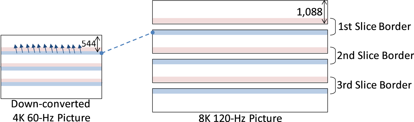
Fig. 10. Down-converted 4 K 60-Hz and 8K 120-Hz pictures.
The adjustment of the bit allocation is conducted in two steps. First, the controller estimates the complexity of each picture and slice for the 8K 120-Hz video using the encoding results of the 4 K 60-Hz video and decides the target bit amount of each slice, taking into account the actual bit amount sent from the encoding processor. Second, the controller increases the bit amount of a border area of a slice, one or more coding tree unit (CTU) lines, depending on the motion vectors of the 4 K video in the corresponding part, while maintaining the bit amount of the slice decided in the first step. For example, in Fig. 10, the motion vectors in the upper CTU line(s) of the second slice refer to the above slice, and this may cause image deterioration on the corresponding CTU line(s) in the 8K picture. This is because, in the 8K encoding process, such efficient encoding mode, which refers to the adjacent slice in inter prediction is unselectable, and selecting another inefficient way is to be forced. In that case, the controller increases the bit amount of the CTU line(s) by decreasing quantize parameter (QP) values; meanwhile, to keep the target bit-rate decided in the first step, the controller reduces the bit amount of the remaining area of the second slice by increasing QP values.
IV. EXPERIMENT 1: REQUIRED BIT-RATE FOR 8K 120-Hz VIDEOS
The purpose of Experiment 1 is to verify the required bit-rate for 8K 120-Hz videos. In this experiment, we evaluated distortions in compressed videos for four bit-rates compared to the original uncompressed videos using the general 8K evaluation method. As previously explained in Section 3.1, our 8K 120-Hz encoded streams can be viewed as both 8K 120- and 60-Hz videos. Thus, we conducted an assessment for videos with both frame-rates.
A) Test sequences
As shown in Fig. 11, we used six 8K 120-Hz test sequences for the experiments. The color space complies with Rec. ITU-R BT.2020 [16], and the image format is YC$_{{\rm B}}$ C$_{{\rm R}}$
 4:2:0 10 bit. Originally, the sequences were 15 s (1800 frames), and we encoded all the frames. However, we evaluated the middle 10 s (1200 frames) considering that the image quality at the beginning and the end of the encoded videos fluctuated due to bit-rate control. In the following description, the analysis results and the bit-rate of the sequences are described for each of the 10 s.
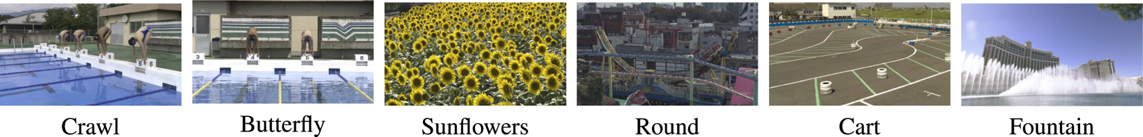
Fig. 11. Thumbnails of 8K 120-Hz test sequences.
The SI and TI of each sequence based on P.910 [9] is shown in Fig. 12. The characteristics of the six sequences spread in both spatial and temporal directions. Comparing with those of the 8K 60-Hz sequences shown in Fig. 1, the SI and TI values of 8K 120 Hz are relatively small and quite similar, respectively. Since the time interval of 120-Hz video frames is twice shorter than that of 60 Hz, the similar TI values mean that considerably rapid motion is included in the 8K 120-Hz sequences. Overall, it is found that the test sequences place emphasis on rapid motion rather than on spatial complexity.
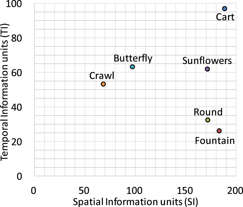
Fig. 12. Spatial and temporal perceptual information of six sequences.
B) Experimental setup
We used video coding software that emulated our 8K 120-Hz encoder and set the video coding parameters to comply with the 8K broadcasting standard [1]: HEVC Main 10 Profile, the SOP shown in Fig. 8 (I pictures were inserted every 64 frames, approximately every 0.5 s), and 8K picture partitioning with four slices (Fig. 9). Using four bit-rates (60, 85, 110, and 135 Mbps), the six 8K 120-Hz sequences were encoded. In experimental broadcasting satellite transmissions, 85 Mbps is the same bit-rate as 8K 60-Hz video [Reference Sugito, Iguchi, Ichigaya, Chida, Sakaida, Sakate, Matsuda, Kawahata and Motoyama17]. As defined by the ARIB TR-B39 ver. 1.3 8K broadcasting guideline, 110 Mbps is the maximum bit-rate for 8K 60-Hz videos. Two other bit-rates were selected such that there were equal differences.
In this experiment, the bit-rates for 8K 60-Hz videos were controlled automatically by the software. Figure 13 shows the bit allocation for 8K 120- and 60-Hz videos. In the graph, the gray parts correspond to the bit amount for the difference between 8K 120- and 60-Hz videos, and the parts in other colors are that for 8K 60-Hz videos. In each bit-rate setting, the six sequences are aligned in the descending order of the bit amount for the difference between 8K 120- and 60-Hz videos (gray parts). The differences account for from 1.2% (the Fountain sequence at 60 Mbps) to 20.4% (the Butterfly sequence at 135 Mbps) of the total bit amount. Overall, there is a tendency that the greater the total bit amount, the greater the percentage of the difference.
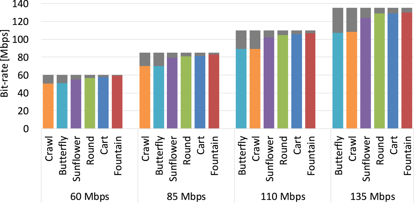
Fig. 13. Bit allocation for 8K 120- and 60-Hz videos in Experiment 1.
An 8K monitor, an 8K 120-Hz uncompressed recorder, and a 120 to 60 Hz frame-rate converter was used in this experiment, as shown in Fig. 14. The frame-rate converter which extracts the even frames shown in Fig. 8 from a recorded 8K 120-Hz video in real-time was applied for evaluations of 8K 60-Hz videos. Tables 4 and 5 show the specifications of the 8K monitor that supports a 120-Hz frame-rate and the viewing conditions, respectively.
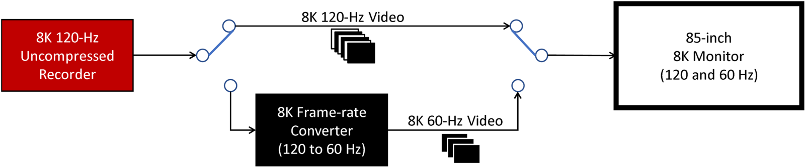
Fig. 14. Equipment for Experiment 1.
Table 4. 8K monitor specifications

Table 5. Viewing conditions of Experiment 1
In accordance with the general subjective evaluation method for 8K encoded videos discussed in Section 2.4, the evaluation method was based on DSIS Variant I described in BT.500 [10]. Figure 15 shows the presentation method during the evaluations, and the five-grade scale described in Section 2.1 was used. Twelve and 9 video coding experts participated in the 8K 120- and 60-Hz video evaluations, respectively. Note that the experimental sessions for 8K 120- and 60-Hz videos were conducted separately.

Fig. 15. Presentation method of Experiment 1.
C) Experimental results
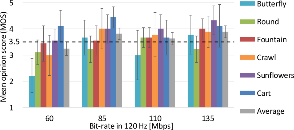
A screening method of subjects described in BT.500 [10] was conducted, and it was confirmed that there is no outlier. Figures 16 and 17 show evaluation results for the 8K 120- and 60-Hz videos, respectively. In these graphs, the vertical axis shows the MOS, and the horizontal axis is the bit-rate settings. In Fig. 17, the actual bit-rates for 60-Hz videos are less than the settings for 120-Hz videos written in the horizontal axis and are varied by sequences as shown in Fig. 13. The results demonstrate that the average of the six sequences began to exceed a MOS of 3.5, which is referred to as the acceptable threshold of distortions, at 85 Mbps for the both 8K 120- and 60-Hz videos.
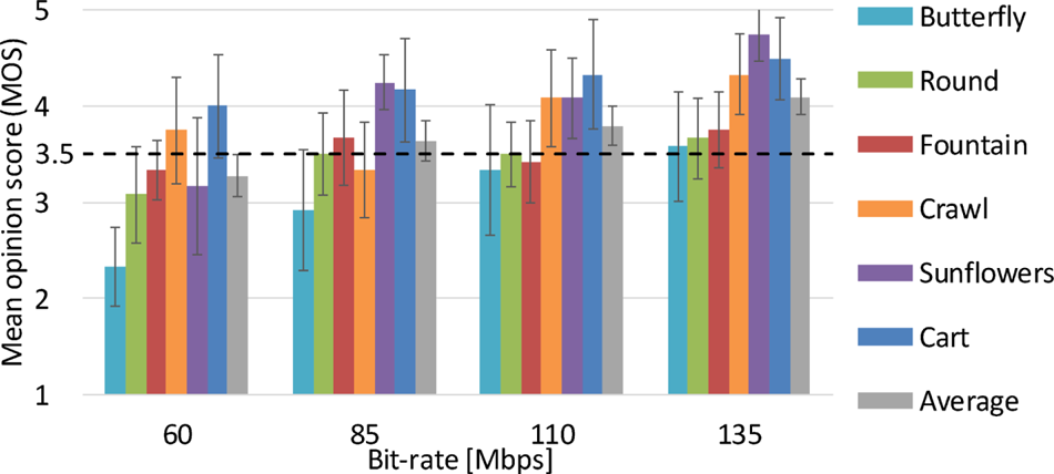
Fig. 16. Results of Experiment 1 (120 Hz).

Fig. 17. Results of Experiment 1 (60 Hz).
We also confirmed whether there is a statistical difference between the MOS values of the left, center, and right (${MOS_L}$ , ${MOS_C}$
 , and ${MOS_R}$
 ) using the one-way analysis of variance (ANOVA). Here, we tested the null hypothesis

against the alternative hypothesis

for some ${X \neq Y}$ and ${X, Y = L, C, R}$
 at a 5% significance level (${\alpha } = 0.05$
 ) for 48 conditions (6 sequences ${\times }$
 4 bit-rates ${\times }$
 2 frame-rates). Then, a multiple comparison using Tukey's test was conducted if ${H_0}$
 was rejected, i.e. ${p < 0.05}$
 . This additional test provides the minimum distance between MOS values required to be a significant difference. The results show that the two out of the 48 conditions, the Sunflowers sequence of 120 Hz at 85 Mbps (${p = 0.007}$
 ) and the Fountain sequence of 60 Hz at 85 Mbps (${p = 0.031}$
 ), were in the rejection region, and the ES values ${f}$
 were 1.225 and 1.202, respectively, which were greater than the criterion of large ES, ${f=0.40}$
 [Reference Cohen13]. Also, Tukey's test indicated the same significant differences in the viewing positions for the two conditions: ${MOS_R > MOS_C, MOS_L}$
 .
.
V. EXPERIMENT 2: APPROPRIATE BIT-RATE ALLOCATION FOR 8K 60-Hz TEMPORAL SCALABLE VIDEOS
Experiment 2 was conducted to verify appropriate bit-rate allocation for 8K 60-Hz video within the 8K 120-Hz video bit-rate. Here, “the appropriate bit-rate allocation” should maximize the image quality for both 8K 120- and 60-Hz videos. We evaluated the difference between videos compressed by three types of allocation techniques using a new subjective evaluation method.
A) Subjective evaluation method
Prior to conducting the experiment, we considered a subjective evaluation method suitable to distinguish slightly different 8K videos. In the DSIS method, the original and compressed videos are compared; however, different compressed videos are not compared. Thus, this method is not suitable for our experimental purposes.
The subjective assessment method for video quality evaluation (SAMVIQ) described in Rec. ITU-R BT.1788 [18] is a detailed approach that can be used to detect small differences between videos. In SAMVIQ, subjects can freely play and stop the reference video or the evaluation videos corresponding to the reference video until the videos under evaluation have been scored. Therefore, an integrated system with a user interface, video recorder, and monitor is required for this method; however, systems that support 8K 120- and 60-Hz videos are not available.
Another detailed subjective evaluation method is the pair comparison (PC) method described in P.910 [9]. Note that an equivalent method is described in BT.500 [10]. For PC, each pair of videos is typically presented only once or twice, and the subjects compare the videos by grading them with a relative score. Thus, a simple system with a recorder and monitor is sufficient for the PC method.
To create an evaluation method that is more detailed than normal PC and one that requires simple equipment for 8K 120- and 60-Hz videos, we tested a PC method that has desired repetitions like SAMVIQ. We refer to this as the repeatable PC (RPC) method.
We also considered how to display 8K videos in the RPC method. To compare a pair of videos, two monitors can be used to present each video; however, we found this approach is not suitable for 8K encoded video evaluations. Due to the 8K viewing distance, subjects can only see a part immediately in front of them; thus, they must switch from monitor to monitor to compare the same part of each video. Here, the moving distance is approximately the width of the monitor, e.g. at least 1.1 m given that a 50-in or greater monitor size is required, as shown in Table 3. Thus, we used a single 8K monitor for the evaluations by displaying a pair of videos in sequence.
B) Video coding conditions
Although the RPC method enables us to conduct detailed evaluations, one defect of the method is that it may take a long time to finish the assessment. Therefore, we decided to select four 8K 120-Hz sequences, the Butterfly, Cart, Round, and Sunflowers sequences, out of the six sequences in Experiment 1 in consideration of their characteristics. The Butterfly and Crawl sequences are swimming videos with camera motion, and they have similar SI and TI values (Fig. 12). So, we chose the Butterfly sequence which has a higher encoding complexity than the Crawl sequence as shown in Figs 16 and 17. The Round and Fountain sequences were shot by a fixed camera, and their SI and TI values are quite similar. Thus, the Round sequence was selected in the same manner as the previous case.
In consideration of the results obtained in Experiment 1, we encoded the four 8K 120-Hz sequences at 85 Mbps under the three conditions given in Table 6. We configured the bit-rate for the maximum Temporal ID (MTid) shown in Fig. 8, which corresponds to the difference between 8K 120- and 60-Hz videos, and the 8K 120-Hz video bit-rate. The other video coding parameters were the same as in Experiment 1.
Table 6. Video coding conditions for Experiment 2
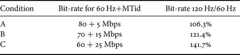
Figure 18 shows the peak signal-to-noise ratio (PSNR) and bit-rate of the three conditions and 85 Mbps setting for Experiment 1, where the vertical axis shows the average PSNR for the luma component Y over the frames. For each sequence, one of the three conditions is close to the settings of Experiment 1 (purple markers).
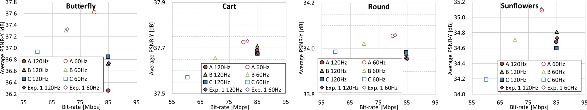
Fig. 18. PSNR and bit-rate of experimental conditions.
C) Experimental setup
Experiment 2 used the same equipment used in Experiment 1 (Fig. 14). The viewing conditions are given in Table 7. Note that each evaluation was with a single subject.
Table 7. Viewing conditions of Experiment 2
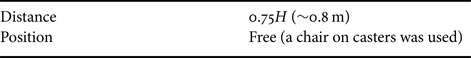
Figure 19 shows the evaluation presentation method based on P.910 [9]. As can be seen, Videos A and B are two of the three conditions, and the order effect was considered, i.e. comparisons of both Conditions B after A (A–B) and B–A were assessed. Videos A and B after the gray titles A and B shown in the figure were repeated until each subject finished grading the score. If a session continued for more than 30 min, each subject took at least a 30-min break prior to resuming evaluations.
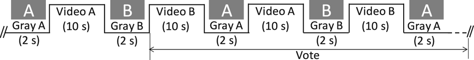
Fig. 19. Presentation method of Experiment 2.
In Experiment 2, Video B relative to Video A was evaluated using the seven-grade scale defined in BT.500 [10]. Figure 20 shows the scale on the evaluation sheet (top) and the corresponding seven-grade scores (bottom).
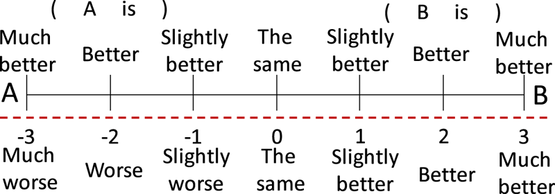
Fig. 20. Scale used for Experiment 2 and corresponding scores.
Here, nine video coding experts participated in the 8K 120- and 60-Hz video evaluations, and these experts evaluated all 24 items (${_3P_2}$ pairs ${\times }$
 4 sequences) for the two frame-rates.
D) Experimental results
We calculated MOS values and analyzed statistical differences of these values for Conditions A, B, and C using Scheffé's method modified by Ura. The method, which is ANOVA with repeated measurements, was modified to consider the order effect and to evaluate all conditions by all observers. For example, the MOS of Condition A in a sequence of a frame-rate is calculated by equation (5), where ${S_{iXA}}$ and ${S_{iAX}}$
 are the scores for X–A and A–X given by subject $i =$
 1–9, respectively, X is A, B, or C, and ${S_{iXX}}$
 is assumed to be 0.

Here, we tested the null hypothesis of the main effect

against the alternative hypothesis

for some ${X \neq Y}$ and ${X, Y = A, B, C}$
 at a 5% significance level (${\alpha } = 0.05$
 ) for 10 items (four sequences and their average for two frame-rates). To find specific conditions that have a significant difference, we further conducted multiple comparisons using Tukey's test if ${H_0}$
 was rejected, i.e. when a p-value was smaller than 0.05.
Figures 21 and 22 show the Experiment 2 analysis results for the 120- and 60-Hz videos, respectively. In these graphs, each marker shows the MOS (the theoretical range is $\pm 2$ ), and the p-value of the main effect is described under each title. The arrow above a scale represents the minimum width of a statistically significant difference, which is the result of the multiple comparison. The significant differences are indicated under the titles by the > symbol, which means that a difference between the MOS values is larger than the corresponding scale. In terms of the Butterfly sequence for 120 Hz, though the p-value was smaller than 0.05, the difference between ${MOS_A}$
 and ${MOS_C}$
 was slightly smaller than the corresponding scale.
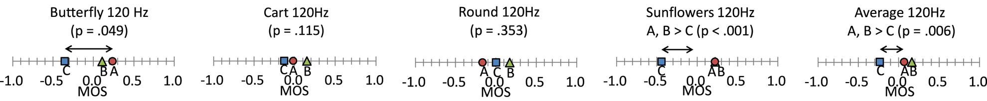
Fig. 21. Results of analysis for Experiment 2 (120 Hz).
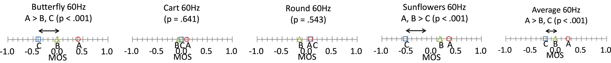
Fig. 22. Results of analysis for Experiment 2 (60 Hz).
For the 120-Hz videos, the Sunflowers sequence and the average of the four sequences demonstrate a significant difference, i.e. Conditions A and B are better than Condition C. The ES values ${f}$ are 0.658 and 0.493, respectively. With the 60-Hz videos, the Sunflowers sequence demonstrates a significant difference in the same manner as that of the 120-Hz videos, and the Butterfly sequence and the average demonstrate another significant difference, i.e. Condition A is better than Conditions B and C. The ES values f were 0.700, 0.544, and 0.656, respectively. Since the ES values f were greater than 0.4, which is the criterion of large ES [Reference Cohen13], it can be said that the differences between the MOS values are sufficiently large.
VI. CONSIDERATIONS
A) Required bit-rate for 8K 120-Hz HEVC temporal scalable coding
Here, we discuss the required bit-rate in consideration of the results obtained in Experiments 1 and 2.
1) Required bit-rate for 8K 120-Hz videos
Ichigaya and Nishida [Reference Ichigaya and Nishida4] mention criteria to achieve broadcast quality at a subjective evaluation experiment assessed by experts: (a) most of the sequences should satisfy at least a MOS of 3.5, which is referred to as “the acceptable threshold,” and at the same time, (b) no sequence should be less than a MOS of 3.0, which is referred to as the “annoying level.”
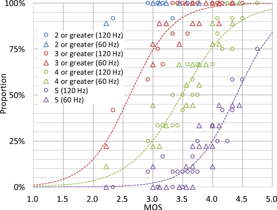
First of all, we look at what the MOS values used for the criteria statistically mean. Figure 23 illustrates the relationship between a MOS value (horizontal axis) and the proportions of scores (vertical axis) for four different ranges in Experiment 1. Each marker indicates an experimental result of a condition (e.g. the four plots at the minimum MOS value correspond to the Butterfly sequence for 60 Hz at 60 Mbps as can be seen in Figs 16 and 17). The colors of the markers correspond to the ranges of scores, namely, 2 or greater (2–5, blue), 3 or greater (3–5, red), 4 or greater (4–5, green), and 5 (purple). The shapes of the markers correspond to the frame-rates, namely, 120 Hz (circle), and 60 Hz (triangle). The dashed lines are the results of the curve fitting using the least square method. The logistic function ${\hat {y}}$ shown in equation (8) was applied, and the colors of the lines are equivalent to the ranges of scores:

where ${x}$ and ${\hat {y}}$
 are a MOS value and a predicted proportion, respectively. The true proportion ${y}$
 corresponding to ${x}$
 exists as shown in the circle or triangle markers in the graph. The variables ${a}$
 and ${b}$
 were selected to minimize ${\sum _{all \, conditions \, i} (y_i-\hat {y}_i )^2}$
 . There are 48 conditions (6 sequences ${\times }$
 4 bit-rates ${\times }$
 2 frame-rates) for each line. Note that a curve for the range of scores 2–5 was not derived due to the lack of MOS values smaller than 2.

Fig. 23. Relationship between score distribution and MOS in Experiment 1.
In general, video coding experts are sensitive to deterioration caused by compression, i.e. experts tend to grade lower scores than non-experts for low-quality images. Figure 23 shows that in MOS=3.0, almost 100% of such stern subjects rank 2 or higher scores. In other words, if a MOS is less than 3.0, there is a possibility to exist a score of 1, which means “very annoying.” Thus, this can be said that a MOS of 3.0 is a minimum level to avoid a very low quality. Also, the figure shows that in MOS=3.5, more than 90% and ~50% of subjects grade scores 3–5 and 4–5, respectively. This means that if a MOS of a condition is 3.5 or higher, more than half of subjects don't consider it as an annoying level, and almost all of the rest of the subjects perceive it as a barely annoying level.
Getting back to the criteria of (a), the results of Experiment 1 for both the 120- and 60-Hz videos demonstrate that the average of the six sequences and at least four out of the six sequences exceed the acceptable threshold of distortions, MOS=3.5, under the 85 Mbps or greater bit-rate settings. Regarding the criteria of (b), the Butterfly sequence has a MOS of less than 3.0 for 120 Hz at 85 Mbps, and all sequences for both 120 and 60 Hz exceed a MOS of 3.0 in the 110 Mbps setting. From these results, the bit-rate required for 8K 120-Hz videos with a similar difficulty relative to sequence testing is estimated as 85–110 Mbps, which means that 8K 120-Hz videos are transmittable without large distortions at a bit-rate that is equivalent to that of 8K 60-Hz videos.
2) Appropriate bit-rate allocation at 85 Mbps
The results of Experiment 2 indicate that (1) the difference between conditions is hardly detectable in the Cart and Round sequences, and the PSNR values of the two sequences exhibit small changes, as shown in Fig. 18, (2) Condition C was worse than Conditions A and B, and (3) Condition A was much better than Conditions B and C.
Thus, the bit-rate for a 60-Hz video should be the largest among the three conditions, and appropriate bit-rate allocation for a 60-Hz video in 8K 120-Hz temporal scalable video coding at 85 Mbps is assumed to be ~80 Mbps. The video bit-rate required for 8K 60-Hz broadcasting compressed with HEVC is considered to be 80–100 Mbps [Reference Ichigaya and Nishida4]. Note that the bit-rate for the 8K 60-Hz video in Condition A is 80 Mbps, and this is the same as the lower limit. In addition, the bit-rate for the 60-Hz video should not be too small, and 60 Mbps for the 60-Hz video in Condition C may cause subjective deterioration for both 120- and 60-Hz videos. As shown in Figs 13 and 18, our encoder can control bit-rate allocation automatically in the same manner as Condition A (the Fountain, Cart, Round, and Sunflowers sequences) or Condition B (the Butterfly and Crawl sequences), and the encoder does not tend to allocate small bit amount for a 60-Hz video as Condition C. Thus, we confirm that the orientation of the rate control method is appropriate, and the possibility to increase the 60-Hz Butterfly and Crawl videos should be considered.
To verify the bit-rate allocation, we calculated the Bjøntegaard delta rate (BD-rate) [Reference Bjøntegaard19], which represents the average bit-rate growth using a positive value, based on the results of previous temporal scalable video coding experiments [Reference Han20]. Table 8 shows the average, minimum, and maximum BD-rates for the case where the frame-rate was doubled.
Table 8. BD-rate on temporal scalable video coding [Reference Han20]
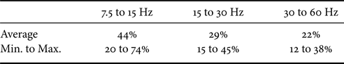
Generally, a higher frame-rate indicates higher correlation between consecutive frames and smaller bit-rate increment. As can be seen in Table 8, the average bit-rate increment from 60 to 120 Hz should be less than 20%, and it can be predicted as ~10% because the average decreases by roughly 10% in the doubled frame-rate case. Moreover, the maximum increment should be less than 40%. Considering the bit-rate increment from 60- to 120-Hz videos for each condition (third column in Table 6), the above results derived from the objective metric correspond to our subjective evaluation results.
B) Analyses on encoded videos
We analyzed encoded videos used for Experiment 1 and studied a factor to determine the subjective image quality.
1) Investigation on influence of slice borders
As previously described in Section 3.3, our encoder controls the image quality particularly on the slice borders. We hypothesized that such borders may have a large influence on the subjective image quality of the encoder.
Here, we call parts corresponding to borders of the four slices the first, second, and third slice borders as illustrated in Fig. 10. Since the 8K broadcasting standard [1] restricts referable pixels on adjacent slices to within 128 lines from the slice border, the height of each border was set to 256 lines, respective 128 lines above and below the border between the slices. As we configured the CTU size as $64\times 64$ , the 128 lines equal to 2 CTU lines. In the same manner as [Reference Sugito and Bertalmío21], we investigated the similarity between the subjective evaluation results (i.e. MOS values) in Experiment 1 and the average of the structural similarity index (SSIM) [Reference Wang, Bovik, Sheikh and Simoncelli22] for the luma component Y over the frames for each picture and slice border. As it is known that SSIM calculated after down-conversion shows better correlations with subjective evaluation results than that for images in original size [Reference Sugito and Bertalmío21,Reference Wang, Simoncelli and Bovik23], input images for SSIM were down-converted to be half size of the original images in both horizontal and vertical directions, i.e. an 8K picture was down-converted to a 4 K picture. Tables 9–11 show the Pearson linear correlation coefficient (PLCC), Spearman rank order correlation coefficient (SROCC), and root-mean-square error (RMSE) for each part of the picture, respectively. In the tables, “Picture” indicates the entire area of the 8K picture.
Table 9. PLCC for each part of picture
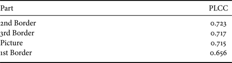
Table 10. SROCC for each part of picture
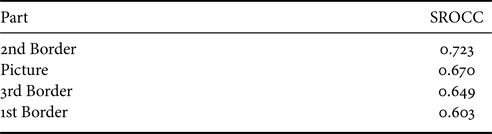
Table 11. RMSE for each part of picture
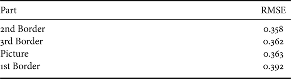
Although there is no significant difference between the four conditions, the second slice border, which is positioned in the middle of the screen height, 2049–2304th lines, showed the best results for all the three statistics. Thus, it was found that in our encoder, the image quality of the second border has larger influence than that of the entire area of the 8K picture.
2) Analysis of temporal direction
From the results of the previous section, it was confirmed that the second slice border is primarily concerned with the subjective image quality. So, it can be thought that the motion on the second border is a major cause of degradation. To verify this, we calculated the SD of frame difference for the luma component Y in the same manner as a calculation of TI [9]. Figures 24 and 25 show the SD of frame difference for the entire area of the 8K picture and on the second slice (vertical axis) calculated for each frame, respectively. Note that for each sequence, the maximum value of the SD in Fig. 24 corresponds to the TI value in Fig. 12.
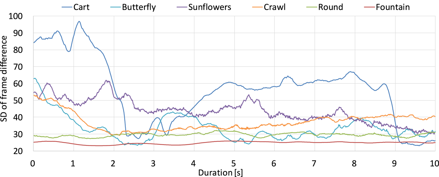
Fig. 24. SD of frame difference.
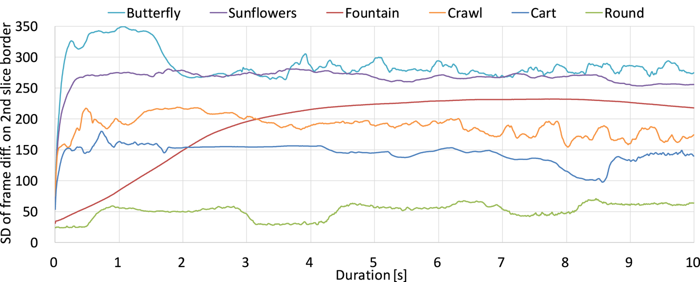
Fig. 25. SD of frame difference on 2nd slice border.
In Fig. 24, the SD values of the Butterfly, Cart, Crawl, and Sunflowers sequences fluctuate and achieve more than 50. This is because the four sequences include camera motion. In such sequences, the ranking of the temporal complexity on the second slice shown in Fig. 25 corresponds to the subjective evaluation results for 120 Hz at 60 Mbps (see Fig. 16), which should be the most notable condition of deterioration: the higher the complexity, the lower the MOS value. Notably, the Butterfly sequence showed the MOS value of less than 2.5, and the primary cause might be vertical motions crossing the slice borders caused by jumping into the pool at the beginning of the sequence. The SD values of the Butterfly sequence at the initial 2 s in Fig. 25 reflect the difficulty well. On the other hand, the SD values of the Fountain and Round sequences in the figure do not. Since the two sequences were shot by a fixed camera, the encoding complexity is relatively low in a normal situation. However, as these sequences include a random noise due to the camera characteristics, this makes the MOS values small. Also, the influence of the noise can be seen as stable low PSNRs of the Round sequence in Fig. 18. In the future, we are planning to add a noise reduction technique to our encoder as a function of the pre-processor, and the methods may improve both the coding efficiency and the image quality of those sequences.
C) Experimental conditions for 8K subjective evaluations using the DSIS method
We further analyzed the results of 8K subjective evaluation experiments using the DSIS method and considered experimental setups.
1) Number of viewing positions
In Experiment 1, we prepared three viewing points at 0.75H, and a significant difference between MOS values was statistically shown in some conditions (Section 4.3) as with the initial experiment in Section 2.2. The differences were sufficiently notable in light of their large ES values. Thus, it is reasonable to assess 8K encoded videos using two or greater viewing positions also in the future. Moreover, the number of viewing points may also be determined by the monitor size. For example, the width of a 50-in monitor is ~1.1 m, and that is not enough to align three viewing positions, i.e. three evaluators, in a straight line.
2) Number of subjects
BT.500 [10] recommends using at least 15 observers, while it also allows using those of fewer than 15 for mainly exploratory purposes. In this paper, we conducted subjective evaluation experiments using twelve or nine video coding experts, and this corresponds to the latter case.
In addition to this, the number of subjects can be determined by statistical power analysis. In this method, one of the variables, sample size (${N}$ ), significance level (${\alpha }$
 ), effect size (ES), and statistical power ($1-{\beta }$
 ), can be derived from the other three variables. We conducted power analyses using G*Power [Reference Faul, Erdfelder, Lang and Buchner24]. The statistical power ($1-{\beta }$
 ), which represents the probability of rejecting a false null hypothesis correctly, is generally set as 0.80 or more [Reference Cohen13]. Also, the variable ${\beta }$
 indicates the probability of the type II error, whereas the variable ${\alpha }$
 shows that of the type I error. These two values are in a trade-off relationship.
In general, the number of subjects ${N}$ should not be too large, considering that it takes a long time for subjective evaluations. For Experiment 1, we tested a difference between MOS values of three viewing positions at ${\alpha =0.05}$
 , and the ES values ${f}$
 were ~1.2, as shown in Section 4.3. In such cases, the minimum number of subjects to achieve ${1-\beta =0.8}$
 is 12. Therefore, the number of evaluators for 120-Hz videos in Experiment 1 was sufficient to prove the hypothesis test, and at least 15 observers will be required for future experiments so that it complies with the recommendation.
If two viewing points are used, the minimum number of subjects to study the difference between MOS values can be estimated using the ES values ${d}$ shown in Section 2.2: 20 for ${d=1.328}$
 and 14 for ${d=1.678}$
 . Thus, from 16 to 20 subjects will be required for future experiments so that it complies with the recommendation, and the number of subjects in each position is to be equal.
D) Experimental conditions for 8K subjective evaluations using the RPC method
We further analyzed the results of Experiment 2 and considered experimental settings using the RPC method.
1) Confirmation of occurrence of order effect
The order effect is caused by the presentation order of evaluation videos. In Experiment 2, all pairs of conditions were evaluated as described in P.910 [9], which considers the order effect. However, we hypothesized that the effect may become weak and negligible in the RPC method because the videos can be repeated many times.
Thus, a dependent two-sided t-test was conducted on the mean difference of each combination, i.e. the mean difference between ${S_{iXY}}$ and ${-S_{iYX}}$
 , where ${S_{iXY}}$
 is the score for X–Y given by subject $i =$
 1–9 and XY is AB, BC, or AC. Here, we tested the null hypothesis

against the alternative hypothesis

where ${\overline {S_{XY}-(-S_{YX})}}$ is the mean of ${S_{iXY}-(-S_{iYX})}$
 for 24 items (4 sequences ${\times }$
 3 combinations ${\times }$
 2 frame-rates) at a 5% significance level ($\alpha =0.05$
 ). Since the test is premised on normal distribution of data, we confirmed it previous to the test. Figures 26 and 27 show the distribution of differences of all combinations (i.e. all ${S_{iXY} + S_{iYX}}$
 ) and the Q–Q plot of the differences, respectively. The Q–Q plot roughly appears as a straight line, which confirms that the data can be assumed to have normal distribution.
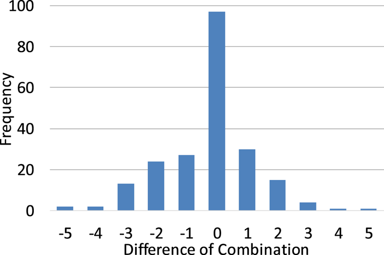
Fig. 26. Distribution of differences of all combinations.
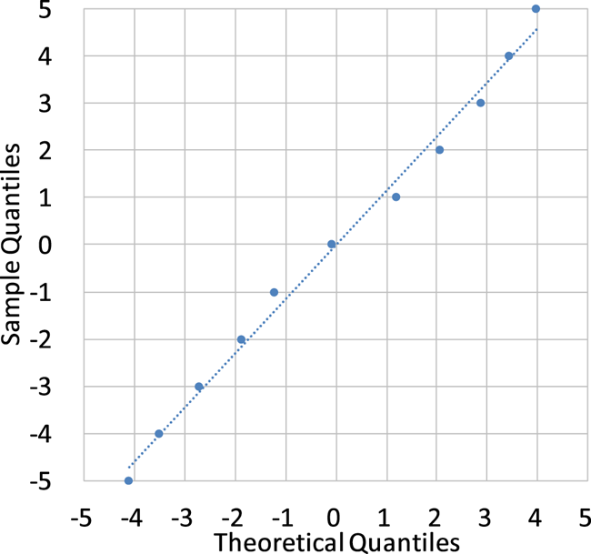
Fig. 27. Q–Q plot of differences of all combinations.
The two out of the 24 items, the combination AB of the Butterfly sequence of 120 Hz and the combination BC of the Sunflowers sequence of 60 Hz, were in the rejection region (${p = 0.038}$ and ${0.030}$
 , respectively). The ES values ${d}$
 were 0.825 and 0.875, respectively, which is greater than the criterion of large ES (${d = 0.8}$
 ) [Reference Cohen13]. Thus, it is safe to say that the mean differences are sufficiently large. The results demonstrate that the order effect is not negligible; therefore, in the RPC method, all pairs of conditions must be evaluated also in the future.
2) Number of grade scale
With the RPC method, we used the seven-grade scale written in BT.500 [10] (Fig. 20). To consider the possibility of reducing the number of a grade scale, we analyzed the results of Experiment 2 using the Bradley–Terry (BT) model [Reference Handley25, Reference Li, Barkowsky and Le Callet26].
In the BT model, $\pi _{XY}$ , i.e. the probability that Condition X is better than $Y (X \neq Y$
 and $X,Y=A, B, C)$
 , can be defined as follows:

where $\pi _X, \pi _Y > 0$ and $\sum _{X=A}^{C}\pi _X=1$
 . The BT score for Condition X $V_X$
 , which represents its merit, can be calculated as follows:

In equations (11) and (12), $\pi _{X}$ can be solved iteratively after counting the total number of comparisons preferring Condition X $a_X$
 from the results of Experiment 2. Here, we counted the variables as follows:

Note that this corresponds to a three-grade scale. We conducted a two-sided chi-square test to confirm whether there is a significant difference between the three merits. We tested the null hypothesis

against the alternative hypothesis

for some ${X \neq Y}$ and ${X, Y = A, B, C}$
 at a 5% significance level (${\alpha } = 0.05$
 ) for 10 items (4 sequences and their average for 2 frame-rates). To be more specific, ${a_{XY}}$
 (XY is AB, BC, or AC), which describes the total number of comparisons preferring Condition X over Condition Y, should be equal to $a_{YX}$
 under ${H_0}$
 . We calculated the chi-square values using such expected values and ${a'_{XY}}$
 derived from ${\pi _X}$
 and ${\pi _Y}$
 . When ${H_0}$
 was rejected, i.e. a p-value was smaller than 0.05, we further conducted multiple comparisons using the residual analysis to find a specific pair of conditions that shows a significant difference.
Figure 28 shows the analysis results for Experiment 2 obtained using the BT model. As shown in the p-values under the titles, for the 120-Hz videos, the Butterfly and Sunflowers sequences and the average of the four sequences were in the rejection region. The ES values ${w}$ were 0.869, 0.640, and 0.885, respectively, which were greater than the criterion of large ES, ${w=0.5}$
 [Reference Cohen13]. For the 60-Hz videos, the same conditions as those of 120 Hz showed the p-values smaller than 0.05, and the ES values ${w}$
 were 0.833, 0.910, and 0.888, respectively.
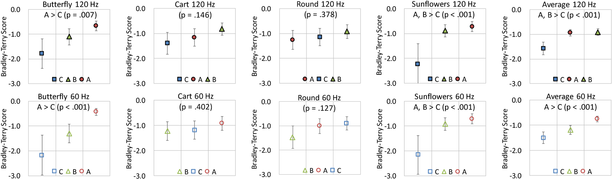
Fig. 28. Results of analysis of Experiment 2 usingthe BT model.
Comparing with the results shown in Figs 21 and 22, the Sunflowers sequence of 120 and 60 Hz and the average of 120 Hz showed the same significant differences: A, B, > C. The Butterfly sequence of 60 Hz and the average of 60 Hz do not indicate a significant difference for A>B. On the other hand, the Butterfly sequence of 120 Hz newly demonstrates a significant difference for A>C. In summary, the results using the BT model indicate that Condition A was the best and Condition C was the worst among the three conditions.
From these results, we confirm that similar significant differences are detectable if we consider the seven-grade scale of Experiment 2, i.e. $-3$ to $+3$
 , as a three-grade scale, i.e. $-1$
 , 0, and $+1$
 . This may mean that the ratio of the scores ±2 and 3 was small in the experiment (the frequency was 11%). The subjects may have been able to score ±1 for a slight difference due to extreme scores, e.g. ±3. In that case, if RPC is conducted with a three-grade scale, instructions to encourage the subjects to actively score ±1 for subtle differences would be required.
3) Number of subjects
In the same manner as Section 6.3.2, we estimated the number of subjects for future experiments using G*Power [Reference Faul, Erdfelder, Lang and Buchner24]. In Section 5.4, we tested a significant difference between conditions using ANOVA with repeated measurements, and the ES values ${f}$ were from 0.493 to 0.700. In such cases, the minimum number of subjects to achieve ${1-\beta =0.8}$
 is from 6 to 10. Thus, the number of subjects in Experiment 2, nine, was partially sufficient for the analysis. Considering the number of subjects described in BT.500 [10], 15 subjects should be prepared for future experiments with the same settings as Experiment 2.
Also, in the previous section, we confirmed a significant difference between conditions using the chi-square test. The ES values ${w}$ were from 0.640 to 0.910, and the minimum number of subjects to achieve ${1-\beta =0.8}$
 is from 10 to 20, which is larger than those in the seven-grade scale case. Thus, from 15 to 20 subjects will be required for future experiments if we use a three-grade scale.
VII. CONCLUSIONS
In this study, we encoded 8K 120-Hz sequences using software equivalent to a real-time encoder and conducted two types of informative subjective evaluation experiments to ensure the bit-rate required for 8K 120-Hz temporal scalable video coding. The experimental results confirm that the bit-rate required for 8K 120-Hz videos is 85 to 110 Mbps, which is equivalent to the practical bit-rate for 8K 60-Hz videos, and the appropriate bit-rate allocation for 8K 60-Hz videos in 8K 120-Hz temporal scalable video coding at 85 Mbps is assumed to be ~80 Mbps. The requirements are applicable to 8K 120-Hz videos which have a similar difficulty in the test sequences used for the experiments. From the analyses of the encoded videos, it was confirmed that the image quality on the slice boundary in the middle of the screen height has a large influence on the subjective evaluation results. Additionally, it was found that the encoding complexity of a sequence is related to the motions on such boundary. This may be a clue to improve the image quality of our encoder.
When conducting the experiments, we used some special settings taking into account the viewing distance of 8K videos. We analyzed the results of the experiments and considered experimental conditions for 8K subjective evaluations: preparing two or greater viewing positions is desirable also in the future. We estimated the number of subjects required for future experiments which complies with the recommendation and satisfies statistical requirements.
We also confirmed that the encoder achieved good base image quality without referring pixels on adjacent slices. In the future, we plan to evaluate the real-time encoder using other types of sequences, such as high dynamic range videos. In addition, we plan to improve the encoder's image quality reflecting those experimental results.
ACKNOWLEDGMENTS
The authors would like to thank Enago (www.enago.jp) for the English language review.
CONFLICT OF INTEREST
None.
ETHICAL STANDARD
The authors assert that all procedures contributing to this work comply with the ethical standards of the relevant national and institutional committees on human experimentation and with the Helsinki Declaration of 1975, as revised in 2008.
Yasuko Sugito is currently with NHK (Japan Broadcasting Corporation) Science and Technology Research Laboratories, Tokyo, Japan, researching video compression algorithms and image processing on 8K. Her current research interests focus on image quality assessment for high frame-rate (HFR) 8K 120-Hz videos and high dynamic range (HDR) images.
Shinya Iwasaki received a master's degree in computer science and engineering from Waseda University in 2014. Currently he works with NHK (Japan Broadcasting Corporation) Science and Technology Research Laboratories, Tokyo, Japan. His main research interests are ultrahigh definition television system and video coding.
Kazuhiro Chida received his B.S. and M.S. degrees in Information and Communication Engineering from The University of Electro-Communications, in 2007 and 2009, respectively. Currently he works with NHK (Japan Broadcasting Corporation) Science and Technology Research Laboratories, Tokyo, Japan. His main research interests are video coding and ultrahigh definition television system.
Kazuhisa Iguchi received his B.S. and M.S. degrees in electrical engineering from Tokyo Institute of Technology, in 1991 and 1993, respectively. He joined NHK (Japan Broadcasting Corporation), Tokyo, Japan in 1993, and has been working at NHK Science and Technology Research Laboratories. Heis engaged in the research of television standards conversion for HDTV, scene description, and moving picture coding.
Kikufumi Kanda received a master's degree in electrical engineering from Sophia University in 1992. Currently he works with NHK (Japan Broadcasting Corporation) Science and Technology Research Laboratories, Tokyo, Japan. His main research interests are ultrahigh definition television system and video coding.
Xuying Lei received a master's degree in Information and Communication Engineering from Kanazawa University in 2011. Currently she works with Fujitsu Laboratories Ltd. (Kanagawa, Japan). Her work focuses specifically on performance optimization during 8K Ultra-high-definition video encoding and compression.
Hidenobu Miyoshi is currently with Fujitsu Laboratories Ltd. (information and communication technology company), Kanagawa, Japan, researching data transmission and processing system. His main research interests are data management in the cloud and applications of video coding and image processing.
Kimihiko Kazui received a master's degree in electrical engineering from the Tokyo Institute of Technology in 1993. Currently he works with Fujitsu Laboratories Ltd. His research interest is video coding and he has been participatingin several standardization activities.


 Open access