


Introduction
Reflections on the limitations and shortcomings of current research practices have become common in social science research. The more general framework of the so-called metascience research is scrutinising research practices intending to improve the reliability and reproducibility of findings. Like other contingent disciplines, behavioural science has grappled with a crisis concerning the effect sizes of research findings (e.g. Maier et al., Reference Maier, Bartoš, Stanley, Shanks, Harris and Wagenmakers2022). This crisis, often known as the effect size crisis, highlights the frequent overestimation of the magnitude and significance of the effects under study. The main concern in behavioural research and experiments has been the large body of small effect sizes of treatments that need to be statistically validated. Researchers might report disproportionately significant effect sizes that are rarely replicable and often vanish or shrink significantly in subsequent, more robust studies. There is a long-standing debate about effect size in psychology that has shaped the research practices of the past years (Kelley and Preacher, Reference Kelley and Preacher2012, Westfall et al., Reference Westfall, Kenny and Judd2014, Van Bavel et al., Reference Van Bavel, Brady and Reinero2016, Schäfer and Schwarz, Reference Schäfer and Schwarz2019). In general, we can identify aspects related to the problem of making behavioural findings more robust. The first concern is the issue of treatment selections. As behavioural research is meant to be applied, selecting and testing a given treatment in a randomised controlled trial is, at best, often compared to a couple of other alternatives. Therefore, the relative effectiveness of the treatment, given the overwhelmingly small effect sizes found in behavioural studies, is difficult to assess when the efficacy of alternative treatments remains unknown. An answer to the selection problem has been the introduction of the ‘mega-studies’ (Milkman et al., Reference Milkman, Gromet, Ho, Kay, Lee, Pandiloski, Park, Rai, Bazerman, Beshears, Bonacorsi, Camerer, Chang, Chapman, Cialdini, Dai, Eskreis-Winkler, Fishbach, Gross and Duckworth2021). These are large-scale studies that simultaneously test many treatments or interventions. Mega-studies’ power lies in trying to overcome the selection bias of treatments, their increased statistical power to detect even small effect sizes and their ability to provide more accurate estimates. Furthermore, they allow researchers to assess the consistency of effects across various experimental conditions and populations. Yet, despite these advantages, mega-studies also carry challenges, such as complex data management and analysis, and they may inadvertently inflate type I errors if multiple testing corrections are not appropriately applied.
One issue often neglected in both conventional and large-scale studies is the examination of heterogeneity in treatment effects. Heterogeneity of treatment effects refers to the variability in how different subgroups within a sample respond to an intervention or treatment. For example, a certain behavioural intervention might be effective for one demographic group but not for another. By failing to analyse this heterogeneity with sophistication, researchers may miss crucial insights and patterns in the data that have practical implications (see Schimmelpfennig et al., Reference Schimmelpfennig, Vogt, Ehret and Efferson2021; Steinert et al., Reference Steinert Janina, Sternberg, Prince, Fasolo, Galizzi Matteo, Büthe and Veltri Giuseppe2022; Athey et al., Reference Athey, Keleher and Spiess2023). According to some behavioural scientists (Bryan et al., Reference Bryan, Tipton and Yeager2021; Hallsworth, Reference Hallsworth2023; Hecht et al., Reference Hecht, Dweck, Murphy, Kroeper and Yeager2023), behavioural science must address that most treatment effects are heterogeneous. It is essential to incorporate sophisticated heterogeneity treatment effects analysis in traditional and mega-studies to offer a nuanced view of the population under study, recognising individuals’ diversity and unique characteristics of the population's milieus. Doing so provides more precise estimates of effect sizes and offers insights into potential moderators and mediators of these effects. Sophisticated analysis of these effects can yield insights missed in studies only seeking to establish the average treatment effect (ATE) (Ding et al., Reference Ding, Feller and Miratrix2019). Treatment effects can differ based on various factors, including demographics, cultural background and even genetic variations, as socio-genetics studies claim. Despite the importance of this variability, it has yet to be analysed with sophistication in behavioural research. It is more analytically complex to analyse beyond comparing two or three groups defined by categorical variables. This paper will discuss analytical strategies developed in the context of computational social science that will benefit the behavioural scientist. We will discuss the methodological rationale and provide simulations to illustrate the points.
Computational social science methods for heterogeneity analysis
As mentioned in the previous section, the challenge of implementing the heterogeneity analysis approach in methodological terms is not easy. Help, however, comes from the new analysis techniques that have emerged in the computational and computer sciences and their application in social sciences. There is a larger discussion about the transformative aspect of computational social science on the modelling practices of social scientists. In summary, the predominant modelling culture in the social sciences has been defined as the data modelling culture or DMC in contrast with the emerging algorithmic modelling culture or AMC (Breiman, Reference Breiman2001; Veltri, Reference Veltri2017). The convergence process between these two modelling cultures is an object of the aforementioned discussion. First, the emphasis on ‘explainability’ using simpler statistical models with reduced predictive power is increasingly questioned (Hofman et al., Reference Hofman, Sharma and Watts2017). Hence, the hybrid approach argues that we should think about models in terms of their validation in terms of prediction, which means embedding better practices of increasing reliable, valid and replicable causal inferences in the social sciences. Future social scientists will need to be acquainted with the logic of predictive modelling developed in machine learning techniques. There is a renovated emphasis on identifying causal relationships in the social sciences. This is due to the increased use of experiments, particularly in the form of randomised controlled trials (RCT), partly due to the digital data revolution. All sorts of social scientists now run different forms of online experiments (Veltri, Reference Veltri2023). Large-scale experiments are part of the testing phase of public policy development, and, in general, the search for the identification of causal effects has become increasingly important. The traditional concerns about the external and ecological validity of experiments have been surpassed by the capacity to run experiments outside the lab and, at the same time, increase the granularity of measurements. Outside academia, digital platforms have already entered the age of big experimentation, running literally thousands of experiments, the so-called A/B testing, to continuously improve the way platforms can shape their users’ behaviour. At the same time, advancements in causal inference modelling have produced several new approaches tailored to inferring causality from observational data (Pearl, Reference Pearl2010; Imbens and Rubin, Reference Imbens and Rubin2015; Peters et al., Reference Peters, Janzing and Schölkopf2017; Hernan and Robins, Reference Hernan and Robins2024). The same effort is behind the increased sophistication in determining causal effects in experimental data that will be discussed later in this paper. One approach to how social and behavioural sciences can benefit from analytical approaches developed in the context of computational methods is the development of model-based recursive partitioning. This approach is an improvement in the use of classification and regression trees. The latter also being a method from the ‘algorithmic culture’ of modelling that has useful applications in the social sciences but is essentially data-driven (Berk, Reference Berk2006; Veltri, Reference Veltri2023). In summary, classification and regression trees are based on a purely data-driven paradigm. Without using a predefined statistical model, such algorithmic methods recursively search for groups of observations with similar values to the response variable by constructing a tree structure. They are very useful in data exploration and express their best utility in the context of very complex and large data sets. However, such techniques make no use of theory in describing a model of how the data were generated and are purely descriptive, although far superior to the ‘traditional’ descriptive statistics used in the social sciences when dealing with large datasets.
Tree-based methods
Model-based recursive partitioning (Zeileis et al., Reference Zeileis, Hothorn and Hornik2008) represents a synthesis of a theoretical approach and a set of data-driven constraints for theory validation and further development. In summary, this approach works through the following steps. Firstly, a parametric model is defined to express a set of theoretical assumptions (e.g. through a linear regression). Second, this model is evaluated according to the recursive partitioning algorithm, which checks whether other important covariates that would alter the parameters of the initial model have been omitted. The same regression or classification tree structure is produced. This time, instead of partitioning by different patterns of the response variable, it creates different versions of the parametric model in terms of β estimation, depending on the different important values of the covariates. (For the technical aspects of how this is done, see Zeileis and Hornik, Reference Zeileis and Hornik2007.) In other words, the presence of splits indicates that the parameters of the initial theory-driven definition are unstable and that the data are too heterogeneous to be explained by a single global model. The model does not describe the entire dataset.
Classification trees look for different patterns in the response variable based on the available covariates. Since the sample is divided into rectangular partitions defined by the values of the covariates and since the same covariate can be selected for several partitions, classification trees can also evaluate complex interactions and non-linear and non-monotonic patterns. The structure of the underlying data generation process is not specified in advance but is determined in an entirely data-driven manner. These are the key distinctions between classification and regression trees and classical regression models. The approaches differ, firstly, with respect to the functional form of the relationship, which is limited, for example, to the linear influence of covariates in most parametric regression models and, secondly, with respect to the pre-specification of the model equation in parametric models. Historically, the basis for classification and regression trees was first developed in the 1960s as Automatic Interaction Detection (Morgan and Sonquist Reference Morgan and Sonquist1963). Later, the most popular algorithms for classification and regression trees were developed by Quinlan (Reference Quinlan1993) and Breiman et al. (Reference Breiman, Friedman, Olshen and Stone1984). Here we focus on a more recent framework by Hothorn et al. (Reference Hothorn, Hornik and Zeileis2006), based on the conditional inference theory developed by Strasser and Weber (Reference Strasser and Weber1999). The main advantage of this approach is that it avoids two fundamental problems of previous classification and regression tree algorithms: variable selection bias and overfitting (see, e.g. Strobl et al., Reference Strobl, Wickelmaier and Zeileis2009).
Hothorn et al.'s (Reference Hothorn, Hornik and Zeileis2006) algorithm for recursive binary partitioning can be described in three steps: first, starting with the entire sample, the global null hypothesis that there is no relationship between any of the covariates and the response variable is assessed. If no violation of the null hypothesis is detected, the procedure stops. If, on the other hand, a significant association is discovered, the variable with the largest association is chosen for splitting. Secondly, the best cutpoint in this variable is determined and used to split the sample into two groups according to the values of the selected covariate. Then the algorithm recursively repeats the first two steps in the subsamples until no more violation of the null hypothesis or a minimum number of observations per node are reached. In the following, we briefly summarise which covariates can be analysed using classification and regression trees, how the variables are selected for splitting and how the cutpoint is chosen. Classification trees look for groups of similar response values with respect to a categorical dependent variable, while regression trees focus on continuous variables. Hothorn et al. (Reference Hothorn, Hornik and Zeileis2006) point out that their conditional inference framework can also be applied to ordinal and censored survival time situations and multivariate response variables. Within the resulting tree structure, all respondents with the same covariate values – represented graphically in a final node – obtain the same prediction for the response, i.e. the same class for categorical responses or the same value for continuous response variables.
The next question is how the variables for potential splits are chosen and how the relevant cutpoints can be obtained. As described above, Hothorn et al. (Reference Hothorn, Hornik and Zeileis2006) provide a statistical framework for tests applicable to various data situations. In the recursive binary partitioning algorithm, each iteration is relative to a current data set (from the entire sample), where the variable with the highest association is selected by means of permutation tests as described below. The use of permutation tests makes it possible to evaluate the global null hypothesis H0 that none of the covariates has an influence on the dependent variable. If H0 is valid (in other words, if the independence between any of the covariates Zj (j = 1, . . . , l) and the dependent variable Y cannot be rejected), the algorithm stops. Thus, the statistical test acts both for variable selection and as a stopping criterion. Otherwise, the strength of the association between the covariates and the response variable is measured in terms of p-value, which corresponds to the partial null hypothesis test that the specific covariate is not associated with the response. Thus, the variable with the smallest p-value is selected for the next split. The advantage of this approach is that the p-value criterion guarantees an unbiased selection of variables regardless of the measurement scales of the covariates (see, e.g. Hothorn et al., Reference Hothorn, Hornik and Zeileis2006; Strobl et al., Reference Strobl, Boulesteix and Augustin2007 2009). Permutation tests are constructed by evaluating the test statistic for the data given under H0. Monte Carlo or asymptotic approximations of the exact null distribution are used to calculate p-values (see Strasser and Weber, Reference Strasser and Weber1999; Hothorn et al., Reference Hothorn, Hornik and Zeileis2006, for more details). After the variable for the split has been selected, we need a cutpoint within the range of the variable to find the subgroups that show the strongest difference in the response variable. In the procedure described here, the cutpoint selection is also based on the permutation test statistic: the idea is to calculate the two-sample test statistic for all potential splits within the covariate. In the case of continuous variables, it is reasonable to limit the studied splits to a percentage of potential cutpoints; in the case of ordinal variables, the categories’ order is considered. The resulting split lies where the binary separation of two data sets leads to the highest test statistic. This reflects the largest discrepancy in the response variable concerning the two groups. In the case of missing data, the algorithm proceeds as follows: observations with missing values in the currently evaluated covariate are ignored in the split decision, while the same observations are included in all other algorithm steps. The class membership of these observations can be approximated using so-called surrogate variables (Hothorn et al., Reference Hothorn, Hornik and Zeileis2006; Hastie et al., Reference Hastie, Tibshirani and Friedman2008).
MBRP or Model-based recursive partitioning was developed as an advancement of classification and regression trees. Both methods come from machine learning, which is influenced by statistics and computer science. The algorithmic logic behind classification and regression trees is described by Berk (Reference Berk2006, p. 263) as follows: ‘With algorithmic methods, there is no statistical model in the usual sense; no effort is made to represent how the data were generated. And no excuse is offered for the absence of a model. There is a practical data analysis problem to be solved that is attacked directly with procedures designed specifically for this purpose’. In this sense, classification and regression trees are purely data-driven and exploratory – thus marking the complete opposite of the model specification theory-based approach prevalent in the empirical social sciences. However, the advanced model-based recursive partitioning method combines the advantages of both approaches: first, a parametric model is formulated to represent a theory-driven research hypothesis. Then, this parametric model is handed over to the model-based recursive partitioning algorithm that checks whether other relevant covariates have been omitted that would alter the model parameters of interest. Technically, the tree structure obtained from the classification and regression trees remains the same for model-based recursive partitioning. The model-based recursive division finds different patterns of associations between the response variable and other covariates that have been pre-specified in the parametric model. Trees, in this technique, show how the relationship between the dependent variable and two independent variables changes considerably (statistically significant, as indicated by the p-values) in the different subdivisions of the sample of respondents. For example, if the relationship between the dependent variable and each independent variable changes signs for certain partitions of the dataset represented by the subgroups, a one-size-fits-all approach is highly problematic.
Causal machine learning
The evolution of model-based recursive partitioning for causal estimation led to the so-called causal tree approach. Causal Trees are a novel concept in computational social science that aims to enhance the understanding and visualisation of causal relationships in complex data. This approach builds on the traditional decision tree methodology by focusing not only on predicting outcomes but also on identifying the causal effect of an intervention or variable of interest. The fundamental goal of Causal Trees is to understand the impact of a specific treatment or intervention on different subgroups in a population. They help identify heterogeneity in treatment effects, thus enabling decision-makers to personalise interventions based on individual or group characteristics. Essentially, these algorithms are designed to answer the question: for whom does this intervention work best? Causal Trees are an expansion of the previously discussed MBRP. However, unlike standard MBRP trees that aim to minimise prediction error, Causal Trees use a splitting criterion based on potential outcomes and treatment effects. The trees identify subgroups or ‘leaves’ with similar characteristics where the treatment effect is most significant. Therefore, instead of producing a single ATE, they provide local average treatment effects (LATE) or conditional average treatment effects (CATE), allowing a more nuanced understanding and application of the treatment.
A notable contribution to this field has been made by Athey and Imbens in their paper ‘Recursive partitioning for heterogeneous causal effects’ (Athey & Imbens, Reference Athey and Imbens2016). They proposed a new method, Causal Trees or CT and an accompanying algorithm, Causal Forests. Causal Trees are used for partitioning the data into homogenous groups with regard to the treatment effect, and Causal Forests are an extension of this, using a random forest approach to provide more reliable and precise estimates. Wager and Athey later furthered the idea in ‘Estimation and Inference of Heterogeneous Treatment Effects using Random Forests’ (Wager & Athey, Reference Wager and Athey2018). They introduced a method of Generalized Random Forests, which extended the concept of Causal Forests, thereby improving upon the precision and interpretability of the results. Their approach effectively combined robust non-parametric machine learning with the ability to infer heterogeneous treatment effects, addressing the limitations of prior methodologies.
Athey, Tibshirani and Wager in ‘Generalized Random Forests’ (2019) built upon their previous work, introducing a new statistical framework that allowed their Generalized Random Forest to be used not only for estimating heterogeneous treatment effects but also for quantile regression, instrumental variables and structural equation models. These advancements have expanded the potential applications of Causal Trees and their variants in academia and fields like healthcare, marketing and public policy, where personalising interventions can lead to better outcomes. In summary, Causal Trees provide a promising method for identifying and understanding heterogeneous causal effects (Dandl et al., Reference Dandl, Hothorn, Seibold, Sverdrup, Wager and Zeileis2022). This works particularly well for experiments and unconfoundedness because, in these cases, the effect estimates are based on treated and controls with similar values of the covariates. This similarity of covariate values of different observations is also a defining feature of a (final) CART leaf. Thus, the main difference between a CART and a CT is that the latter computes average outcome differences between treated and controls (with or without propensity score weighting) in the final leaves and uses a splitting criterion adapted to causal analysis. This adapted splitting rule is based on maximising treatment effect heterogeneity instead of minimising the (squared) prediction error.
The variance-bias trade-off in a CT also requires finding an optimal leaf size that is small enough to make the bias small but not so small that the estimator's variance becomes too large. However, CTs are rarely used in applications for the same reason as Random Forest may be preferred to CARTs for prediction tasks. As in a Random Forest, final leaves in a Causal Forest are small and, thus, bias is low. This is possible because the variance of the prediction from a single leaf is reduced by averaging over such predictions from many randomised trees. As in Random Forest, randomisation of these (deep) trees is done by randomly selecting splitting variables and by inserting randomness via the data used in building the tree. However, while trees in Random Forest are typically estimated on bootstrap samples, the theory of Causal Forest requires to use of subsampling (i.e. sampling without replacement) instead. Another important concept used is ‘honesty’, i.e. the data used to build the Causal Tree differ from the data used to compute the effects given the Causal Tree. This is achieved by sample splitting. Under various additional regularity conditions, estimated IATEs (individualised ATE) from such Causal Forests converge to a normal distribution centred at the true IATEs. As usual, GATEs (group average treatment effects) and IATEs are then obtained by averaging.
The contribution of causal trees and forest methods can be conceived in two ways. First, by enabling personalised interventions based on individual characteristics, they hold great potential for personalised interventions. Not surprisingly, this application is most appealing to the industry. Second, they allow the identification of local models associated with particular groups of individuals. The latter consideration requires further theoretical consideration. However, first, we illustrate the point carrying two simulated RCT and carrying out causal forest estimations of heterogeneity treatment effects.
Simulations
To illustrate the challenges posed by identifying complex sources of heterogeneity, we carried out simulations to help illustrate the impact of treatment size on the outcome and the heterogeneity of treatment effects. These simulations demonstrate how causal forests can uncover the heterogeneity in treatment effects, which might not be evident from a simple estimation of average treatment effects. We simulate two experiments with a sample of 5,000 individuals with the following characteristics: Scenario 1 creates normally and non-normally distributed covariates C1, C2 and C3, simulates a binary treatment X and calculates an outcome variable Y as a noisy sum of the covariates, the treatment and a random component. The treatment effect is set to be small, in line with a common context in behavioural research. The regression analysis then estimates the effect of the treatment on the outcome variable, controlling for the covariates; Scenario 2 creates normally and non-normally distributed covariates C1, C2 and C3, simulates a continuous treatment X and calculates an outcome variable Y as a noisy sum of the covariates, the treatment and a random component. The treatment effect is set to be small, like in the previous simulation. The regression analysis then estimates the effect of the treatment on the outcome variable, controlling for the covariates. The code and the regression models are reported in the Annex.
Figure 1 shows the causal tree for our simulated RCT in Scenario 1, where our treatment is binary (participants have received or have not received treatment), and the ATE has been pre-established at .10, it means that, on average, receiving the treatment or intervention is associated with a .10 unit increase in the outcome Y compared to not receiving the treatment. Figure 1 is a visual representation of the trained decision tree model. We see a tree-like plot where each node represents a decision made based on one of the input features (C1, C2, C3), and each leaf node represents a prediction of the response variable Y.

Figure 1. Scenario 1: Simulation of a causal tree with a binary treatment (X), one normally distributed covariate (C1) and two non-normally distributed covariates (C2, C3). Max-depth set to 3.
How should we interpret the tree? On the top, we can see the average Y* in the data, 1.25. Starting from there, the data gets split into different branches according to the rules highlighted at the top of each node. In short, every node contains an estimate of the conditional ATE E[τi | Xi], where darker node colours indicate higher prediction values. For each node in the tree, it shows the condition used to split the data, the expanded mean squared error (Emse) of the response variable for the data points that satisfy the conditions up to that point, the number or proportion of data points that satisfy the conditions up to that point; The predicted value of the response variable for new data points that would end up in that node. The terminal node of the tree indicates the variation of the treatment effects conditional to combinations of values of the covariates (C1, C2, C3), and it indicates the percentage of the sample that falls in each terminal node. For example, 30% of individuals had a Y value of .73, while there is a 16% value of 1.57. A minority of almost 1% of the sample has a Y value of three times the average.
We will discuss later how the data-driven identification of subsamples of the terminal nodes might have theoretical implications for behavioural research. Next, a causal forest using 2000 trees is generated to estimate the treatment effect conditional to partitions generated by covariates values, and the resulting heterogeneity in treatment effects is visualised. We have restricted the tree to a maximum depth of 3 to easily plot the tree and visualise the estimated groups and treatment effects. This helps us understand the distribution of treatment effects across the individuals in our simulated RCTs. Figures 2–4 report the estimated treatment effects (τ) heterogeneity due to different values of covariates C1, C2 and C3 in our Scenario 1 with a binary treatment. Depending on the distribution of each covariate, such heterogeneity can take different shapes. In the case of C1 (Figure 2), a normally distributed variable, C2 (Figure 3) has an exponential distribution and C3 (Figure 4) follows a Poisson distribution with λ = 1. The treatment effect from the average of 0.10 can widely vary, including negative values. For example, Figure 3 reports the treatment effect variation conditional to the values of C2, where most of the heterogeneity is contained with a few values of the covariates. Figure 4 reports the case of a different type of covariate, C3, where we can identify from the scatterplot that the treatment effects variation is clusterable in two groups of cases.

Figure 2. Scenario 1: Scatterplot reporting ATE's heterogeneity values due to Covariate 1 estimated using a causal forest model (2000 trees).

Figure 3. Scenario 1: Scatterplot reporting ATE's heterogeneity values due to Covariate 2 estimated using a causal forest model (2000 trees).
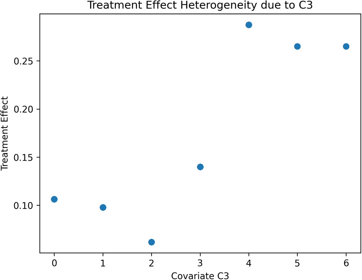
Figure 4. Scenario 1: Scatterplot reporting ATE's heterogeneity values due to Covariate 3 estimated.
In the second simulation, we carried out the same settings as before, with the difference that this time, we simulated an RCT with a continuous treatment X.
In the case of continuous treatment, it is even more evident that the importance of detecting subsets of our sample that might produce divergent outcomes. In Figure 5, we can notice how, in the left terminal node, 16% of our sample had a negative Y value of −.41 in contrast with almost 15% that had a .41 increase in Y.

Figure 5. Scenario 2: Simulation of a causal tree with a continuous treatment (X), one normally distributed covariate (C1) and two non-normally distributed covariates (C2, C3). Max-depth set to 3.
As in the previous scenario, Figures 6–8 report the estimated treatment effects heterogeneity due to different values of covariates C1, C2 and C3 in our Scenario 1 with a binary treatment.

Figure 6. Scenario 2: Scatterplot reporting ATE's heterogeneity values due to Covariate 1 estimated using a causal forest model (2000 trees).
Depending on the distribution of each covariate, such heterogeneity can take different shapes. In the case of C1, a normally distributed variable, C2 has an exponential distribution and C3 follows a normal distribution skewed with a skewness parameter a = 10. The treatment effect can vary even more than in our scenario 1. For example, Figure 6 reports the treatment effect variation conditional to the values of C1 where the spread of the heterogeneity is complex, with a group of cases well above the average, a group on a null effect and a small group with negative values. Figure 7 reports the case of a different type of covariate, C2, which is exponentially distributed, where we can identify from the scatterplot that the treatment effects variation is contained in a range of values of C2, like in Scenario 1. Last, we have Figure 8, the most problematic of all, C3 has a skewed normal distribution, the result is a complex picture with a polarisation of effects for several groups with positive and some with negative treatment effects values.

Figure 7. Scenario 2: Scatterplot reporting ATE's heterogeneity values due to Covariate 2 estimated using a causal forest model (2000 trees).

Figure 8. Scenario 2: Scatterplot reporting ATE's heterogeneity values due to Covariate 3 estimated using a causal forest model (2000 trees).
As shown by these simulations, which only partially simulate real data complexity, the issue of detecting and identifying the heterogeneity of treatment effects conditional to covariates deserves attention and effort. The use of computational methods like causal trees and causal forests to not only detect the heterogeneity but link it to specific cases in our sample produces a new set of rich information. How this information can be used in the context of behavioural science is an open discussion, we will offer one possibility in the next section.
Conclusions
The use of computational methods has started to be applied in the context of behavioural studies, see for example, Steinert Janina et al. (Reference Steinert Janina, Sternberg, Prince, Fasolo, Galizzi Matteo, Büthe and Veltri Giuseppe2022) in the context of testing messages against COVID-19 vaccine hesitancy in a pan-European study. Applications in the private sector are also more and more common, estimation of heterogeneous treatment effects is essential for treatment targeting, which is particularly relevant in the industry when the idea of individualised targeting and treatment is already popular. At the same time, the very same techniques are being applied to observational data (Brand et al., Reference Brand, Xu, Koch and Geraldo2021), where causal estimation based on different methods is increasingly common. From a methodology perspective, the field is continuously evolving, and there are alternatives. For example, an interesting element of innovation is represented by the so-called Metalearners (Künzel et al., Reference Künzel, Sekhon, Bickel and Yu2019). Metalearners are algorithms capable of using different estimation models at the same time. We have seen different estimators introduced by Künzel et al. (Reference Künzel, Sekhon, Bickel and Yu2019) that leverage flexible machine learning algorithms to estimate heterogeneous treatment effects. The estimators differ in their degree of sophistication: the S-learner fits a single estimator including the treatment indicator as a covariate. The T-learner fits two separate estimators for the treatment and control groups. Lastly, the X-learner is an extension of the T-learner that allows for different degrees of flexibility depending on the amount of data available across treatment and control groups. Among the many other papers, it's important to mention the R-learner procedure of Nie and Wager (Reference Nie and Wager2021). Another alternative is using a Bayesian framework, like the Bayesian Additive Regression Trees (BART) (Green and Kern, Reference Green and Kern2012). One of the benefits of using advanced Bayesian models like BART for estimating causal effects is that the posterior provides simultaneous inference on CATEs, sample average treatment effects and everything in between. Moreover, it provides opportunities for summarising the information in the posteriors. Recent developments in applying causal machine learning to heterogeneity analysis include ‘causal clustering’ (Kim, Reference Kim2020; Kim and Zubizarreta, Reference Kim and Zubizarreta2023), which can be used to ascertain subgroups with similar treatment effects, applying clustering techniques to an unknown outcome to be estimated. This represents an intriguing new application of clustering methods that have yet to be exploited in causal inference and the heterogeneous effects problem.
While it is clear that the analytical approach is technically growing fast, it is less obvious how to place it within the context of behavioural research from a more theoretical standpoint. The latter is a discussion that is in its early stages. One possible application is what we can call the ecological use of heterogeneity. This is in line with the recent discussions in the behavioural science community about the need to understand contextuality (Banerjee and Mitra, Reference Banerjee and Mitra2023), to address hidden heterogeneity in a population (Schimmelpfennig et al., Reference Schimmelpfennig, Vogt, Ehret and Efferson2021), to model personalised intervention based on individual models (Krpan et al., Reference Krpan, Makki, Saleh, Brink and Klauznicer2021; Mills, Reference Mills2022).
Identifying heterogeneous treatment effects in behavioural research is functional in identifying what we can call behavioural niches. It is well known that one of the main forces shaping the adaptation process is natural selection. That is, the evolution of organisms can be seen as the result of selective pressure to adapt to their environment. Adaptation is thus seen as a kind of top-down process from the environment to the living creature (Godfrey-Smith, Reference Godfrey-Smith1998). In contrast, several evolutionary biologists have recently attempted to provide an alternative theoretical framework by emphasising the role of niche construction (Odling-Smee et al., Reference Odling-Smee, Laland and Feldman2003). According to this view, the environment is a kind of ‘global marketplace’ offering unlimited possibilities. In fact, not all the possibilities the environment offers can be exploited by human and non-human animals acting upon it. For example, the environment provides organisms with water for swimming, air for flying, flat surfaces for walking, etc. However, no creature is completely capable of exploiting them all. Furthermore, all organisms seek to modify their environment to exploit better the elements that satisfy them and eliminate or mitigate the effects of the negative ones. This environmental selection process allows living creatures to construct and shape ‘ecological niches’. An ecological niche can be defined, following Gibson, as a ‘set of environmental characteristics that are suitable for an animal’ (Gibson, Reference Gibson1979). It differs from the notion of habitat in the sense that niche describes how an organism experiences its environment, whereas habitat simply describes where an organism lives. In each ecological niche, the selective pressure of the local environment is drastically modified by organisms to diminish the negative impacts of all those elements to which they are not adapted. This new perspective constitutes a different interpretation of the traditional theory of evolution, introducing a second system of inheritance called the ecological inheritance system (Odling-Smee et al., Reference Odling-Smee, Laland and Feldman2003).
In other words, one way to compare human populations is regarding the variety of behavioural ecological niches available to individuals as avenues to social or material diversity. This is a similar point made by Schimmelpfennig and Muthukrishna (Reference Schimmelpfennig and Muthukrishna2023) that behavioural science should engage with cultural evolutionary thinking, considering population diversity, among other things. In ecological biogeography, a niche generally describes the fit of a species to particular environmental conditions (Odling-Smee et al., Reference Odling-Smee, Laland and Feldman2003). For our purposes, a niche refers to a particular way of extracting resources from the environment and/or from other individuals and thus is situated with respect to the socioecological features of the local surroundings. Theoretically, niches define a context for doing certain things or behaving in certain ways that penalise or reward given behavioural strategies. Different niches create different payoffs to particular behavioural strategies.
In Figure 9, we tentatively illustrate this point. Whenever we are in mode A of behavioural research, the case of identifying the determinants of a given behaviour or decision-making outcome, the exploitation of these complex methods to identify local variations of our models can enrich us in formulating a more robust version of our final model. In other words, Models 1, 2 and 3 in the diagram will help us to rethink our general model. If we are in case B of Figure 9, the common situation of testing a behavioural intervention, we find ourselves in the context discussed in this paper. One important aspect is the selection of covariates; this topic would require a detailed discussion. However, if we accept the notion of ecological use of these methods, then covariates should be descriptors of socioecological context. If we have such covariates, then the identification of LATE can be treated as evidence of behavioural niches. In other words, the initial and tentative definition of a behavioural niche is the set of LATEs identifying using socioecological covariates. In turn, this could be a starting point to investigate each niche or develop specific interventions tailored to each niche if required. The selection of the socioecological covariates will be theoretical, but their importance will be data-driven if we use the partitioning methods described earlier. In conclusion, in this paper, we have introduced and explained how the application of computational social science methods, namely causal trees and forests, could be beneficial for behavioural research and, perhaps, provide an answer to some of the challenges that this field is currently facing in terms of a more sophisticated investigation of the heterogeneity in treatment effects. Moreover, such methods might open new lines of enquiries and theoretical thinking as outlined by the notion of behavioural niches.

Figure 9. The ecological use of heterogeneity: behavioural niches.


 Open access