


1. Introduction
Why distributional learning?
Very early in life humans master the sound system of their language. A growing number of studies suggest that one of the processes by which infants and adults acquire speech sound contrasts is distributional learning (Escudero, Benders & Wanrooij, Reference Escudero, Benders and Wanrooij2011; Hayes-Harb, Reference Hayes-Harb2007; Kleinschmidt & Jaeger, Reference Kleinschmidt and Jaeger2015; Maye & Gerken, 2001; Ong, Burnham & Escudero, Reference Ong, Burnham and Escudero2015; Wanrooij, Boersma & van Zuijen, Reference Wanrooij, Boersma and van Zuijen2014a). Distributional learning is an unsupervised statistical learning mechanism that works through exposure to the probability distributions of speech sounds in one's environment. In the laboratory, distributional learning is instantiated as a training phase that includes statistical distributions of sounds. A number of studies have shown that learners exhibit the effects of distributional training after only a few minutes of exposure (Maye & Gerken, 2001; Maye, Weiss & Aslin, Reference Maye, Weiss and Aslin2008), while others failed to find the expected effects in some conditions (Ong, Burnham, Escudero & Stevens, Reference Ong, Burnham, Escudero and Stevens2017; Wanrooij, Boersma & van Zuijen, Reference Wanrooij, Boersma and van Zuijen2014b). Whether or not distributional training is effective could depend on the type of participants tested (e.g., infant vs. adults, or learners vs. naïve listeners) but also on the learning scenario at hand (e.g., learning of a new contrast vs. an adaptation of an old one).
Traditional application: category creation
Previous experiments have usually tested whether distributional training leads to the creation of new categories – that is, whether it affects learners’ discrimination of an unfamiliar speech sound contrast. Researchers exposed one group of listeners to a bimodal distribution of sounds and another group to a unimodal distribution (or to a flat distribution, or to music) and many of them found that after several minutes of exposure, the group listening to the bimodal distribution discriminated the contrast more successfully than the other group(s) (e.g., Escudero et al., Reference Escudero, Benders and Wanrooij2011; Maye, Werker, & Gerken, Reference Maye, Werker and Gerken2002); see Figure 1a for an example of bimodal versus unimodal stimulus design typically used in previous studies. For instance, Maye et al. (Reference Maye, Werker and Gerken2002) exposed American English infants to bimodal or unimodal distributions between a pre-voiced [d] and a voiceless unaspirated [t], both of which fall within the same phonemic category /d/ in English. Maye et al. found that bimodally-trained infants could discriminate the non-native contrast better than unimodally-trained infants.
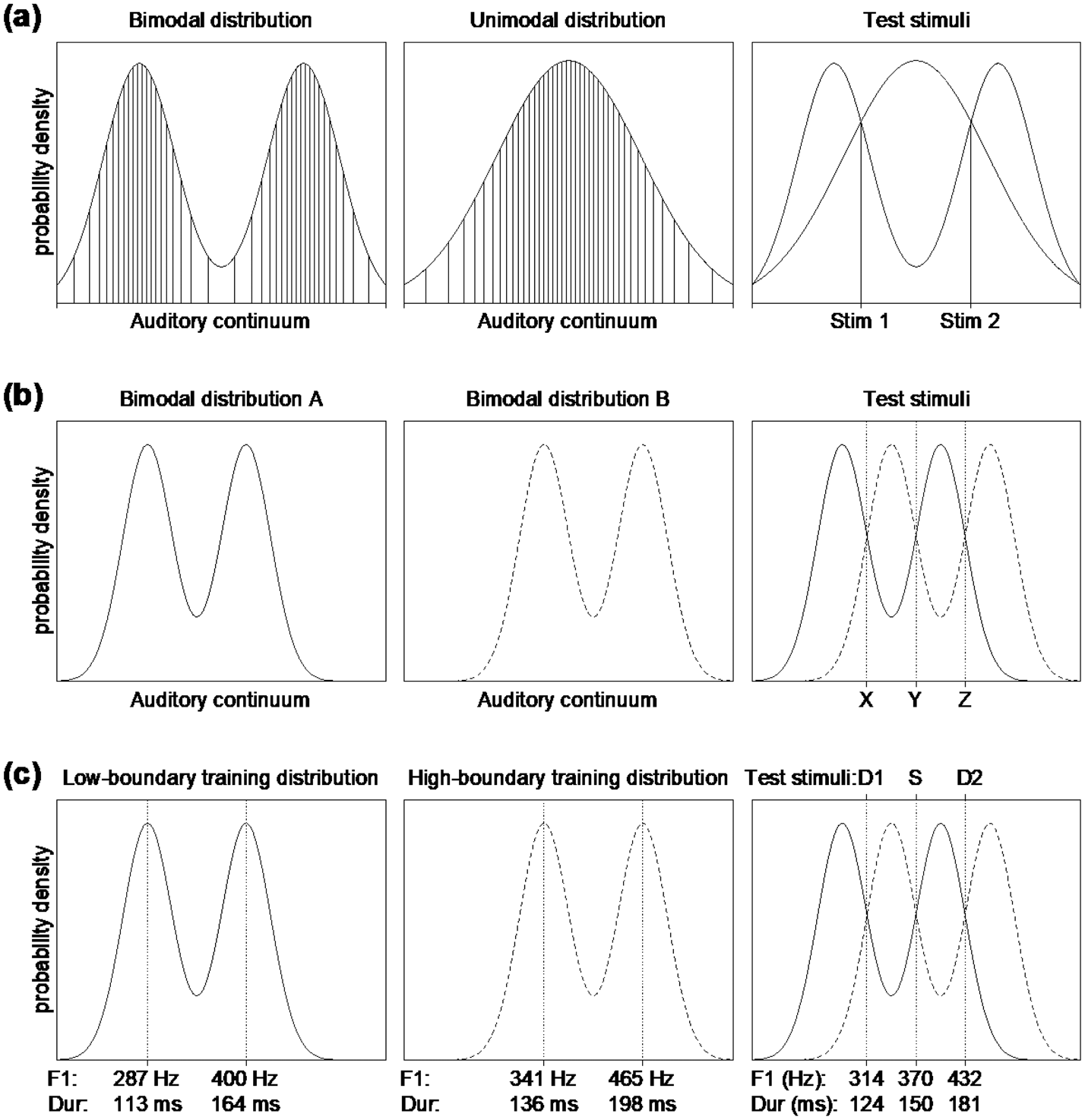
Figure 1. (a) Typical unimodal and bimodal training distributions as used in the distributional training literature. The left and middle graphs show “continuously sampled” bimodal and unimodal training distributions such as those reported in Wanrooij and Boersma (Reference Wanrooij and Boersma2013), where the actual stimuli are represented by the vertical lines. The right graph illustrates the locations of the test stimuli traditionally used to assess the effects of distributional training. (b) Illustration of two bimodal training distributions (left and middle), and three test stimuli (right). The right graph illustrates that under the lowered-boundary distribution (solid curve), test stimuli Y and Z fall within the same peak, whereas test stimulus X falls into the other peak. In contrast, under the raised-boundary distribution (dashed curve), test stimuli X and Y fall within the same peak, whereas test stimulus Z falls into the other peak. (c) The actual training distributions used in the present experiment for the low-boundary (left graph, solid line) and high-boundary (middle graph, dashed line) training groups; for the meaning of D1, S, and D2, see text. The values of peak locations are marked on the x-axis for each training dimension (F1 and duration): top row of marks = F1 values in Hz; bottom row = duration values in ms. The right graph shows the stimuli used in the oddball paradigm in pre- and post-test, and their values in Hz or ms. The x-axis is scaled in ERB for F1 and logarithmically for duration.
Distributional learning has been originally described as the unsupervised learning mechanism that infants employ early in life to acquire the categories for native-language speech sounds (Maye et al., Reference Maye, Werker and Gerken2002). Later studies showed that distributional learning of new speech sound contrasts can occur also in adults, albeit with varying success (Escudero et al., Reference Escudero, Benders and Wanrooij2011; Escudero & Williams, Reference Escudero and Williams2014; Maye & Gerken, Reference Maye, Gerken, Do, Domínguez and Johansen2001; Ong et al., Reference Ong, Burnham and Escudero2015; Pajak & Levy, 2011; Terry, Ong & Escudero, Reference Terry, Ong and Escudero2015; Wanrooij & Boersma, Reference Wanrooij and Boersma2013; Wanrooij, Escudero & Raijmakers, Reference Wanrooij, Escudero and Raijmakers2013; Wanrooij, De Vos & Boersma, Reference Wanrooij, De Vos and Boersma2015a). This seems reasonable: even adult listeners are engaged in some form of perceptual learning on an every-day basis: to successfully communicate with talkers with specific speech idiosyncrasies and accents, as well as in noisy environments, listeners need to continuously adapt their perceptual categories to the ambient talkers and situations, and they may employ distributional learning to achieve this (Kleinschmidt & Jaeger, Reference Kleinschmidt and Jaeger2015).
Another application: boundary adaptation with phoneme labels
Unlike unsupervised category creation in infants, perceptual adaptation of existing categories in adults typically involves some higher-level representations (i.e., top–down supervision): listeners associate an atypical speech sound with the phoneme category that is lexically plausible in a given context. For instance, when hearing a sound midway between a typical [f] and [s], i.e., [f/s], listeners associate it with /s/ if it occurs in a word like glass but with /f/ if it occurs in a word like cliff. As a result, listeners retune, or shift, their perceptual boundary between /f/ and /s/: the boundary is shifted towards [s] if they heard the [f/s] sound in the context for /f/, and vice versa (Eisner & McQueen, Reference Eisner and McQueen2005).
The adaptation of existing category boundaries has been attested in distributional training experiments as well. Clayards, Tanenhaus, Aslin and Jacobs (Reference Clayards, Tanenhaus, Aslin and Jacobs2008) exposed adult speakers of American English to bimodal distributions of sounds that had either narrow or wide peaks. The authors found that differences in the exposed peak widths lead to differences in the crispness of the listeners’ perceptual boundary between /p/ and /b/: listeners exposed to a bimodal distribution with wide peaks had a shallower phoneme boundary than listeners exposed to a bimodal distribution with narrow peaks. Theodore, Monto and Graham (Reference Theodore, Monto and Graham2020) found distributionally-learned boundary crispness adjustments, too, for a /k/-/g/ contrast (furthermore demonstrating that the success of the distributional learning depended on individuals’ receptive language abilities). Kleinschmidt, Raizada and Jaeger (Reference Kleinschmidt, Raizada, Jaeger, Dale, Jennings, Maglio, Matlock, Noelle, Warlaumont and Yoshimi2015) exposed American English listeners to bimodal distributions with a shifted location of the /p/-/b/ boundary and had them perform a word identification task with word-initial [p]s and [b]s drawn from the shifted distributions. Irrespective of whether they received explicit trial-by-trial information on the intended phoneme identity, listeners shifted their /p/-/b/ boundary accordingly. Colby, Clayards and Baum (Reference Colby, Clayards and Baum2018) found that after listening to bimodal /ɪ/-/ɛ/ distributions with an altered boundary, young and older American English-speaking adults can shift their perceptual boundary with as well as without lexical feedback (see also Schreiber, Onishi & Clayards, Reference Schreiber, Onishi and Clayards2013 for an adaptation of the /m/-/n/ boundary). These findings show that listeners can (re-)associate an atypical bimodal sound distribution of sounds with their existing two-way category contrast even if the to-be adapted category is not a priori specified (similar adaptation occurs when training stimuli are non-existent words, Chládková, Podlipský & Chionidou, Reference Chládková, Podlipský and Chionidou2017). Note that although Kleinschmidt et al.'s or Colby et al.'s participants were not necessarily given feedback as to which category of the to-be-shifted contrast an atypical speech sound belonged to, due to the nature of the identification task (during training or during pre-test), the participants did activate and use the two phoneme labels associated with the target two-way contrast. In that sense, the previously documented boundary shift in distributional training was of an implicitly supervised nature.
Novel application: boundary adaptation without phoneme labels
We propose that DT can be used to induce boundary shift without an overt use of phoneme labels. In this study we examine whether boundary shifts occur in an unattended paradigm in which listeners are not required to label nor even attend to the stimuli. Testing whether boundary shift can at all occur entirely pre-attentively, we do not further elaborate on whether the boundary shift reflects short-term perceptual adaptation (specific e.g., to the talker at hand or testing session) or whether it reflects a longer-term restructuring of linguistic categories.
The proposal that a fully unattended distributional training can lead to a (temporary or lasting) boundary shift is put to the test here. We expose participants to probability distributions of stimuli that indicate a displacement of their native-language boundary, and test whether they shift their perceptual boundaries according to the exposed distributional statistics. Boundary shifts can be tested by comparing distributional training across two otherwise identical bimodal distributions that are shifted with respect to each other in the location of their peaks.
How to implement an unattended DT for boundary shift: discrimination with three points
The present experiment involves Spanish-native listeners who are implicitly and pre-attentively trained to shift their native-language perceptual boundary of the /i/–/e/ contrast. These two phonemes differ primarily in their first formant (F1), and to some extent in their second formant (F2), so the auditory continuum along which our distribution varies is based on both F1 and F2. During training, half of the listeners are exposed to a bimodal distribution with a lowered category boundary (i.e., a lowered F1 and a raised F2) as compared to the average location of the /i/–/e/ boundary in their native language; this distribution is schematized in Figure 1b (left). The other listeners are instead exposed to a bimodal distribution with a raised category boundary, as in Figure 1b (middle). It can be seen in the Figure that the peak and valley locations differ between the two training distributions. Traditionally, peaks are thought to represent category centers, and valleys are thought to represent category boundaries.
Figure 1b (right) shows the test stimuli. The location of the test stimuli with respect to the distributions allows for inferences about the intended category membership: for listeners trained with the lowered boundary (solid curve), test stimuli Y and Z should have become instances of the same category, whereas test stimulus X should have become an instance of the other category. In contrast, for listeners trained with the raised boundary (dashed curve), test stimuli X and Y should fall within the same category, whereas Z should fall into the other category. In other words, stimulus Z (or, stimulus D2 in Figure 1c, right) represents a within-category change in the low-boundary training condition but a between-category change in the high-boundary training condition, while stimulus X (or, stimulus D1 in Figure 1c, right) represents a between-category change in the low-boundary training condition but a within-category change in the high-boundary training condition.
Predicted results for boundary shift
If distributional training leads to boundary shifts in adults’ perception, we predict that for the /i/-/e/ contrast the trained boundary location (i.e., the low-boundary distribution or the high-boundary distribution in Figure 1c) will interact with test stimulus (i.e., stimulus D1 or D2 in the Figure). In line with perceptual categorization, the difference between D1 and S should be perceived as larger after low-boundary training (where it represents a between-category difference) than after high-boundary training (where it represents a within-category change), while the difference between D2 and S should be perceived as larger after high-boundary training (where it represents a between-category difference) than after low-boundary training (where it represents a within-category change).
Crucially, whether or not listeners learned from the distributions is tested without requiring them to use their lexical knowledge: we test the extent to which listeners pre-attentively discriminate the three target points on the continuum without having them overtly identify each sound as one or the other category. To minimize any (implicit) interference of higher-level knowledge or overt category labels, we employ an unattended testing paradigm assessing listeners’ perceptual discrimination at the neural level, measuring the brain's mismatch response.
Why the three-point method should be good for category creation as well
The scheme in Figure 1b should work not only for boundary shift, but also for DT's traditional goal of establishing category creation. Spanish listeners, for instance, can be distributionally trained on a non-native contrast between a short /ɪ/ and a long /ɪː/. This is why we tested a second group of twenty native Spanish listeners, exposing half of them to a bimodal distribution along the durational dimension with a shorter duration boundary, as in Figure 1b (left) and the other half to a bimodal distribution with a longer duration boundary, as in Figure 1b (middle), after which they are tested with three durations, as in Figure 1b (right). In fact, if DT is found with our three-points method, this will provide better evidence for the existence of DT than the unimodal-versus-bimodal method of Figure 1a used to do, because the latter method has been criticized for potentially confounding the number of peaks with the widths of the peaks (Wanrooij, Boersma & Benders, Reference Wanrooij, Boersma and Benders2015b), a criticism that cannot apply to the three-point method.
Predicted results for category creation
If DT works for the novel duration contrast, the perceived D2–S difference should be greater for Spanish listeners trained on the high-boundary distribution than for Spanish listeners trained on the low-boundary distribution, and the perceived D1-S difference should be greater for those trained on the low-boundary distribution than for those trained on the high-boundary distribution.
The current design could potentially answer a question about the difference in learning on the spectral (F1/F2) continuum versus on the duration continuum, and/or between boundary shift and category creation. If adults use distributional statistics more effectively for boundary shift (which they have to do all the time in real life) than for category creation (which they probably did for the last time when they were children learning their native language, or when they learned a second language), we predict that the distributional training effect will be larger for a native contrast than for a novel contrast. If we find such a difference for the native /i/–/e/ contrast when compared with the novel short–long contrast, it could be due either to a difference between category shift and category creation, or to a difference between spectrum and duration, or to both, and further research would have to disentangle these causes. The present work provides to the research community at least a potential robust methodology for disentangling these alternative explanations.
Implications for second-language learning theories and findings
The question to what extent second-language (L2) learners can successfully create novel categories/learn to use new phonetic cues, or adapt their first-language (L1) categories/reuse old phonetic cues, has occupied researchers for a long time. While creating a new category along a new dimension has been shown to be easier than splitting a category (Flege, Reference Flege and Strange1995), shifting the boundaries of existing categories appears to be the easiest learning mechanism (Escudero, Reference Escudero, Boersma and Hamann2009; Escudero & Boersma, Reference Escudero and Boersma2004; McAllister, Flege & Piske, Reference McAllister, Flege and Piske2002). To what extent learners are able to reuse familiar phonetic cues in an L2 seems to depend on whether they already have similar, two-way contrasts signaled by this cue in their L1 (Llompart & Reinisch, Reference Llompart and Reinisch2019). Here we test whether the relative ease of reusing familiar categories and cues over novel ones during L2 speech acquisition is measurable in an unattended unsupervised learning experiment.
Leaving aside the variously intricate many-to-one and one-to-many L1-L2 category mappings, our experiment directly speaks to the debate of new versus old cues and categories. Comparing category shift on an old dimension to category creation on a new dimension, we predict that the former will yield larger learning effects than the latter. This prediction is inspired by the findings of several recent studies on phonetic cue-specific or domain-specific learning and adaptation (Schertz, Cho, Lotto & Warner, Reference Schertz, Cho, Lotto and Warner2016; Siegelman, Bogaerts, Elazar, Arciuli & Frost, Reference Siegelman, Bogaerts, Elazar, Arciuli and Frost2018). For instance, Schertz et al. (Reference Schertz, Cho, Lotto and Warner2016) show that when listeners are exposed to conflicting distributions of cues to plosive voicing (namely, F0 and VOT), they downweigh the cue which in their native language is secondary and attend to the distributional information carried by the native-language primary cue. That is, cues that are weighted heavier in the native language could be learnt from better than cues that are less important in the native language. Our prediction is also inspired by L2 phonetic studies showing that L2 learners naturally and easily shift their L1 category boundaries or the weighting of existing L1 acoustic dimensions to match the boundaries and cue-weighting of the same contrast or dimensions in their L2 (e.g., Escudero, Reference Escudero, Boersma and Hamann2009; Yazawa, Whang, Kondo & Escudero, Reference Yazawa, Whang, Kondo and Escudero2020). For instance, Yazawa et al. (Reference Yazawa, Whang, Kondo and Escudero2020) recently showed that Japanese learners of English who use both duration and spectral information for L1 vowel contrasts can modify their cue-weighting for both dimensions from a high reliance on duration for Japanese to a higher reliance on spectral information in their L2 English, matching native American English listeners’ cue weighting for vowel contrasts. In line with this recent research in L1 and L2 listeners, we can thus predict that the cue that is present in our listeners’ phonology (i.e., F1 in Spanish) will be learnt from more readily, and can lead to better L2 acquisition results than a cue that is absent from their phonology (i.e., duration in Spanish).
2 Method
2.1 Participants
Forty native speakers of Spanish took part in the experiment (20 women and 20 men). They were university students, from Spain as well as Latin America, between 19 and 36 years old, with no history of hearing, speech, or neurological disorders. Three additional people were tested, but their data were not further analyzed because of a technical error during recording (2 participants) or noisy EEG data (1 participant with more than 65% of artifact-contaminated epochs). The participants were all functional Spanish monolinguals: they had been raised in a monolingual Spanish-speaking family, and although they had learned English as a second language they rated their proficiency in English as below average (i.e., as 3 or less on scale from 0 to 7). At the time of testing they were either tourists or new international students who arrived in the Netherlands less than 2 weeks prior to the experiment. Their exposure to foreign languages (English and Dutch) was minimal. Before testing, the participants were not familiar with the training purpose of the study. The experiment conformed to the standards of the ethical committee of the Faculty of Humanities, University of Amsterdam, and was conducted after a participant gave a written informed consent.
The participants were randomly assigned to one of two dimension groups, within which they were assigned to one of two boundary groups, as shown in Table 1. That is, 20 participants were trained to shift their native category boundary along an old dimension – namely, vowels’ first formant (F1) – while the other 20 were trained to create categories on a novel dimension – namely, vowel duration. Within each dimension group, 10 participants were trained with a low boundary location and 10 were trained with a high boundary location. The details of training are given in Section 2.2.
Table 1. Predicted discrimination per boundary location, and the division of the 40 participants into the 4 groups, i.e., 2 auditory dimensions times 2 boundary locations.

2.2 Training
During a 9-minute training phase, participants were exposed to a total of 600 acoustically different sounds that were sampled from a bimodal distribution (mixture of two Gaussians with equal variances) along either the F1 or duration dimension, with the equal-area method described by Wanrooij and Boersma (Reference Wanrooij and Boersma2013), and randomly permuted for each participant. The location of the two peaks (the Gaussian means), and the valley separating them, differed between participants: for half of the participants on either dimension, the valley in the bimodal distribution was located in the lower half of the F1 or duration range (low-boundary training group, Fig. 1c left), while for the other half of the participants, the valley was located in the upper half of the F1 or duration range (high-boundary training group, Fig. 1c middle). Section 2.4 provides details about the synthesis and the acoustic values of the stimuli.

Figure 2: The grand average ERPs at FCz of Deviant 1 and Deviant 2 in pre- (black dashed line) and posttest (black solid line), and the posttest-pretest difference (red online, grey in print, solid line), plotted for each training boundary location, and dimension. Shading shows the 100-ms window in which we searched for the grand-peak in the MMN analysis.

Figure 3: The absolute difference waves at FCz for each dimension, training boundary location, and stimulus type. The MMR analysis window is shaded. Note that for the duration dimension, two windows are marked, because the analysis window differed between D1 (earlier window) and D2 (later window), see section 2.6.
The training distributions for the F1 dimension were designed with respect to the average native Spanish perceptual boundary between the vowels /i/ and /e/, which is roughly 370 Hz (see Benders, Escudero & Sjerps, Reference Benders, Escudero and Sjerps2012; Chládková & Escudero, Reference Chládková and Escudero2012; a token from our stimulus set that had an F1 of 370 Hz was judged as most ambiguous between /i/ and /e/ by three native speakers of Spanish). The low-boundary group was trained with a boundary at a lower F1 value (i.e., 341 Hz) than the average native Spanish /i/-/e/ boundary. The high-boundary group was trained with a boundary at a higher F1 value (i.e., 400 Hz) than the average Spanish /i/-/e/ boundary.
For the duration dimension, the training distributions were designed with respect to an average perceptual boundary between short and long vowels in languages that use vowel duration contrastively, which is roughly 150 ms (see Chládková, Escudero & Lipski, Reference Chládková, Escudero and Lipski2013; Meister, Werner & Meister, Reference Meister, Werner and Meister2011). Crucially, 150 ms represents the most ambiguous duration value also in Spanish adult learners of second-language length contrasts (Escudero, Benders & Lipski, Reference Escudero, Benders and Lipski2009; Lipski, Escudero & Benders, Reference Lipski, Escudero and Benders2012). The training-distribution boundaries in the present study were set at 136 ms for the low-boundary training group, and at 164 ms for the high-boundary training group. Figure 1c plots the training distributions with values of their peak locations for F1 and for duration. The boundary locations of the training distributions were shifted by a comparable number of just-noticeable differences for both the F1 and the duration dimension; see section 2.4.
2.3 Pre- and post-test
Discrimination before and after training was measured using event-related potentials – namely, as the unattended mismatch response, recorded using electroencephalography (EEG). The mismatch response is elicited with an oddball paradigm, i.e., with infrequent “deviant” stimuli in a sea of “standard” stimuli. For each dimension, we created an oddball presentation with two deviant types (Deviant 1 and Deviant 2: D1 and D2, amongst standards: S, in Fig. 1c) such that each deviant type occurred 75 times, with a probability of 12.5%. The presentation started with 10 repetitions of the standard, and there were always at least two standards separating one deviant from the following one. In total, there were 610 stimuli (150 deviants and 460 standards) per oddball presentation. The inter-stimulus interval jittered randomly in five steps between 750 and 870 ms. For F1, the Standard had F1 values representative of the Spanish /i/-/e/ boundary, while the two deviants had F1 values typical for Spanish /i/ (Deviant 1) or /e/ (Deviant 2). For duration, the Standard had duration values representative of a perceptual boundary between a short and a long [ɪ]-vowel (non-native), while the two deviants were a short (Deviant 1) and a long (Deviant 2) version of this vowel. The right graph in Figure 1c plots the F1 or duration values of stimuli from pre- and post-test. The acoustic properties of the stimuli are described in detail in Section 2.4.
Per participant we generated one oddball sequence for pre-test and a different oddball sequence for post-test. Each test took about 10 minutes. After the pre-test, participants took a break of 10 to 15 minutes, during which they filled in a questionnaire, had some refreshment, and had a conversation with the experimenter, who was a native speaker of Spanish. The break was followed by training, which was, after a short pause of a few minutes, followed by the post-test.
To assess the genuine effects of the training distribution and dimension at hand, we trained each participant with only one type of training and only on one dimension, instead of having them return e.g., for a second session in which they would be trained with a different boundary or on a different dimension. This between-subjects design ensured that each participant's pre-test corresponded to the initial native Spanish stage as closely as possible.
If listeners learn from the distributions they were exposed to during training (see Section 2.2.), the trained locations should affect listeners’ pre-attentive discrimination of stimuli at post-test. Specifically, for the low-boundary training group, Standard and Deviant 2 should be perceived as one category and Deviant 1 as the other category (the “oddball”), while for the high-boundary training groups, Standard and Deviant 1 should be perceived as one category and Deviant 2 as the oddball (see the right graph in Figure 1c and Table 1).
2.4 Unattended paradigm
The experiment aimed at recreating an unattended learning scenario and eliciting a pre-attentive neural response by implementing the following. Throughout the entire experiment participants watched a self-selected muted movie with subtitles in Spanish: there was thus no overt task, i.e., not even in the pre- and post-test, that would direct their attention to the auditory stimuli. Before the experiment started, they were told to try to enjoy the movie and ignore the sounds that would be played. Additionally, in the breaks between the blocks, the experimenter chatted with the participant about the movie and never about the sound stimuli.
2.5 Stimuli
The sounds from the training as well as the sounds from the pre- and post-test were isolated synthetic vowels. They were made using the Klatt synthesizer in Praat (Boersma & Weenink, Reference Boersma and Weenink1992–2016). The vowels modeled a male voice. They had a falling pitch slope starting at 135 Hz at the beginning of the vowel and ending at 101 Hz. The amplitude was ramped at a 5-ms portion at each vowel edge. The F3 of all vowels was 2750 Hz, F4 was 3400 Hz, F5 was 4050 Hz; to get a flatter spectrum, higher resonating frequencies up to F20 were added with a 1000-Hz step between every two neighboring formants. The F1, F2 and duration of the vowels depended on which training dimension they were part of.
For stimuli from the F1 training, the duration of all vowels was 150 ms. The F1 range between 5.36 ERB and 11.52 ERB (corresponding to 200 Hz and 600 Hz) was sampled into 600 different values according to one of the two bimodal distributions (low-boundary or high-boundary). The low-boundary distribution had means at 7.05 ERB and 8.90 ERB (287 Hz and 400 Hz); the high-boundary distribution had means at 7.98 ERB and 9.83 ERB (341 Hz and 465 Hz). The standard deviation for both peaks (the RMS width) was 0.46 ERB. In order to render the stimuli naturally sounding, the F2 was correlated inversely with the vowels’ F1, ranging between 22.78 ERB and 21.08 ERB (2500 Hz and 2038 Hz). The F1 and F2 of the three stimuli from the F1 test were: 370 Hz and 2255 Hz for the Standard, 314 Hz and 2328 Hz for Deviant 1, and 423 Hz and 2195 Hz for Deviant 2; all other acoustic properties were identical to those of the stimuli from the training. The distance between each two adjacent test stimuli was about 4 to 5 just-noticeable differences (JNDs; see Kewley-Port & Watson, Reference Kewley-Port and Watson1994, who report 13 Hz as the JND for the F1 of /ɪ/-like vowels with American English listeners).
For stimuli from the duration training, the F1 of all vowels was 370 Hz, and the F2 was 2255 Hz. The range of durations between 80 ms and 280 ms (scaled logarithmically) was sampled into 600 different values according to one of the two bimodal distributions. The low-boundary distribution had means at 113 ms and 164 ms; the high-boundary distribution had means at 136 ms and 198 ms. The standard deviation for both peaks was 0.09 along the logarithmic scale (which is approximately 10 ms for the peak at 113 ms, and approximately 18 ms for the peak at 198 ms). The durations of the test stimuli were: 150 ms for the Standard, 124 ms for Deviant 1, and 181 ms for Deviant 2. The distance between each two adjacent test stimuli on the duration dimension was between 4 and 5 JNDs (assuming the JND for duration is approximately 3.75%: see Goudbeek, Swingley & Smits, Reference Goudbeek, Swingley and Smits2009; Smits, Sereno & Jongman, Reference Smits, Sereno and Jongman2006, who respectively report the JND for duration of 5% and 2.5% with Dutch and American English listeners). The perceptual distances between the test stimuli on the duration dimension were thus comparable to the perceptual distances between the test stimuli on the F1 dimension.
2.6 EEG recording and preprocessing
The EEG was recorded from 64 active electrodes placed according to the 10/20 international placement system (BioSemi) and from 7 external channels at the following locations: nose, left and right mastoid, left and right temple, and above and below the right eye. The EEG was recorded at 8kHz and downsampled off-line to 512 Hz. Further EEG processing and ERP analyses were done in the software Praat (Boersma & Weenink, Reference Boersma and Weenink1992-2016). The signal of each electrode was referenced off-line to the nose channel. A drift in the signal was removed by subtracting from each of the nine channels a straight line such that the amplitude at the first and at the last sample of the channel became 0. The signal in each channel was subsequently filtered in the frequency domain with a high-pass filter at 1Hz (bandwidth 0.5 Hz), a low-pass filter at 25 Hz (bandwidth 12.5 Hz), and a notch filter at 50 Hz.
In each channel, the data were segmented into 600-ms epochs running from -100 ms to 500 ms relative to stimulus onset, and baseline-corrected by subtracting the average of the 100-ms pre-stimulus interval. Epochs in which the amplitude at any channel exceeded ±70 μV were removed. The artefact rejection procedure led to the exclusion of 1 participant, as only data of those with at least 65% of artefact-free epochs were included and further analyzed. For each of the remaining 40 participants, the artefact-free epochs were averaged per stimulus type (Standard, Deviant 1, Deviant 2) and test type (pre-test, post-test), yielding 6 curves per channel per participant. The averaged signals of only nine electrodes were selected for further analysis: at three degrees of anteriority – namely, frontal (F), fronto-central (FC) and central (C); and at three degrees of laterality – namely, left (giving electrodes F3, FC3 and C3), right (F4, FC4 and C4) and midline (“zero”: Fz, FCz and Cz). These channels were chosen because they typically reflect strongest auditory mismatch responses.
2.7 MMN analysis
In order to compare physically identical stimuli, we computed one difference wave per deviant type by subtracting the response in pre-test from the response to the same stimulus in post-test, yielding two curves per channel per participant. That is, the average ERP to D1 in pre-test was subtracted from the ERP to D1 in post-test, and analogously, the average ERP to D2 in pre-test was subtracted from the ERP to D2 in post-test. This approach ensures that comparison is done between stimuli that have identical physical properties and that any differential responses result from the different function (here, its category status, supposedly learned during training) that the stimulus had at pre- versus post-test (see Jacobsen & Schröger, Reference Jacobsen and Schröger2003 for detail on why one should compare mismatch responses across physically identical stimuli). In each of the 72 grand-mean difference waveforms (one per combination of deviant type, boundary location, dimension, and channel, each averaged over 10 participants) we searched for a negative peak (“grand peak”) in a 120–220-ms window after deviation onset. For the F1 dimension the analysis window was 120–220 ms after stimulus onset for both deviant types, while for the duration dimension the window was 244–344 ms for the short deviant (Deviant 1; because the earliest possible deviation onset for the short deviant was 124 ms after stimulus onset, i.e., the duration of the short deviant) and 270–370 ms for the long deviant (Deviant 2; because the earliest possible deviation onset for the long deviant was 150 ms after stimulus onset, i.e., the duration of the standard). In the individual participants’ difference waveforms, we centered a shorter 40-ms window at the latency of the grand peak and computed the mean amplitude over the 40-ms window, which we further refer to as the MMN amplitude. Figure 2 plots the grand averaged ERP responses to each deviant in pre- and post-test as well as the post-test minus pre-test difference waves; figures A1–A4 in the Appendix show individual participants’ post-test minus pre-test difference waves for each deviant.
2.8 Absolute MMR analysis
Besides the negative MMN that is usually used in adult ERP literature, we also computed the absolute mismatch response (MMR) as a measure of our participants’ perceptual discrimination of the stimuli. While in adults, the mismatch response typically has a negative polarity, in infants and young children, it often displays a positive polarity; and, as children mature, a negative MMN is observed (Cheng, Wu, Tzeng, Yang, Zhao & Lee, Reference Cheng, Wu, Tzeng, Yang, Zhao and Lee2015; Maurer, Bucher, Brem & Brandeis, Reference Maurer, Bucher, Brem and Brandeis2003). However, in several studies with preschool and school-age children, positive mismatch responses have been observed for some deviant types, and it has been suggested that these reflect immature stages of change detection (Lee, Yen, Yeh, Lin, Cheng, Tzeng & Wu, Reference Lee, Yen, Yeh, Lin, Cheng, Tzeng and Wu2012; Partanen, Torppa, Pykäläinen, Kujala & Huotilainen, Reference Partanen, Torppa, Pykäläinen, Kujala and Huotilainen2013; Shafer, Yu & Datta, Reference Shafer, Yu and Datta2010). The polarity of the mismatch response thus not only indexes the maturation of the neural change-detecting apparatus in general, shifting from positive to negative values throughout lifetime, but it might reflect also the developmental stage of individual phoneme contrasts, being negative for more established categories or phonetic features and positive for the less well established ones (Cheng et al., Reference Cheng, Wu, Tzeng, Yang, Zhao and Lee2015; Lee et al., Reference Lee, Yen, Yeh, Lin, Cheng, Tzeng and Wu2012). The magnitude of the perceived difference between a standard and a deviant can also be reflected as a greater positive or negative (i.e., absolute) deflection for more salient deviants and smaller absolute deflection for less salient ones (Maurer et al., Reference Maurer, Bucher, Brem and Brandeis2003). Despite the co-occurring negative and positive MMR polarities found in childhood, one could speculate that MMR polarity might also vary across the learning stages for novel speech sound contrasts in adulthood. Here besides testing the negative MMN as is typical in ERP experiments with adults, we analyzed the absolute mismatch response, thus combining potential early-stage acquisition effects demonstrated by a small or/and positive deflection as well as more mature-stage effects demonstrated by a larger or/and negative deflection. Note that before training, both the F1 and the duration deviants might represent a non-salient or even non-categorical change: on the F1 dimension both D1 and D2 are initially a within-category change from the Standard boundary-stimulus, and on the durational dimensions they are most probably undefinable with respect to category structures. We thus cannot predict what polarity each deviant's mismatch response could have, and consequently, we cannot predict how it would change with training. What we can predict is that if training enhances categorization and thus also the perceived saliency, the mismatch response (with either positive or negative deflection) at hand will be of a greater magnitude after than before training. This is why we analyze the absolute mismatch response.
From the difference waveform obtained with the subtraction described in Section 2.6, we created an absolute difference waveform by converting each sample's measured amplitude to its absolute value. The absolute difference waveforms are plotted in Figure 3. From the absolute difference waves, we computed the mean absolute MMR amplitude over the entire 120–220-ms post-deviation-onset window (one value for each combination of speaker, channel and deviant type, yielding 720 values in total), by averaging over the time samples within the window. See the previous section, which defines the deviation onset for each dimension and deviant type.
3. Results
The 720 data points (40 participants, 9 channels, 2 deviant types) were analyzed with linear mixed-effects models in R version 3.3.2 (R Core Team, 2016) using the package lme4 version 1.1-12 (Bates, Maechler, Bolker & Walker, Reference Bates, Maechler, Bolker and Walker2015). We ran one model (with lmer, using restricted maximum likelihood) in which the dependent variable was the MMN amplitude (post-test minus pre-test) and one in which the dependent variable was the absolute MMR amplitude (post-test minus pre-test, then its absolute value). Each of the two models contained five fixed effects, all of which had orthogonal sum-to-zero contrasts. The two between-participant predictors were Dimension (with duration coded as –0.5 and F1 as +0.5) and Boundary (with low coded as –0.5 and high as +0.5). The three within-participant predictors were Deviant (with D1 coded as –0.5 and D2 as +0.5), Laterality (with two contrasts – namely, LateralityA with right coded as –0.5 and left as +0.5, and LateralityB with left and right coded as –1/3 and the midline as +2/3), and Anteriority (with two contrasts – namely, AnteriorityA with central coded as –0.5 and frontal as +0.5, and AnteriorityB with frontal and central coded as –1/3 and fronto-central as +2/3). In the maximal model we therefore fitted 72 fixed parameters: the intercept, all seven main effects, all 19 two-way interactions, all 25 three-way interactions, all 16 four-way interactions, and all four five-way interactions. Participant was entered as a random effect, with per participant potentially one random intercept and 13 random slopes – namely, one for each of the five within-participant contrasts and one for each of their eight two-way interactions. However, such a maximal random-effects structure would invariably lead to a singular model, so that we ended up including only 1 random slope per participant, namely for the single within-participant predictor that is involved in our research questions, namely Deviant. The parameters that may be able to answer our research questions (see Table 1 in the Method section) are the two-way Boundary × Deviant interaction and the three-way Dimension × Boundary × Deviant interaction; the other 70 parameters could provide only exploratory results.
As all the predictors are uncorrelated by design (all contrasts are orthogonal, each possible combination of levels of within-participant predictors occurs equally often in each participant's data, and each possible combination of between-participants predictors had the same number of participants), it is natural to work with a maximal model, so as to reduce the unexplained variance (Barr, Levy, Scheepers & Tily, Reference Barr, Levy, Scheepers and Tily2013). After deciding on a model, we are no longer free to try out smaller models (Simmons, Nelson & Simonsohn, Reference Simmons, Nelson and Simonsohn2011). Convergence problems forced us to go with a model that is still maximal in its fixed-effects structure (i.e. it includes all interactions) but is minimal in its random-effects structure in that it includes only the research-question-answering within-participant predictor(s): our research question is answered by a three-way interaction that involves one within-participant predictor (Deviant), so we need random slopes by participant in our model for this predictor in order to be able to generalize the p-value for this three-way interaction to a conclusion for the population. Confidence intervals and p-values are computed with lmerTest::contest (Kuznetsova, Brockhoff & Christensen, Reference Kuznetsova, Brockhoff and Christensen2017) using Satterthwaite's approximation for the number of degrees of freedom. All models that we report on converged without singularities.
Mismatch negativity
The full output of the MMN model is given in Table A1 in the Appendix. For the MMN, the following parameters differed significantly from zero. The intercept was –0.484 μV (t [36.002] = –2.170, 95% CI = −0.936 .. –0.032 μV, p = 0.037), which is the estimated MMN for the zero values of the predictors (as the contrasts sum to zero, this is the estimate of the grand mean MMN). Thus, on average there was indeed a negativity, as expected. The Boundary × Deviant interaction predicted by Table 1 was not significant as a main effect (though it was in the direction expected for a negativity: –0.263 μV, t [35.999] = –0.275, 95% CI = −2.207 .. +1.680 μV, p = 0.79), nor was its interaction with Dimension (+0.329 μV, 95% CI = −3.558 .. +4.216 μV, t [35.999] = +0.172, p = 0.86). We thus turn to the MMR results to see if we can get a clearer picture.
Absolute mismatch response
The full output of the MMR model is shown in Table A2 in the Appendix. For the absolute MMR, the following parameters differed significantly from zero. The intercept was +1.895 μV (t [36.000] = +22.991, 95% CI = +1.728 .. +2.062 μV), which is the estimated absolute MMR for the zero values of the predictors (as the contrasts sum to zero, this is the estimate of the grand mean absolute MMR, as can also be deduced from Table 2 by averaging across the means reported for the individual conditions). The positive and significant intercept shows that overall, the stimuli were processed differently at post-test than at pre-test, most probably reflecting increasing familiarity or perceptual attunement to the testing stimuli. The main effect of Dimension was +0.332 μV (t [36.000] = +2.016, 95% CI = −0.002 .. +0.667 μV, p = 0.051): as confirmed by Table 2, on average, F1 has a 0.332 μV higher absolute MMR than duration, which on its own could be interpreted as a more pronounced overall perceptual tuning for F1 than for duration. The interaction between Boundary and Deviant, which was expected according to Table 1, was not significant, being only +0.458 μV (t [35.999] = +1.138, 95% CI = −0.358 .. +1.275 μV, p = 0.26), which estimates a 0.458/2 = 0.229 μV greater absolute MMR (averaged over F1 and duration) for the average of low-boundary Deviant1 and high-boundary Deviant2 than for the average of high-boundary Deviant1 and low-boundary Deviant2, as is again confirmed by Table 2. However, this null result is qualified by the significant three-way interaction of Dimension × Boundary × Deviant being +2.519 μV (t [35.999] = +3.129, 95% CI = +0.886 .. +4.153 μV, p = 0.0035), which means that the absolute MMR for the average of low-boundary Deviant1 and high-boundary Deviant2 minus the absolute MMR for the average of high-boundary Deviant1 and low-boundary Deviant2 is 2.519/2 = 1.260 μV greater for F1 than for duration, which is the last thing that can be seen from Table 2. In other words, the triple interaction between Dimension, Boundary and Deviant indicates that in the expected direction of the effect displayed in Table 1, the effect is larger for F1 than for duration.
Table 2: The absolute MMR (means and 95% confidence intervals in μV) elicited by D1 and D2 in low and high boundary training groups, for the F1 dimension and for duration.

Exploring the remaining 4 estimated parameters that came with an interpretable t-value (i.e., that did not involve Laterality or Anteriority, the two within-participant predictors for which the model did not include random slopes), we can say that none showed a significant result.
The three-way interaction Dimension × Boundary × Deviant is the only effect we can use to answer our research-question. To locate the Boundary × Deviant effect predicted in Table 1, we consider separate analyses for F1 and for duration (the complete output of these two separate models is reported in the Appendix, Tables A3 and A4). Referenced to F1 (i.e., with F1 recoded as 0 and duration as 1), the Boundary × Deviant interaction becomes +1.718 μV (t [35.999] = +3.017, 95% CI = 0.563 .. 2.873 μV, p = 0.0047), i.e., it lies in the expected direction. Namely, for F1, low-boundary training D1 yielded a larger MMR than D2, and high-boundary training D2 yielded a larger MMR than D1, as predicted by distributional learning and Table 1. Referenced to duration (i.e., with F1 recoded as 1 and duration as 0), the Boundary × Deviant interaction becomes –0.801 μV (t [35.999] = −1.412, 95% CI = −1.956 .. +0.354 μV, p = 0.17), which is nonsignificant (for a direction opposite from the one expected from Table 1). It can be concluded that the expected Boundary × Deviant interaction (i.e., fast distributional learning) is found in the Spanish-speaking population for F1 (p = 0.0047), and that it is greater for F1 than for duration (p = 0.0035), if it exists for duration at all.
4. Discussion
Our findings show that adults can learn from short unattended exposure to statistical distributions of sounds. Spanish adults do so to a larger extent for their native F1 dimension than for the nonnative duration dimension (if they do it at all for that dimension). After unattended exposure to speech sound distributions with shifted peak/valley locations on the F1 dimension, which is familiar from their native language, adult Spanish learners come to shift their perceptual vowel boundaries. Having been played various [i] and [e] sounds drawn from a distribution with a boundary shifted towards [i], listeners assign [i] (but not [e]) to a different category than [ɪ]. In contrast after being played sounds from a distribution with a boundary shifted towards [e], listeners assign [e] (but not [i]) to a different category than [ɪ]. The shift of phoneme boundaries occurs without any feedback or supervision, which confirms that perceptual recalibration might happen without lexical context and without overtly inducing phoneme category labels.
Plausible interpretation
This fast phonetic learning may occur because Spanish listeners are already familiar with the critical dimension from their native language and can thus learn to adjust the parameters of their already-existing categories. Such a fast adjustment of native category properties would align well with previous literature showing that the distributional properties of stimuli presented in a categorization task affect the participants’ perceptual categories. Clayards et al. (Reference Clayards, Tanenhaus, Aslin and Jacobs2008) found that when the variance of the /p/ and /b/ categories was larger, the perceptual boundaries were shallower, and vice versa. Kleinschmidt et al. (Reference Kleinschmidt, Raizada, Jaeger, Dale, Jennings, Maglio, Matlock, Noelle, Warlaumont and Yoshimi2015) showed that when the /p/ and /b/'s distributions were shifted, the perceptual boundary locations were adjusted accordingly.
In considering the category shift along F1 in the present experiment, possibly what mediated it was not only the mere familiarity with F1 as an auditory cue (whose presence could signal a sonorant as opposed to an obstruent, for instance), but also the existence of native perceptual categories contrasted by the value of the F1 cue (as in contrasting multiple vowel heights). While auditory information informed the listeners there are two clusters of sounds in the environment, the information from the native phonology informed them that those two clusters most likely represent a contrast that already exists in their phonology, i.e., the /i/-/e/ distinction. On each trial, an incoming auditory value was unconsciously associated with the learner's existing mental representation of /i/ or /e/. For instance, when a very peripheral (i.e., low-F1) token of /i/ was played, the mental /i/ category was activated and at the same time updated that category's properties to contain slightly lower F1 values as well, which in turn shifted the center of the /i/-category away from its original location, and could in fact already also shift the boundary between this and the neighboring category /e/ toward a lower F1 value. Hearing an atypical token of /e/ in the initial trials (shifted in the similar direction as the peripheral /i/, toward lower F1 values) further pushed the /e/ category and thus reinforced the updating of the /e/–/i/ boundary location. Such an on-line process that updated the category properties at every trial eventually brought about a more or less stabilized readjustment of the perceptual boundary that was reflected in the listeners’ neural response at post-test. Crucially, this mechanism was made possible by the existence of a native contrast along the dimension that the listeners were trained on, albeit without the listeners’ awareness of or overt attention to speech sound labels. Our training and test paradigms were fully unattended, which is a methodological innovation over previous distributional training studies on category shift. Even at such a pre-conscious level, listeners may implicitly activate their mental phoneme representations. If this is indeed what enabled the category shift here, our neural results parallel the results of previous behavioral studies that employed overt categorization tasks during, or before, distributional exposure.
The fact that no native contrast existed for the duration dimension could explain why the learning effects for duration were smaller, if present at all (this might also explain a null result by Ong et al., Reference Ong, Burnham and Escudero2015, who in their unattended condition did not find a learning effect in Australian English listeners exposed to probability distributions of a Thai tone contrast; however, note that the usual caveat against interpretations of nonsignificant p-values applies). The literature on learning across modalities suggests that explicit supervision, or feedback, facilitates distributional learning (Ashby, Queller & Berretty, Reference Ashby, Queller and Berretty1999; Goudbeek, Cutler & Smits, Reference Goudbeek, Cutler and Smits2008). Probably, in order to form new categories via distributional exposure, at least some implicit top-down information flow is needed for fast distributional learning in adults to take place: both lexicon and distributional information may be needed for the emergence of abstract categories (Boersma et al., Reference Boersma, Escudero and Hayes2013; Feldman, Griffiths, Goldwater & Morgan, Reference Feldman, Griffiths, Goldwater and Morgan2013). Recent studies indicate that the mechanism of unsupervised statistical (including distributional) learning may not be readily available for category creation on phonetic dimensions with which listeners have no prior experience (Chládková & Šimáčková, Reference Chládková and Šimáčková2021; Ong et al., Reference Ong, Burnham, Escudero and Stevens2017). Our findings add to that recent literature by showing that category creation on an uncolonized dimension (duration) was smaller (if any) than category shift on a familiar dimension (F1).
Instead of being modulated directly by the lexicon, category creation in distributional training might also be facilitated by incorporating prediction or competition into the learning scenario. Novel tone-accent categories in American English listeners are learnt more accurately in a training design where tone predicts object outcome than vice versa (Nixon, Reference Nixon2018). Relatedly, Olejarczuk, Kapatsinski and Baayen (Reference Olejarczuk, Kapatsinski and Baayen2018) propose an error-driven model of distributional learning whereby more surprising stimuli yield greater learning steps than unsurprising stimuli. Introducing competition, too, leads to successful category formation (McMurray, Aslin & Toscano, Reference McMurray, Aslin and Toscano2009). Note that in ours as well as across previous studies, the amount of distributional exposure in category creation and in category adaptation scenarios was comparable (typically lasting several minutes). Potentially, category creation in adults might simply require more (bottom-up) exposure than category shift. The question which of the above factors most robustly modulate the success of category creation in distributional training is testable and could be addressed in future studies.
A potential confound
Above, we attempted to explain our results by referring to the nativeness of the phonetic dimension. We cannot yet exclude that the boundary shift we found here for F1 is instead language-independent, applying universally to the frequency dimension. On-line sensitivity to distributional information has, after all, been reported even for discrimination of pure tones (i.e., non-speech sounds) at the level of neural processing: Garrido, Teng, Taylor, Rowe and Mattingley (Reference Garrido, Teng, Taylor, Rowe and Mattingley2016) showed that when the stimuli in an oddball paradigm were sampled from a narrow distribution, deviant sounds elicited a larger MMN response than when the stimuli were sampled from a broad distribution; this finding for non-speech sounds parallels the boundary-crispness changes reported for speech sound contrasts by Clayards et al. (Reference Clayards, Tanenhaus, Aslin and Jacobs2008). To be absolutely sure, then, that the difference we found between the F1 and the duration dimension is due to their different status of nativeness, one would have to design an experiment with two continua A and B, with native listeners of a language X that has native contrasts along A but not along B, plus native listeners of a language Y that has native contrasts along B but not along A.
Relevance to L2 acquisition theories
The present study bears relevance to second-language acquisition research. The ease with which L2 speech sounds are acquired is modulated by both category correspondence (that is, to how many L1 categories an L2 sound assimilates) and cue familiarity (that is, whether a dimension distinguishing an L2 contrast also distinguishes L1 contrasts), as well as by their interaction. As for cue familiarity, it has been debated whether speech sound learning in a second language is easier for new dimensions that are unused by the native language phonology or whether it is easier for old dimensions which are used to differentiate a similar native speech sound contrast (see e.g., Bohn, Reference Bohn and Strange1995; McAllister et al., Reference McAllister, Flege and Piske2002). Our findings that distributional training had the expected effects for the old, F1 dimension, speak in favor of the latter, as did the results reported by Goudbeek et al. (Reference Goudbeek, Cutler and Smits2008). Furthermore, the finding that listeners promptly adjusted their boundary for a contrast that already exists in their native language supports the proposal formulated by Escudero and Boersma (Reference Escudero and Boersma2004) and Escudero (Reference Escudero2005; ch 4–7, see also van Leussen & Escudero, Reference van Leussen and Escudero2015 and Yazawa et al., Reference Yazawa, Whang, Kondo and Escudero2020) stating that in L2 acquisition, non-native contrasts are easier to learn when participants only have to shift an already existing native contrast, than when they have to create an entirely new contrast. In the present study, the comparison was made between learners who had to create a new contrast on a new dimension and learners who had to shift an already existing contrast on an old dimension, while in Goudbeek et al. (Reference Goudbeek, Cutler and Smits2008) it was the learning of new contrasts that was compared on both the new and the old dimension. Combining ours and previous findings, it appears that novel speech sound contrasts are easier to acquire when the learner can reuse a phonetic cue which is familiar from their language (either to create a contrast defined by that cue, or to shift an already existing contrast, see also Schertz et al., Reference Schertz, Cho, Lotto and Warner2016), than when they have to start using an entirely new unfamiliar phonetic dimension.
The present finding that native speakers of Spanish were more readily able to shift an /i/-/e/ boundary than to create an /ɪ/-/ɪː/ contrast might, at first, appear surprising if one considers previous studies showing that native Spanish learners of English and Dutch (at least in initial stages of L2 learning) notoriously overrely on duration to distinguish word pairs like the English feel vs. fill or the Dutch maan “moon” vs. man “man” (Escudero & Boersma, Reference Escudero and Boersma2004; Escudero et al., Reference Escudero, Benders and Lipski2009; Kondaurova & Francis, Reference Kondaurova and Francis2008; Lipski et al., Reference Lipski, Escudero and Benders2012; Wanrooij et al., Reference Wanrooij, Escudero and Raijmakers2013). Crucially, the L2 English learning scenario is, however, different from the learning scenario in the present study: in the L2 English case, learners are from the beginning exposed to a combined spectral and durational contrast /iː/-/ɪ/, whereas in the present experiment the target contrast is durational only, i.e., /ɪː/-/ɪ/. Prior work has argued that it is precisely the combination of spectral and durational information that native Spanish speakers rely on in the initial stages of L2 English learning (Morrison, Reference Morrison2008). The present finding that native Spanish speakers showed evidence of learning on the existing spectral dimension but not so much on the novel durational dimension further suggests that a successful creation of a category or a contrast on a novel dimension might require bootstrapping from a familiar dimension.
An interesting avenue for future distributional training research would be to directly compare how category shifting and creation take place along a familiar dimension (for instance, comparing the high-boundary shift of the Spanish /i/-/e/ boundary to a creation of a third [ɛ]-like category on the F1 dimension). In that respect, a recent experiment suggests that category shifting is possible for both an easy and a difficult second-language contrast, though with a varying success: Llompart and Reinisch (Reference Llompart and Reinisch2019) exposed German learners of English to shifted bimodal distributions of English /i/-/ɪ/ in sheep-ship and /ɛ/-/æ/ in bet-bat and found that the learners could in principle adapt their perceptual categorization of both vowel contrasts. Additionally, the adaptation of /ɛ/-/æ/ varied between individuals and was more accurate for those learners who performed better on a word-decision task with the same vowels. These findings suggest that in intermediate-to-advanced L2 learners distributional learning is possible for an L2 contrast which does not exist in their L1 but is cued by a familiar dimension. To what extent distributional learning of novel contrasts on familiar dimensions could work in beginning learners of the L2 who need to create the L2 category(ies) in the first place, and under which conditions, remains to be shown.
A potential limitation to our interpretation in terms of L2 learning is that we do not know to which extent the Spanish listeners treated the isolated vowel stimuli as linguistic and to which extent our experiment mimicked a language learning scenario. The distributions of /e/ and /i/ tokens were in any case atypical for Spanish. The listeners may have treated them as a different language, as an unfamiliar accent of Spanish they have not heard before, or as an atypical speaker of their own accent. We found that they shifted their perceptual boundaries after exposure, which means their brains noticed the atypical situation and adapted to it. Quite likely, it is thus an adaptation situation that underlies a boundary shift, and the difference between adaptation to new speakers, new accents, or new languages may as well be a continuum and perhaps supported by the same learning mechanism. Irrespective of whether the listeners knowingly recognized the /e/-/i/ training distributions as atypical distributions of their native vowel contrast, arguably it was the existence of this native contrast in their phonological lexicon that facilitated perceptual learning from exposure.
The absolute mismatch response (MMR) as a measure of learning
The present study tested phoneme (boundary) learning in adult participants. No effects of distributional training were detected when the negative deflection of the ERP difference waveforms was considered. Learning effects were detected when the mismatch response was measured as the absolute, i.e., polarity-unspecified, deflection of the ERP difference waves. Previous research with infants and children evidences polarity variations in the mismatch response (MMR) conditioned by an individual's neural maturation as well as by a phoneme-specific developmental stage. Our detection of learning effects for the polarity-unspecified MMR suggests that mismatch response reversals in polarity could index a stage of non-native phoneme learning in adults as well. Future studies with adults could test whether and at which learning stage MMR polarities for non-native and native contrasts resemble one another. Data-driven post-hoc observation of our data suggests another possible cause for the positive MMR in some cases: in our presentation paradigm the two deviant stimuli deviated from the standard in opposing directions, which is what could – very speculatively – bring along opposing polarities of the MMR. The effects of deviant directionality on MMR polarity are worth pursuing in future experiments.
Methodological innovation: the three-point paradigm for distributional training
Besides answering our main research question of whether distributional training leads to the shift of phonetic dimensions, our study contributes methodological refinement to the distributional training literature. Many studies found that distributional training has effects on speech sound discrimination in infants and adults. However, some studies did not find the effect, or found it only for some of their participant groups. For instance, the research of Wanrooij and colleagues (Reference Wanrooij, Boersma and van Zuijen2014a, Reference Wanrooij, Boersma and van Zuijen2014b, Reference Wanrooij, De Vos and Boersma2015a) shows that distributional training of the English /æ/–/ɛ/ contrast works much better for Dutch infants than for Dutch adults. Note, however, that Wanrooij and colleagues, as well as many other studies that claimed to have found the expected effects of distributional training, compared a group of subjects trained with a bimodal distribution to a group of subjects trained with a unimodal distribution. Whenever the bimodal group outperformed the unimodal group in their post-training discrimination of the target sounds, the result was traditionally attributed to the difference in the number of peaks in the two groups’ training distributions.
The traditional interpretation of distributional training results was challenged by Wanrooij et al. (Reference Wanrooij, Boersma and Benders2015b) who argued that the effects of distributional learning observed in the literature may not be due to the differences in the number of peaks between a bimodal and a unimodal distribution but may be due to differences in dispersion (width of the distributional peak), which had always been larger for a bimodal than for unimodal distribution. Wanrooij et al. (Reference Wanrooij, Boersma and Benders2015b) reported an experiment where the unimodal and bimodal training distributions had equal dispersions, and demonstrated, with a Bayesian analysis, that after exposure there was no difference between unimodally and bimodally trained participants in their discrimination of the target sounds. The authors concluded that the number of peaks cannot explain the effects observed in the distributional training literature.
The present study avoids the dispersion problem (similarly to some other previous studies testing boundary shift with more coarsely sampled training stimuli, Llompart & Reinisch, Reference Llompart and Reinisch2019; Munson, Reference Munson2011). We do not compare groups with different number of peaks and different dispersions: in our design all training distributions have two peaks and the same dispersion, and it is only the peak (or, valley) locations that differ between our experimental groups. Therefore, we provide a further test to the learning mechanism underlying distributional learning because any effect of training distributions found in the present study can only be attributable to peak/valley locations, disregarding dispersion differences as a possible cause for the results. Our study has thus shown that listeners exploit at least some properties of the peaks in the distributions to which they are exposed.
5. Conclusion
If we play an ingeniously crafted set of speech sounds to adult listeners, we can make them alter the way they listen to sounds of their native language. In our experiment, Spanish listeners came to interpret a sound midway between their native vowels /i/ and /e/ either as /i/ or as /e/, depending on the set of sounds we had exposed them to. We assessed this “boundary shift” effect at the level of pre-conscious speech processing, by measuring the brain's surprise response between 120 and 220 milliseconds after each sound starts to play. While perceptual learning did occur between the language's already existing vowels /i/ and /e/, the same procedure turned out to be less capable (if at all capable) of creating a new boundary on the language's virgin continuum between short and long vowels; our preliminary interpretation of this is that it may be easier to shift an existing contrast than to create a new contrast.
We contributed a methodological innovation over the usual two-point distributional training paradigm, which compares a distribution with one broad peak with a distribution with two narrow peaks. Our three-point distributional training paradigm manages to avoid the confound between peak width and the number of peaks, and could therefore replace several kinds of distributional training paradigms.
Acknowledgements
This work has been supported by the Netherlands Organization for Scientific Research (NWO) grant 277-70-008 awarded to PB, NWO grant 446-14-012, Czech Science Foundation grant 18-01799S, and Charles University grant Primus/17/HUM/19 awarded to KC, and Australian Research Council Future Fellowship FT160100514 awarded to PE. The authors would like to thank Dirk Jan Vet for technical support and Karin Wanrooij for pointing out some of the relevant literature.
Supplementary Material
For supplementary material accompanying this paper, visit https://doi.org/10.1017/S1366728922000086


 Open access