


1 Introduction
There are numerous works aiming at sharp geometric bounds on the mixing time of a finite Markov chain. Examples include Morris and Peres’ evolving sets bound [Reference Morris and Peres39], expressed in terms of the expansion profile, and the related bound by Fountoulakis and Reed [Reference Fountoulakis and Reed19]. The sharpest geometric bounds on the uniform (a.k.a. $L_{\infty }$
) mixing time are given in terms of the log-Sobolev constant (see [Reference Diaconis and Saloff-Coste16] for a survey on the topic) and the spectral profile bound, due to Goel et al. [Reference Goel, Montenegro and Tetali20]. Both determine the uniform mixing time up to a multiplicative factor of order
$L_{\infty }$
) mixing time are given in terms of the log-Sobolev constant (see [Reference Diaconis and Saloff-Coste16] for a survey on the topic) and the spectral profile bound, due to Goel et al. [Reference Goel, Montenegro and Tetali20]. Both determine the uniform mixing time up to a multiplicative factor of order $\log \log [ 1/\min \pi (x)] $
, where throughout
$\log \log [ 1/\min \pi (x)] $
, where throughout $\pi $
denotes the stationary distribution (see [Reference Diaconis and Saloff-Coste16, Reference Kozma32]). The reader is not familiar with mixing time definitions can find them in Section 2.2. Other notions and definitions used below can be found in Sections 1.5 and 1.7.
$\pi $
denotes the stationary distribution (see [Reference Diaconis and Saloff-Coste16, Reference Kozma32]). The reader is not familiar with mixing time definitions can find them in Section 2.2. Other notions and definitions used below can be found in Sections 1.5 and 1.7.
This type of geometric bounds on mixing times are robust under bounded perturbations of the edge weights, and in the bounded degree setup, also under quasi-isometries. That is, changing some of the edge weights by at most some multiplicative constant factor can change these geometric bounds only by some corresponding constant factor. A natural question, with obvious implications to the potential sharpness of such geometric bounds, is whether mixing times are themselves robust under small changes to the geometry of the Markov chain. For instance, can bounded perturbations of the edge weights change the mixing time by more than a constant factor? Similarly, how far apart can the mixing times of simple random walks (SRWs) on two quasi-isometric graphs of bounded degree be? Different variants of this question were asked by various authors such as Pittet and Saloff-Coste [Reference Pittet and Saloff-Coste42, Section 6], Diaconis and Saloff-Coste [Reference Diaconis and Saloff-Coste16, p. 720], and Aldous and Fill [Reference Aldous and Fill3, Open Problem 8.23].
Ding and Peres [Reference Ding and Peres17] constructed a sequence of bounded degree graphs satisfying that the order of the total variation mixing times strictly increases as a result of a certain sequence of bounded perturbations of the edge weights.Footnote 1 In [Reference Hermon24], a similar example is constructed in which the uniform mixing time is sensitive under bounded perturbations of the edge weights, as well as under a quasi-isometry. All these examples are based on the “perturbed tree” example of T. Lyons [Reference Lyons37] (simplified by Benjamini [Reference Benjamini7]). In particular, they are highly non-transitive, and a priori it appears as if what makes such examples work could not be imitated by a transitive example. It remained an open problem to determine whether the total variation mixing time of random walk on vertex-transitive graphs is robust under small perturbations. This was asked by Ding and Peres [Reference Ding and Peres17, Question 1.4] (see also [Reference Kozma32, p. 3] and [Reference Pittet and Saloff-Coste42, Section 6]). In this paper, we give a negative answer to this question, even when the small perturbation preserves transitivity.
We denote the group of permutations of n elements by $\mathfrak {S}_n$
. Recall that a transposition is an element of
$\mathfrak {S}_n$
. Recall that a transposition is an element of $\mathfrak {S}_n$
which exchanges two values and keeps all the rest fixed.
$\mathfrak {S}_n$
which exchanges two values and keeps all the rest fixed.
Theorem 1.1 There exist a pair of sequences of sets of transpositions $S_n$
and
$S_n$
and $S_n'$
such that the Cayley graphs
$S_n'$
such that the Cayley graphs $\operatorname {\mathrm {Cay}}(\mathfrak {S}_{n},S_n)$
and
$\operatorname {\mathrm {Cay}}(\mathfrak {S}_{n},S_n)$
and $\operatorname {\mathrm {Cay}}(\mathfrak {S}_{n},S_n')$
are
$\operatorname {\mathrm {Cay}}(\mathfrak {S}_{n},S_n')$
are $(3,0)$
-quasi-isometric and
$(3,0)$
-quasi-isometric and
 $$\begin{align*}t_{\mathrm{mix}}(\operatorname{\mathrm{Cay}}(\mathfrak{S}_{n},S_n')) \gtrsim t_{\mathrm{mix}}(\operatorname{\mathrm{Cay}}(\mathfrak{S}_{n},S_{n})) \log \log \log |\mathfrak{S}_{n}|. \end{align*}$$
Further, $S_n \subset S_n' \subset S_n^3:=\{xyz:x,y,z \in S_n \}$
.
$S_n \subset S_n' \subset S_n^3:=\{xyz:x,y,z \in S_n \}$
.
Of course, $\log \log \log |\mathfrak {S}_{n}|\asymp \log \log n$
. We formulated the theorem in this way because the size of the group is the more natural object in this context. Let us remark that probably the ratio of mixing time in our example is indeed
$\log \log \log |\mathfrak {S}_{n}|\asymp \log \log n$
. We formulated the theorem in this way because the size of the group is the more natural object in this context. Let us remark that probably the ratio of mixing time in our example is indeed $\asymp \log \log \log |\mathfrak {S}_{n}|$
, but for brevity, we prove only the lower bound.
$\asymp \log \log \log |\mathfrak {S}_{n}|$
, but for brevity, we prove only the lower bound.
The mixing times in Theorem 1.1 are the total variation ones. In what comes, whenever we write mixing time without mentioning the metric, it is always the total variation mixing time. The behavior described in Theorem 1.1 cannot occur for the uniform mixing times which in the transitive setup is quasi-isometry invariant (see Theorem 2.5).
1.1 Variations on a theme
A related question, asked by Itai Benjamini (private communication) is whether there exists some absolute constant $C>0$
such that for every finite group G for all two symmetric sets of generators S and
$C>0$
such that for every finite group G for all two symmetric sets of generators S and $S'$
such that
$S'$
such that $S \subset S'$
we have that the mixing time of SRW on the Cayley graph of G with respect to
$S \subset S'$
we have that the mixing time of SRW on the Cayley graph of G with respect to $S'$
is at most
$S'$
is at most $C \frac {|S'|}{|S|} $
times the mixing time of SRW on the Cayley graph of G with respect to S (a set S is called symmetric if
$C \frac {|S'|}{|S|} $
times the mixing time of SRW on the Cayley graph of G with respect to S (a set S is called symmetric if
![]() ). Our example also disproves this. In fact,
). Our example also disproves this. In fact, $S \subset S' \subseteq S^3$
and
$S \subset S' \subseteq S^3$
and $|S'|-|S| \le \sqrt { |S|}$
, where
$|S'|-|S| \le \sqrt { |S|}$
, where
![]() for
for $i \in \mathbb {N}$
. The definition of an
$i \in \mathbb {N}$
. The definition of an $(a,b)$
-quasi-isometry (see Section 1.5) gives that if
$(a,b)$
-quasi-isometry (see Section 1.5) gives that if $S \subseteq S' \subseteq S^i$
then
$S \subseteq S' \subseteq S^i$
then $\operatorname {\mathrm {Cay}}(G,S)$
and
$\operatorname {\mathrm {Cay}}(G,S)$
and $\operatorname {\mathrm {Cay}}(G,S')$
are
$\operatorname {\mathrm {Cay}}(G,S')$
are $(i,0)$
-quasi-isometric.
$(i,0)$
-quasi-isometric.
The reason that $|S'|-|S|\le \sqrt {|S|}$
is explained in the proof sketch section below—both share a complete graph on some set K with
$|S'|-|S|\le \sqrt {|S|}$
is explained in the proof sketch section below—both share a complete graph on some set K with $|K|\asymp n$
. Hence, this complete graph has an order of
$|K|\asymp n$
. Hence, this complete graph has an order of $\asymp n^2$
edges, and there are only
$\asymp n^2$
edges, and there are only $o(n)$
additional edges. We could have increased
$o(n)$
additional edges. We could have increased $S_n$
by including in it all
$S_n$
by including in it all $|K|!$
permutation of the elements in K, while keeping
$|K|!$
permutation of the elements in K, while keeping $S_n' \setminus S_n$
the same set (of size
$S_n' \setminus S_n$
the same set (of size $o(n)$
), thus making
$o(n)$
), thus making $\frac { |S_{n}'|-|S_n|}{|S_n|} $
tremendously smaller.
$\frac { |S_{n}'|-|S_n|}{|S_n|} $
tremendously smaller.
We will also be interested in weighted versions of the problem, as these allow us to define “weak” perturbations in a natural way. Let $\Gamma $
be a group, and let
$\Gamma $
be a group, and let
![]() be symmetric weights (i.e.,
be symmetric weights (i.e., $w(s)=w(s^{-1})$
) such that the support of W generates
$w(s)=w(s^{-1})$
) such that the support of W generates $\Gamma $
. The discrete-time lazy random walk on
$\Gamma $
. The discrete-time lazy random walk on $\Gamma $
with respect to W is the process with transition probabilities
$\Gamma $
with respect to W is the process with transition probabilities $P(g,g)=1/2$
and
$P(g,g)=1/2$
and $P(g,gs)=\frac {w(s)}{2\sum _{r \in S}w(r)}$
for all
$P(g,gs)=\frac {w(s)}{2\sum _{r \in S}w(r)}$
for all $g,s \in \Gamma $
. We denote its TV (total variation) mixing time by
$g,s \in \Gamma $
. We denote its TV (total variation) mixing time by $t_{\mathrm {mix}}(\operatorname {\mathrm {Cay}}(\Gamma ,W))$
. In continuous time, let
$t_{\mathrm {mix}}(\operatorname {\mathrm {Cay}}(\Gamma ,W))$
. In continuous time, let
![]() be symmetric rates. The continuous-time random walk on
be symmetric rates. The continuous-time random walk on $\Gamma $
with respect to R is the process that has infinitesimal transitions rates
$\Gamma $
with respect to R is the process that has infinitesimal transitions rates $r(s)$
between g and
$r(s)$
between g and $gs$
for all
$gs$
for all $g,s \in \Gamma $
. Denote its mixing time by
$g,s \in \Gamma $
. Denote its mixing time by $t_{\mathrm {mix}}(\operatorname {\mathrm {Cay}}(\Gamma ,R))$
. As in the unweighted case, due to the group symmetry the invariant distribution is uniform and the TV distance between it and the distribution of the walk at some given time is independent of the initial state.
$t_{\mathrm {mix}}(\operatorname {\mathrm {Cay}}(\Gamma ,R))$
. As in the unweighted case, due to the group symmetry the invariant distribution is uniform and the TV distance between it and the distribution of the walk at some given time is independent of the initial state.
Recall that $\mathfrak {S}_n$
is the symmetric group (the group of permutations of n elements). The following is the promised weighted version of our main result.
$\mathfrak {S}_n$
is the symmetric group (the group of permutations of n elements). The following is the promised weighted version of our main result.
Theorem 1.2 For every $f: \mathbb {N} \to [1,\infty )$
satisfying that
$f: \mathbb {N} \to [1,\infty )$
satisfying that $1 \ll f(n) \le \log \log \log n$
, there exist a sequence
$1 \ll f(n) \le \log \log \log n$
, there exist a sequence $(S_n)_{n =3}^{\infty }$
of sets of transpositions
$(S_n)_{n =3}^{\infty }$
of sets of transpositions $S_n\subset \mathfrak {S}_{n}$
and a sequence of weights
$S_n\subset \mathfrak {S}_{n}$
and a sequence of weights $(W_n)_{n=3}^{\infty }$
, such that
$(W_n)_{n=3}^{\infty }$
, such that $W_n=(w_n(s))$
is supported on
$W_n=(w_n(s))$
is supported on $S_n$
and satisfies that
$S_n$
and satisfies that $1 \le w_{n}(s) \le 1+\left (f(n!)/\log \log n\right )^{1/4}$
for all
$1 \le w_{n}(s) \le 1+\left (f(n!)/\log \log n\right )^{1/4}$
for all $s \in S_n$
, and such that
$s \in S_n$
, and such that
 $$ \begin{align} t_{\mathrm{mix}}(\operatorname{\mathrm{Cay}}(\mathfrak{S}_{n},W_n)) \gtrsim t_{\mathrm{mix}}(\operatorname{\mathrm{Cay}}(\mathfrak{S}_{n},S_{n}))f(n!). \end{align} $$
Similarly, in continuous time, if we set $R_{n}=W_n$
(for the above
$R_{n}=W_n$
(for the above $W_n$
), we get that
$W_n$
), we get that
 $$ \begin{align} t_{\mathrm{mix}}(\operatorname{\mathrm{Cay}}(\mathfrak{S}_{n},R_n)) \gtrsim t_{\mathrm{mix}}(\operatorname{\mathrm{Cay}}(\mathfrak{S}_{n},S_{n}))f(n!). \end{align} $$
We remark that the power $1/4$
is not optimal (it was not a priority for us to optimize it). As before,
$1/4$
is not optimal (it was not a priority for us to optimize it). As before, $|S_n|\asymp n^2$
.
$|S_n|\asymp n^2$
.
1.2 A non-transitive example
Our third result shows that if one is willing to consider non-transitive instances, then indeed one can have a bounded degree example whose (usual worst-case) mixing time is of strictly smaller order than the mixing time starting from the best initial state (i.e., the one from which the walk mixes fastest) after a small perturbation. In all previous constructions of graphs with a sensitive mixing time, there was a large set that starting from it, the walk mixes rapidly both before and after the perturbation, and the mixing time is governed by the hitting time of this set (which is sensitive by construction). In particular, the mixing time started from the best initial state is not sensitive.
Let G be a connected graph. Let $W=(w(e):e \in E(G))$
be positive edge weights. Consider the lazy random walk
$W=(w(e):e \in E(G))$
be positive edge weights. Consider the lazy random walk $(X_k)_{k=0}^\infty $
on
$(X_k)_{k=0}^\infty $
on $G,$
i.e., the process with transition probabilities
$G,$
i.e., the process with transition probabilities $P(x,y)=\frac {w(xy)}{2\sum _{z}w(xz)} $
and
$P(x,y)=\frac {w(xy)}{2\sum _{z}w(xz)} $
and $P(x,x)=\frac {1}{2}$
for all neighboring
$P(x,x)=\frac {1}{2}$
for all neighboring $x,y \in G$
. For
$x,y \in G$
. For $x \in G,$
we define the mixing time starting from x by
$x \in G,$
we define the mixing time starting from x by
With this definition, the usual mixing time $t_{\mathrm {mix}}(G,W)$
(see Section 2.2) is equal to
$t_{\mathrm {mix}}(G,W)$
(see Section 2.2) is equal to $\max _xt_{\mathrm {mix}}(G,W,x)$
.
$\max _xt_{\mathrm {mix}}(G,W,x)$
.
Theorem 1.3 There exist a sequence of finite graphs $L_n=(V_n,E_n)$
of diverging sizes and uniformly bounded degree (i.e.,
$L_n=(V_n,E_n)$
of diverging sizes and uniformly bounded degree (i.e., $\sup _n \max _{v \in V_n}\deg v<\infty $
) and a sequence of some symmetric edge weights
$\sup _n \max _{v \in V_n}\deg v<\infty $
) and a sequence of some symmetric edge weights $W_n=(w_n(e):e \in E_{n})$
such that
$W_n=(w_n(e):e \in E_{n})$
such that $1 \le w_{n}(e) \le 1+\delta _n$
for all
$1 \le w_{n}(e) \le 1+\delta _n$
for all $e \in E_{n}$
and such that
$e \in E_{n}$
and such that
 $$ \begin{align} \max_{x\in V_n}t_{\mathrm{mix}}(L_{n},1,x) \le \delta_n \min_{x \in V_n} t_{\mathrm{mix}}(L_{n},W_n,x) \end{align} $$
for some $\delta _n\to 0$
.
$\delta _n\to 0$
.
It follows from Theorem 1.3 that the average TV mixing time, by which, we mean $\inf \{t:\sum _{x}\pi (x)\|{\mathbb P}_x(X_t = \cdot )-\pi \|_{\mathrm {TV}} \le 1/4 \}$
, can be sensitive to perturbations. This is in contrast with the average
$\inf \{t:\sum _{x}\pi (x)\|{\mathbb P}_x(X_t = \cdot )-\pi \|_{\mathrm {TV}} \le 1/4 \}$
, can be sensitive to perturbations. This is in contrast with the average $L_2$
mixing time (see Section 2.2). This gives a negative answer to a question of Addario-Berry (private communication).
$L_2$
mixing time (see Section 2.2). This gives a negative answer to a question of Addario-Berry (private communication).
As in Theorem 1.1, the change in the order of the mixing time in Theorem 1.3 (the inverse of the $\delta _n$
in (1.3)) is
$\delta _n$
in (1.3)) is $o(\log \log \log |V_{n} |)$
. If we replace the condition
$o(\log \log \log |V_{n} |)$
. If we replace the condition $w_n\le 1+\delta _n$
with
$w_n\le 1+\delta _n$
with $w_n\le 1+c,$
then the change in the order of the mixing time can be as large as
$w_n\le 1+c,$
then the change in the order of the mixing time can be as large as $\log \log \log |V_{n} |$
.
$\log \log \log |V_{n} |$
.
Let us quickly sketch the construction of Theorem 1.3 (full details are in Section 4). Let n be some number, and let $S_n$
be the set of transpositions from Theorem 1.2. Let H be a large, fast mixing graph, and let A be some subset of the vertices of H with
$S_n$
be the set of transpositions from Theorem 1.2. Let H be a large, fast mixing graph, and let A be some subset of the vertices of H with $|A|=|S_n|$
and with the vertices of A far apart from one another. The graph L of Theorem 3 has as its vertex set
$|A|=|S_n|$
and with the vertices of A far apart from one another. The graph L of Theorem 3 has as its vertex set $\mathfrak {S}_n\times H$
(we are using here the same notation for the graph and its set of vertices). We choose the edges of L such that random walk on L has the following behavior. Its H projection is just SRW on the graph H. Its
$\mathfrak {S}_n\times H$
(we are using here the same notation for the graph and its set of vertices). We choose the edges of L such that random walk on L has the following behavior. Its H projection is just SRW on the graph H. Its $\mathfrak {S}_n$
projection is also SRW on
$\mathfrak {S}_n$
projection is also SRW on $\operatorname {\mathrm {Cay}}(\mathfrak {S}_n,S_n)$
, but slowed down significantly. Any given transposition
$\operatorname {\mathrm {Cay}}(\mathfrak {S}_n,S_n)$
, but slowed down significantly. Any given transposition $s\in S_n$
can be applied only when a corresponding vertex of A is reached in the second coordinate. The perturbation goes by perturbing only the
$s\in S_n$
can be applied only when a corresponding vertex of A is reached in the second coordinate. The perturbation goes by perturbing only the $\mathfrak {S}_n$
projection. We defer all other details to Section 4.
$\mathfrak {S}_n$
projection. We defer all other details to Section 4.
1.3 A proof sketch
We will now sketch the proof of our main result, Theorem 1.1 (the proof of Theorem 1.2 is very similar). Readers who intend to read the full proof can safely skip this section.
Random walk on $\operatorname {\mathrm {Cay}}(\mathfrak {S}_{n},S_n)$
with
$\operatorname {\mathrm {Cay}}(\mathfrak {S}_{n},S_n)$
with $S_n$
composed of transpositions is identical to the interchange process on the graph G which has n vertices and
$S_n$
composed of transpositions is identical to the interchange process on the graph G which has n vertices and $\{x,y\}$
is an edge of G if and only if the transposition
$\{x,y\}$
is an edge of G if and only if the transposition $(x,y)\in S_n$
. Hence, we need to construct two graphs G and
$(x,y)\in S_n$
. Hence, we need to construct two graphs G and $G'$
on n vertices, estimate the mixing time of the two interchange processes and show that the corresponding Cayley graphs are quasi-isometric.
$G'$
on n vertices, estimate the mixing time of the two interchange processes and show that the corresponding Cayley graphs are quasi-isometric.
Our two graphs have the form of “gadget plus complete graph.” Namely, there is a relatively small part of the graph D which we nickname “the gadget” and all vertices in $G\setminus D$
are connected between them. While D and the corresponding
$G\setminus D$
are connected between them. While D and the corresponding $D'$
in
$D'$
in $G'$
will be small (we will have
$G'$
will be small (we will have $|D|=|D'|$
), they dominate the mixing time of the interchange process.
$|D|=|D'|$
), they dominate the mixing time of the interchange process.
To describe the gadget, let $u\in {\mathbb N}$
and
$u\in {\mathbb N}$
and $\epsilon \in (0,\frac 12)$
be some parameters. The gadget will have u “stages”
$\epsilon \in (0,\frac 12)$
be some parameters. The gadget will have u “stages” $H_1,\dotsc ,H_u$
(the gadget is almost
$H_1,\dotsc ,H_u$
(the gadget is almost $\cup _{i=1}^u H_i$
but not quite). We obtain each
$\cup _{i=1}^u H_i$
but not quite). We obtain each $H_i$
by “stretching” the edges of some graph
$H_i$
by “stretching” the edges of some graph $H_i'$
which is a union of binary trees of depth
$H_i'$
which is a union of binary trees of depth
![]() (note that
(note that $H_i'$
has the depth exponential in i and hence has volume doubly exponential in i). To get
$H_i'$
has the depth exponential in i and hence has volume doubly exponential in i). To get $H_i$
, replace each edge of
$H_i$
, replace each edge of $H_i'$
with a path of length
$H_i'$
with a path of length
![]() . Namely, for each edge
. Namely, for each edge $\{x,y\}$
of
$\{x,y\}$
of $H_i'$
, we add
$H_i'$
, we add $\ell _i-1$
new vertices (denote them by
$\ell _i-1$
new vertices (denote them by $v_1,\dotsc ,v_{\ell _i-1}$
, and denote also
$v_1,\dotsc ,v_{\ell _i-1}$
, and denote also $v_0=x$
and
$v_0=x$
and $v_{\ell _i}=y$
) and connect
$v_{\ell _i}=y$
) and connect $v_j$
to
$v_j$
to $v_{j+1}$
for all
$v_{j+1}$
for all $j\in \{0,\dotsc ,\ell _i-1\}$
; and remove the edge
$j\in \{0,\dotsc ,\ell _i-1\}$
; and remove the edge $\{x,y\}$
.
$\{x,y\}$
.
We still need to explain how many trees are in each $H_i$
and how they are connected to one another and to the rest of the graph. For this, we need the parameter
$H_i$
and how they are connected to one another and to the rest of the graph. For this, we need the parameter $\epsilon $
, which at this point can be thought of as a sufficiently small constant. For each of the vertices in each of the trees (before stretching), we label the children arbitrarily “left” and “right.” For each leaf
$\epsilon $
, which at this point can be thought of as a sufficiently small constant. For each of the vertices in each of the trees (before stretching), we label the children arbitrarily “left” and “right.” For each leaf $x\in H_i$
, we define
$x\in H_i$
, we define $g(x)$
to be the number of left turns in the (unique) path from the root to x. We now let
$g(x)$
to be the number of left turns in the (unique) path from the root to x. We now let
The sets $B_i$
are used twice. First, we use them to decide how many trees will be in each
$B_i$
are used twice. First, we use them to decide how many trees will be in each $H_i$
. For
$H_i$
. For $i=1,$
we let
$i=1,$
we let $H_1$
be one tree. For every
$H_1$
be one tree. For every $i>1$
, we let
$i>1$
, we let $H_i$
have
$H_i$
have $|B_{i-1}|$
trees, and identify each point of
$|B_{i-1}|$
trees, and identify each point of $B_{i-1}$
with one of the roots of one of the trees in
$B_{i-1}$
with one of the roots of one of the trees in $H_i$
. Second, we use the
$H_i$
. Second, we use the $B_i$
to connect the
$B_i$
to connect the $H_i$
to the complete graph. Every leaf of
$H_i$
to the complete graph. Every leaf of $H_i$
which is not in
$H_i$
which is not in $B_i$
is identified with a vertex of the complete graph (the complete graph K will be of size
$B_i$
is identified with a vertex of the complete graph (the complete graph K will be of size $n-o(n)$
, much larger than
$n-o(n)$
, much larger than $\cup _{i=1}^u H_i$
which will be of size
$\cup _{i=1}^u H_i$
which will be of size $O(n^{1/4})$
, and so most of the vertices of K are not identified with a vertex of the gadget). This terminates the construction of G (see Figure 1). Experts will clearly notice that this is a variation on the perturbed tree idea. In other words, while the perturbed tree itself (as noted above) is highly non-transitive, one can use it as a basis for transitive example by examining the interchange process on it.
$O(n^{1/4})$
, and so most of the vertices of K are not identified with a vertex of the gadget). This terminates the construction of G (see Figure 1). Experts will clearly notice that this is a variation on the perturbed tree idea. In other words, while the perturbed tree itself (as noted above) is highly non-transitive, one can use it as a basis for transitive example by examining the interchange process on it.

Figure 1: The gadget. Vertices marked with small squares actually belong to the complete graph rather than to the gadget.
The graph $G'$
is almost identical, the only difference is that in each path corresponding to a left turn we add short bridges. Namely, examine one such path and denote its vertices
$G'$
is almost identical, the only difference is that in each path corresponding to a left turn we add short bridges. Namely, examine one such path and denote its vertices $v_0,\dotsc ,v_{\ell _i}$
as above. Then in
$v_0,\dotsc ,v_{\ell _i}$
as above. Then in $G',$
we add edges between
$G',$
we add edges between $v_{2j}$
and
$v_{2j}$
and $v_{2j+2}$
for all
$v_{2j+2}$
for all $j\in \{0,\dotsc ,\ell _i/2-1\}$
.
$j\in \{0,\dotsc ,\ell _i/2-1\}$
.
Why this choice of parameters? It is motivated by a heuristic that for such graphs, namely, a gadget connected to a large complete graph, the mixing time of the interchange process is the time all particles have left the gadget (they do not have to all be outside the gadget at the same time, it is enough that each particle left the gadget at least once by this time). See Section 1.4 for some context for this heuristic. Thus, we are constructing our $H_i$
such that the time that it takes all particles to leave
$H_i$
such that the time that it takes all particles to leave $H_i$
is approximately independent of i. Indeed, the time a particle takes to traverse a single stretched edge is approximately
$H_i$
is approximately independent of i. Indeed, the time a particle takes to traverse a single stretched edge is approximately $\ell _i^2 \asymp 4^{u-i}$
while each tree of
$\ell _i^2 \asymp 4^{u-i}$
while each tree of $H_i$
has depth
$H_i$
has depth $4^{i-1}u$
(in the sense that this is the depth of the tree before its edges have been stretched) and the particle has to traverse all levels of
$4^{i-1}u$
(in the sense that this is the depth of the tree before its edges have been stretched) and the particle has to traverse all levels of $H_i$
, so it exits
$H_i$
, so it exits $H_i$
after time approximately
$H_i$
after time approximately $4^{u-1}u$
, which is independent of i. And this holds for all particles simultaneously because the probability that a particle takes
$4^{u-1}u$
, which is independent of i. And this holds for all particles simultaneously because the probability that a particle takes $\lambda \cdot 4^{u-1}u$
time to traverse the tree (for some
$\lambda \cdot 4^{u-1}u$
time to traverse the tree (for some $\lambda>1$
) is exponentially small in the number of layers
$\lambda>1$
) is exponentially small in the number of layers $4^{i-1}u$
, and hence that would not happen to any of the particles in the tree, which has approximately
$4^{i-1}u$
, and hence that would not happen to any of the particles in the tree, which has approximately $2^{4^{i-1}u}$
particles, if
$2^{4^{i-1}u}$
particles, if $\lambda $
is sufficiently large. In the roughest possible terms, the growing height of the trees is dictated by the growing number of vertices (which must grow because
$\lambda $
is sufficiently large. In the roughest possible terms, the growing height of the trees is dictated by the growing number of vertices (which must grow because $H_i$
has many more roots than
$H_i$
has many more roots than $H_{i-1}$
, since each
$H_{i-1}$
, since each $x\in B_{i-1}$
is a root of
$x\in B_{i-1}$
is a root of $H_i$
) while the decreasing stretching balances the growing height to get approximately uniform expected exit time. The only exception is
$H_i$
) while the decreasing stretching balances the growing height to get approximately uniform expected exit time. The only exception is $H_1$
, whose height is not dictated by the number of roots (clearly, as there is only one), but by the stretching.
$H_1$
, whose height is not dictated by the number of roots (clearly, as there is only one), but by the stretching.
With the definitions of G and $G'$
done, estimating the mixing times is relatively routine, so we make only two remarks in this quick sketch. How do we translate the fact that all particles visited the complete graph into an upper bound on the mixing time? We use a coupling argument. We couple two instances
$G'$
done, estimating the mixing times is relatively routine, so we make only two remarks in this quick sketch. How do we translate the fact that all particles visited the complete graph into an upper bound on the mixing time? We use a coupling argument. We couple two instances $\sigma $
and
$\sigma $
and $\sigma '$
of the interchange process (in continuous time) using the same clocks and letting them walk identically unless
$\sigma '$
of the interchange process (in continuous time) using the same clocks and letting them walk identically unless $\sigma (x)=\sigma '(y)$
for an edge
$\sigma (x)=\sigma '(y)$
for an edge $\{x,y\}$
that is about to ring, in which case we apply the transposition to exactly one of
$\{x,y\}$
that is about to ring, in which case we apply the transposition to exactly one of $\sigma $
or
$\sigma $
or $\sigma '$
, reducing the number of disagreements (this coupling involves a standard trick of doubling the rates, and censoring each step with probability 1/2). The fact that the complete graph is much larger and has many more edges simplifies our analysis (the reader can find the details of the coupling in Section 3.2).
$\sigma '$
, reducing the number of disagreements (this coupling involves a standard trick of doubling the rates, and censoring each step with probability 1/2). The fact that the complete graph is much larger and has many more edges simplifies our analysis (the reader can find the details of the coupling in Section 3.2).
The lower bound for the mixing time on $G'$
uses the standard observation that adding those edges between
$G'$
uses the standard observation that adding those edges between $v_{2j}$
and
$v_{2j}$
and $v_{2j+2}$
makes the left turn more likely to be taken than the right turns, transforming
$v_{2j+2}$
makes the left turn more likely to be taken than the right turns, transforming $B_i$
from an atypical set (with respect to the hitting distribution of the leaf set of
$B_i$
from an atypical set (with respect to the hitting distribution of the leaf set of $H_i$
) to a typical one, and hence, the particle that started at the root of
$H_i$
) to a typical one, and hence, the particle that started at the root of $H_1$
has high probability to traverse all
$H_1$
has high probability to traverse all $H_i$
before entering the complete graph for the first time. This, of course, takes it
$H_i$
before entering the complete graph for the first time. This, of course, takes it $4^{u-1}u^2$
time units (compare to the mixing time bound of
$4^{u-1}u^2$
time units (compare to the mixing time bound of $4^{u-1}u$
for the interchange process on G). Of course, the mixing time of the interchange process on
$4^{u-1}u$
for the interchange process on G). Of course, the mixing time of the interchange process on $G'$
is also bounded by the time that all particles leave the gadget, but we found no way to use this. We simply bound the time a single particle leaves the gadget and get our estimate.
$G'$
is also bounded by the time that all particles leave the gadget, but we found no way to use this. We simply bound the time a single particle leaves the gadget and get our estimate.
1.4 The mixing time of the interchange process
Since our proof revolves around estimating the mixing time of the interchange process on some graph, let us spend some time on a general discussion of this topic. We first mention some conjectures relating the mixing time of the interchange process on a finite graph G to that of $|G|$
independent random walks on G.
$|G|$
independent random walks on G.
Given a finite graph $G=(V,E)$
and edge rates
$G=(V,E)$
and edge rates $R,$
the corresponding n-fold product chain is the continuous-time Markov chain on
$R,$
the corresponding n-fold product chain is the continuous-time Markov chain on $V^n$
satisfying that each coordinate evolves independently as a random walk on G with edge rates R. This is a continuous-time walk on the n-fold Cartesian product of G with itself, whose symmetric edge rates
$V^n$
satisfying that each coordinate evolves independently as a random walk on G with edge rates R. This is a continuous-time walk on the n-fold Cartesian product of G with itself, whose symmetric edge rates $R_n$
are given by
$R_n$
are given by
 $$\begin{align*}R_n((v_1,\dotsc,v_n),(v_1,\dotsc,v_{k-1},v_k',v_{k+1},\dotsc,v_n)):=R(v_k,v_k') \end{align*}$$
for all $v_1,\ldots ,v_n,v_k' \in V$
and
$v_1,\ldots ,v_n,v_k' \in V$
and $k \in [n]$
. We shall refer to this Markov chain as n independent random walks on G with edge rates R and denote its (TV) mixing time by
$k \in [n]$
. We shall refer to this Markov chain as n independent random walks on G with edge rates R and denote its (TV) mixing time by $ t_{\mathrm {mix}}(n \text { independent RWs on } G,R)$
. As usual, the mixing time is defined with respect to the worst starting tuple of n points, which turns out to be when they all start from the worst point for a single walk on G with edge rates R.
$ t_{\mathrm {mix}}(n \text { independent RWs on } G,R)$
. As usual, the mixing time is defined with respect to the worst starting tuple of n points, which turns out to be when they all start from the worst point for a single walk on G with edge rates R.
Oliveira [Reference Oliveira40] conjectured that there exists an absolute constant $C>0$
such that the TV mixing time of the interchange process on an n-vertex graph G with rates R, i.e.,
$C>0$
such that the TV mixing time of the interchange process on an n-vertex graph G with rates R, i.e., $t_{\mathrm {mix}}(\operatorname {\mathrm {Cay}}(\mathfrak {S}_n,R))$
, is at most
$t_{\mathrm {mix}}(\operatorname {\mathrm {Cay}}(\mathfrak {S}_n,R))$
, is at most $C t_{\mathrm {mix}}(n \text { independent RWs on }G,R)$
. See [Reference Hermon and Salez30, Conjecture 2] and [Reference Hermon and Pymar29, Question 1.12] for two different strengthened versions of this conjecture. See [Reference Hermon and Salez30] for a positive answer for high dimensional products.
$C t_{\mathrm {mix}}(n \text { independent RWs on }G,R)$
. See [Reference Hermon and Salez30, Conjecture 2] and [Reference Hermon and Pymar29, Question 1.12] for two different strengthened versions of this conjecture. See [Reference Hermon and Salez30] for a positive answer for high dimensional products.
For the related exclusion process, some progress on Oliveira’s conjecture is made in [Reference Hermon and Pymar29]. Returning to the interchange process, in the same paper, the following more refined question is asked [Reference Hermon and Pymar29, Question 1.12]: Is $t_{\mathrm {mix}}(\operatorname {\mathrm {Cay}}(\mathfrak {S}_n,R))$
equal up to some universal constants to the mixing time of n independent random walks on
$t_{\mathrm {mix}}(\operatorname {\mathrm {Cay}}(\mathfrak {S}_n,R))$
equal up to some universal constants to the mixing time of n independent random walks on $(G,R)$
starting from n distinct locations? (see [Reference Hermon and Pymar29] for precise definitions). We see that our result is related to finding some graphs G such that the mixing time of
$(G,R)$
starting from n distinct locations? (see [Reference Hermon and Pymar29] for precise definitions). We see that our result is related to finding some graphs G such that the mixing time of $|G|$
independent SRW with edge rates
$|G|$
independent SRW with edge rates $1$
on G, starting from distinct initial locations, is sensitive under small perturbations. In fact, the graphs we construct in this paper satisfy this property too, but in the interest of brevity, we will not prove this claim (the proof is very similar to the one for the interchange process we do provide). This conjectured relation between the exclusion process and independent random walks is behind the heuristic we employed (and mentioned in Section 1.3) to construct our example.
$1$
on G, starting from distinct initial locations, is sensitive under small perturbations. In fact, the graphs we construct in this paper satisfy this property too, but in the interest of brevity, we will not prove this claim (the proof is very similar to the one for the interchange process we do provide). This conjectured relation between the exclusion process and independent random walks is behind the heuristic we employed (and mentioned in Section 1.3) to construct our example.
As we now explain, if we did not require the initial locations to be distinct (as is the case in Oliveira’s conjecture) such sensitivity could not occur. It is easy to show (e.g., [Reference Hermon and Pymar29]) that when $|G|=n,$
 $$\begin{align*}\frac 14 t_{\mathrm{rel}}(G,R) \log n \le t_{\mathrm{mix}}(n \text{ independent RWs on }G,R) \le 4 t_{\mathrm{rel}}(G,R) \log n , \end{align*}$$
where $t_{\mathrm {rel}}(G,R)$
is the relaxation time of
$t_{\mathrm {rel}}(G,R)$
is the relaxation time of $(G,R)$
, defined as the inverse of the second smallest eigenvalue of
$(G,R)$
, defined as the inverse of the second smallest eigenvalue of $-\mathcal {L}$
, where
$-\mathcal {L}$
, where $\mathcal L$
is the infinitesimal Markov generator of the walk
$\mathcal L$
is the infinitesimal Markov generator of the walk $(G,R)$
. The relaxation time is robust under small perturbations (see Section 2.1), and hence so is
$(G,R)$
. The relaxation time is robust under small perturbations (see Section 2.1), and hence so is $ t_{\mathrm {mix}}(n \text { independent RWs on }G,R)$
. Our result that the mixing time is sensitive does not contradict Oliveira’s conjecture, as he conjectured only an upper bound (which, in our case, is sharp for neither
$ t_{\mathrm {mix}}(n \text { independent RWs on }G,R)$
. Our result that the mixing time is sensitive does not contradict Oliveira’s conjecture, as he conjectured only an upper bound (which, in our case, is sharp for neither $S_n$
nor
$S_n$
nor $S_n'$
).
$S_n'$
).
Loosely speaking, in order to make the mixing time of n independent random walks starting at distinct locations of smaller order than (the robust quantity) $t_{\mathrm {rel}}(G,R) \log n$
it is necessary that the eigenvector corresponding to the minimal eigenvalue of
$t_{\mathrm {rel}}(G,R) \log n$
it is necessary that the eigenvector corresponding to the minimal eigenvalue of $-\mathcal L$
be localized on a set of cardinality
$-\mathcal L$
be localized on a set of cardinality $n^{o(1)}$
. This is a crucial observation in tuning the parameters in our construction, which explains why for smaller areas of the graph (namely,
$n^{o(1)}$
. This is a crucial observation in tuning the parameters in our construction, which explains why for smaller areas of the graph (namely, $H_i$
with small index i) we “stretch” edges by a larger factor. This is the opposite of what is done in [Reference Hermon24].
$H_i$
with small index i) we “stretch” edges by a larger factor. This is the opposite of what is done in [Reference Hermon24].
Lastly, we comment that in contrast with a single random walk, in order to change the mixing time of n independent random walks, starting from n distinct initial locations, it does not suffice for the perturbation only to change the typical behavior of the walk, but rather it is necessary that it significantly changes the probabilities of some events in some sufficiently strong quantitative manner. See [Reference Hermon24] for a related discussion, about why it is much harder to construct an example where the uniform mixing time is sensitive than it is to construct one where the TV mixing time is sensitive.
1.5 Quasi-isometries and robustness
Since we hope this note will be of interest to both group theory and Markov chain experts, let us take this opportunity to compare two similar notions related to comparison of the geometry of two graphs or of two reversible Markov chains. The first is the notion of quasi-isometry which is more geometric in nature. The second is the notion of robustness which is more analytic. In particular, we are interested in properties which are preserved by these notions.
This discussion is an important part of the background, but let us advise the readers that it is not necessary to appreciate our results, as they apply in both cases. For example, Theorem 1.1 shows that the mixing time is neither quasi-isometry invariant nor robust.
A quasi-isometry (defined first in [Reference Gromov23]) between two metric spaces X and Y is a map $\phi :X\to Y$
such that for some numbers
$\phi :X\to Y$
such that for some numbers $(a,b)$
we have
$(a,b)$
we have
 $$\begin{align*}\forall u,v\in X \qquad \frac{d(u,v)-b}{a}\le d(\phi(u),\phi(v))\le ad(u,v)+b, \end{align*}$$
where d denotes the distance (in X or in Y, as appropriate). Further, we require that, for every $y\in Y,$
there is some
$y\in Y,$
there is some $x\in X$
such that
$x\in X$
such that $d(\phi (x),y)\le a+b$
. We say that X and Y are
$d(\phi (x),y)\le a+b$
. We say that X and Y are $(a,b)$
quasi-isometric if such a
$(a,b)$
quasi-isometric if such a $\phi $
exists. (Our choice of definition is unfortunately only partially symmetric. If
$\phi $
exists. (Our choice of definition is unfortunately only partially symmetric. If $\phi :X\to Y$
is an
$\phi :X\to Y$
is an $(a,b)$
quasi-isometry then one may construct a quasi-isometry
$(a,b)$
quasi-isometry then one may construct a quasi-isometry $\psi :Y\to X$
with the same a but perhaps with a larger b.)
$\psi :Y\to X$
with the same a but perhaps with a larger b.)
For a property of random walk that is defined naturally on infinite graphs, we say that it is quasi-isometrically invariant if whenever G and H are two quasi-isometric infinite graphs, the property holds for G if and only if it holds for H (the graphs are made into metric spaces with the graph distance). Examples include a heat kernel on-diagonal upper bound of polynomial type [Reference Carlen, Kusuoka and Stroock12], an off-diagonal upper bound [Reference Grigor’yan21], and a corresponding lower bound [Reference Boutayeb10, Reference Grigor’yan, Hu, Lau, Bandt, Zähle and Mörters22]. A particularly famous example is the Harnack inequality [Reference Barlow and Murugan5]. For a quantitative property of random walk naturally defined on finite graphs, such as the mixing time, one says that it is invariant to quasi-isometries if, whenever G and H are $(a,b)$
-quasi-isometric, the property may change by a constant that depends only on a and b and not on other parameters. Similar notions may be defined for Brownian motion on Riemannian manifolds, and one may even ask questions like “if a manifold M is quasi-isometric to a graph G and Brownian motion on M satisfies some property, does random walk on G satisfy an equivalent property?” and a number of examples of this behavior are known.
$(a,b)$
-quasi-isometric, the property may change by a constant that depends only on a and b and not on other parameters. Similar notions may be defined for Brownian motion on Riemannian manifolds, and one may even ask questions like “if a manifold M is quasi-isometric to a graph G and Brownian motion on M satisfies some property, does random walk on G satisfy an equivalent property?” and a number of examples of this behavior are known.
The notion of robustness does not have a standard definition, and in particular, the definitions in [Reference Ding and Peres17] and [Reference Hermon24] differ (and also differ from the definition we will use in this paper). Nevertheless, they all have a common thread: a definition for Markov chains that implies that the property in question is preserved under quasi-isometry of graphs of bounded degree, but that makes sense also without any a priori bound on the transition probabilities. Here, we will use the following definition. Let $\mathcal M$
be the set of finite state Markov chains. We say that a
$\mathcal M$
be the set of finite state Markov chains. We say that a $q:\mathcal M\to [0,\infty ]$
is robust if, for any
$q:\mathcal M\to [0,\infty ]$
is robust if, for any $A \in (0,1], $
there exists some
$A \in (0,1], $
there exists some $K \in (0,1] $
such that the following holds. Assume M and
$K \in (0,1] $
such that the following holds. Assume M and $M'$
are two irreducible reversible Markov chains on the same finite state space V with stationary distributions
$M'$
are two irreducible reversible Markov chains on the same finite state space V with stationary distributions $\pi $
and
$\pi $
and $\pi '$
and transition matrices P and
$\pi '$
and transition matrices P and $P'$
satisfying
$P'$
satisfying
 $$ \begin{align} \begin{aligned} \forall \, x &\in V,& A\pi'(x) &\le \pi(x)\le \tfrac1A\pi'(x), \\ \forall \, f &\in \mathbb{R}^V,& A\mathcal{E'}(f,f)&\le \mathcal{E}(f,f)\le \tfrac1A\mathcal{E'}(f,f), \end{aligned} \end{align} $$
where $\mathcal {E}(f,f)$
and
$\mathcal {E}(f,f)$
and $\mathcal {E}'(f,f)$
are the corresponding Dirichlet forms, namely,
$\mathcal {E}'(f,f)$
are the corresponding Dirichlet forms, namely,
and similarly for $\mathcal {E}'$
. Then
$\mathcal {E}'$
. Then $q(M)\ge Kq(M')$
.
$q(M)\ge Kq(M')$
.
We also define robustness for Markov chains in continuous time, and in this case, we replace $P(u,v)$
above with
$P(u,v)$
above with $\mathcal L(u,v$
) which is the infinitesimal rate of transition from u to v, but otherwise the definition remains the same.
$\mathcal L(u,v$
) which is the infinitesimal rate of transition from u to v, but otherwise the definition remains the same.
If P and $P'$
are SRWs on
$P'$
are SRWs on $(a,b)$
quasi-isometric graphs with the same vertex set (with the quasi-isometry being the identity), whose maximal degrees are at most D, then (1.5) holds with some A depending only on
$(a,b)$
quasi-isometric graphs with the same vertex set (with the quasi-isometry being the identity), whose maximal degrees are at most D, then (1.5) holds with some A depending only on $(a,b,D)$
[Reference Diaconis and Saloff-Coste14]. Thus, a robust quantity is also quasi-isometry invariant between graphs of bounded degree on the same vertex set.
$(a,b,D)$
[Reference Diaconis and Saloff-Coste14]. Thus, a robust quantity is also quasi-isometry invariant between graphs of bounded degree on the same vertex set.
Each notion has its advantages and disadvantages relative to the other notion. Quasi-isometry has the flexibility that the spaces compared need not be identical or even of the same type, indeed the fact that a Lie group (a continuous metric space, indeed a manifold) is quasi-isometric to any cocompact lattice of it (a discrete metric space) plays an important role in group theory. Robustness has the advantage that unbounded degrees are handled seamlessly.
Returning to our results, since the examples of our Theorem 1.1 are not of bounded degree, it is natural to ask if they satisfy a comparison of Dirichlet form of the form (1.5). In fact, this is true because in said examples our pair of sets of generators $S_n$
and
$S_n$
and $S_n'$
(from the statement of Theorem 1.1) satisfy for all n that
$S_n'$
(from the statement of Theorem 1.1) satisfy for all n that $S_n \subset S_n'$
and that any
$S_n \subset S_n'$
and that any $s' \in S_n' \setminus S_n$
can be written as
$s' \in S_n' \setminus S_n$
can be written as $s_{1}(s')s_2(s')s_3(s') \in S_n^3=\{xyz:x,y,z \in S_n \} $
in a manner satisfying that
$s_{1}(s')s_2(s')s_3(s') \in S_n^3=\{xyz:x,y,z \in S_n \} $
in a manner satisfying that

It is standard and not difficult to see that (1.6) implies the comparison of Dirichlet forms condition (1.5) (see, e.g., [Reference Berestycki8, Theorem 4.4]). Thus, the examples of Theorem 1.1 also satisfy (1.5) with A being a universal constant. We remark that, in general, $S \subset S' \subseteq S^3$
is sufficient for deriving (1.5) only with an A that may depend on
$S \subset S' \subseteq S^3$
is sufficient for deriving (1.5) only with an A that may depend on $|S'|$
.
$|S'|$
.
1.6 Remarks and open problems
We start with a remark on the Liouville property problem, a problem which for us was a significant motivation for this work. An infinite graph with finite degrees is called Liouville if every bounded harmonic function is constant (a function f on the vertices of a graph is called harmonic if $f(x)$
is equal to the average of f on the neighbors of x for all x).
$f(x)$
is equal to the average of f on the neighbors of x for all x).
An open problem in geometric group theory is whether the Liouville property is quasi-isometry invariant in the setup of Cayley graphs (and, in the spirit of the aforementioned question of Benjamini, whether it is preserved under deletion of some generators, possibly by passing to a subgroup, if the smaller set of generators does not generate the group). The problem of stability of the Liouville property is related to that of mixing times. Indeed, the example of Lyons [Reference Lyons37] mentioned above which is a base for all previous examples for sensitivity was in fact an example for the instability of the Liouville property (for non-transitive graphs).
A result of Kaimanovich and Vershik (see [Reference Kaimanovich and Vershik31] or [Reference Lyons and Peres35, Chapter 14]) states that for Cayley graphs, the Liouville property is equivalent to the property of the walk having zero speed. Of course, our graphs being finite means there is no unique number to be designated as “speed,” as in the Kaimanovich–Vershik setting. But still it seems natural to study the behavior of $\textrm {dist}(X_t,1)$
as a function of t, where
$\textrm {dist}(X_t,1)$
as a function of t, where $X_t$
is the random walk, 1 is the identity permutation (and the starting point of the walker), and dist is the graph distance with respect to the relevant Cayley graph (with respect to
$X_t$
is the random walk, 1 is the identity permutation (and the starting point of the walker), and dist is the graph distance with respect to the relevant Cayley graph (with respect to $S_n$
or
$S_n$
or $S_n'$
, as the case may be). Interestingly, perhaps, the functions increase linearly for the better part of the process for both our
$S_n'$
, as the case may be). Interestingly, perhaps, the functions increase linearly for the better part of the process for both our $S_n$
and
$S_n$
and $S_n'$
, so we cannot reasonably claim we show some version of instability for the speed for finite graphs. (We will not prove this claim, but it is not difficult.)
$S_n'$
, so we cannot reasonably claim we show some version of instability for the speed for finite graphs. (We will not prove this claim, but it is not difficult.)
Due to the relation to the Liouville problem, there is interest in reducing the degrees in Theorem 1.1. We note that since our $S_n$
is a set of transpositions, we must have
$S_n$
is a set of transpositions, we must have $|S_{n}| \le \binom {n}{2}\asymp \left (\frac {\log | \mathfrak {S}_{n}|}{\log \log |S_{n}|}\right )^{2}$
. As explained in the proof sketch section above, in our construction, there is a set
$|S_{n}| \le \binom {n}{2}\asymp \left (\frac {\log | \mathfrak {S}_{n}|}{\log \log |S_{n}|}\right )^{2}$
. As explained in the proof sketch section above, in our construction, there is a set
![]() such that
such that $|K| = n(1-o(1))$
and all of the transpositions of the form
$|K| = n(1-o(1))$
and all of the transpositions of the form $(a,b)$
with
$(a,b)$
with $a,b \in K$
belong to
$a,b \in K$
belong to $S_n$
. Hence
$S_n$
. Hence $|S_n| \asymp n^2$
.
$|S_n| \asymp n^2$
.
Let us mention two possible approaches to reduce the size of $S_n$
. The first is to replace the complete graph over K in the construction by an expander. In this case, we will have
$S_n$
. The first is to replace the complete graph over K in the construction by an expander. In this case, we will have $|S_{n}| \asymp n$
. It seems reasonable that this approach works, but we have not pursued it. Let us remark at this point that the mixing time of the interchange process on an expander is not known, with the best upper bound being
$|S_{n}| \asymp n$
. It seems reasonable that this approach works, but we have not pursued it. Let us remark at this point that the mixing time of the interchange process on an expander is not known, with the best upper bound being $\log ^2 n$
[Reference Alon and Kozma4] (see also [Reference Hermon and Pymar29]).
$\log ^2 n$
[Reference Alon and Kozma4] (see also [Reference Hermon and Pymar29]).
The second, and more radical, is to replace the $\binom {|K|}{2}$
transpositions corresponding to pairs from K by some number (say m, but importantly independent of n) of random permutations of the set K, obtained by picking m independent random perfect matchings of the set A, and for each perfect matching taking, the permutation that transposes each matched pair. (If
$\binom {|K|}{2}$
transpositions corresponding to pairs from K by some number (say m, but importantly independent of n) of random permutations of the set K, obtained by picking m independent random perfect matchings of the set A, and for each perfect matching taking, the permutation that transposes each matched pair. (If $|K|$
is odd, we keep one random element unmatched.) Note that the Cayley graph is no longer an interchange process, and that approximately
$|K|$
is odd, we keep one random element unmatched.) Note that the Cayley graph is no longer an interchange process, and that approximately $n^2$
elements have been replaced by a constant number. The degree would still be unbounded because of the other part of the graph. Again, we did not pursue this approach. One might wonder if it is possible to replace the entire graph, not just K, by matchings, but this changes the mixing time significantly.
$n^2$
elements have been replaced by a constant number. The degree would still be unbounded because of the other part of the graph. Again, we did not pursue this approach. One might wonder if it is possible to replace the entire graph, not just K, by matchings, but this changes the mixing time significantly.
Question 1.1 Can one take the set of generators $S_n$
to be of constant size? (Certainly, not with transpositions but with general subsets of
$S_n$
to be of constant size? (Certainly, not with transpositions but with general subsets of $\mathfrak {S}_n$
, or with other groups). If not, can one take
$\mathfrak {S}_n$
, or with other groups). If not, can one take $|S_n|$
to diverge arbitrarily slowly as a function of
$|S_n|$
to diverge arbitrarily slowly as a function of $|G_n|$
? Is there a relation between the degree of the graph and the maximal amount of distortion of the mixing time which is possible?
$|G_n|$
? Is there a relation between the degree of the graph and the maximal amount of distortion of the mixing time which is possible?
A related question is the following.
Question 1.2 Does the aforementioned question of Benjamini have an affirmative answer for bounded degree Cayley graphs?
Here are two questions about the sharpness of our $\log \log \log $
term.
$\log \log \log $
term.
Question 1.3 Does there exist a sequence of finite groups $G_n$
of diverging sizes, and sequences of generators
$G_n$
of diverging sizes, and sequences of generators $S_n \subset S_n' \subseteq S_n^i$
for some
$S_n \subset S_n' \subseteq S_n^i$
for some $i \in \mathbb {N}$
(independent of n) for all n, such that
$i \in \mathbb {N}$
(independent of n) for all n, such that $|S_n'| \lesssim |S_n|$
and
$|S_n'| \lesssim |S_n|$
and
 $$ \begin{align} t_{\mathrm{mix}}(G_{n},S_{n}') \gtrsim t_{\mathrm{mix}}(G_{n},S_{n}) \log |G_{n}|? \end{align} $$
Question 1.4 Can one have in the setup of Theorem 1.3
 $$ \begin{align} \min_{x \in V_n} t_{\mathrm{mix}}(G_{n},W_n,x) \gtrsim t_{\mathrm{mix}}(G_{n})\log |V_n| ? \end{align} $$
The opposite inequalities to (1.7) and (1.8) hold since the spectral gap is a quasi isometry invariant (see Section 2.1) and on the other hand determines the mixing time of a random walk on an n-vertex graph up to a factor $2 \log n$
(see, e.g., [Reference Levin, Peres, Wilmer, Propp and Wilson33, Section 12.2]).
$2 \log n$
(see, e.g., [Reference Levin, Peres, Wilmer, Propp and Wilson33, Section 12.2]).
Our last question pertains to Theorem 2.5. It is inspired by a question of Itai Benjamini on the Liouville property in the infinite setting.
Question 1.5 Let $G=(V,E)$
be a finite connected vertex-transitive graph. Is the uniform (or
$G=(V,E)$
be a finite connected vertex-transitive graph. Is the uniform (or $L^2$
) mixing time robust under bounded perturbations of the edge weights? (certainly, this is open only when the perturbation does not respect the transitivity). Likewise, does there exist some
$L^2$
) mixing time robust under bounded perturbations of the edge weights? (certainly, this is open only when the perturbation does not respect the transitivity). Likewise, does there exist some $C(a,b,d)>0$
(independent of G) such that if the degree of G is d and
$C(a,b,d)>0$
(independent of G) such that if the degree of G is d and $G$
is
$G$
is $(a,b)$
-quasi-isometric to
$(a,b)$
-quasi-isometric to $G'$
(which, again, need not be vertex-transitive), then the uniform mixing times of the SRWs on the two graphs can vary by at most a
$G'$
(which, again, need not be vertex-transitive), then the uniform mixing times of the SRWs on the two graphs can vary by at most a $C(a,b,d)$
factor?
$C(a,b,d)$
factor?
We end the introduction with a few cases for which the mixing time is known to be robust. Robustness of the TV and $L_{\infty }$
mixing times for all reversible Markov chains under changes to the holding probabilities (i.e., under changing the weight of each loop by at most a constant factor) was established in [Reference Peres and Sousi41] by Peres and Sousi and in [Reference Hermon and Peres28] by Hermon and Peres. Boczkowski, Peres, and Sousi [Reference Boczkowski, Peres and Sousi9] constructed an example demonstrating that this may fail without reversibility. Robustness of the TV and
$L_{\infty }$
mixing times for all reversible Markov chains under changes to the holding probabilities (i.e., under changing the weight of each loop by at most a constant factor) was established in [Reference Peres and Sousi41] by Peres and Sousi and in [Reference Hermon and Peres28] by Hermon and Peres. Boczkowski, Peres, and Sousi [Reference Boczkowski, Peres and Sousi9] constructed an example demonstrating that this may fail without reversibility. Robustness of the TV and $L_{\infty }$
mixing times for general (weighted) trees under bounded perturbations of the edge weights was established in [Reference Peres and Sousi41] by Peres and Sousi and in [Reference Hermon and Peres28] by Hermon and Peres. Robustness of TV mixing times for general trees under quasi-isometries (where one of the graphs need not be a tree, but is “tree-like” in that it is quasi-isometric to a tree) was established in [Reference Addario-Berry and Roberts1] by Addario-Berry and Roberts.
$L_{\infty }$
mixing times for general (weighted) trees under bounded perturbations of the edge weights was established in [Reference Peres and Sousi41] by Peres and Sousi and in [Reference Hermon and Peres28] by Hermon and Peres. Robustness of TV mixing times for general trees under quasi-isometries (where one of the graphs need not be a tree, but is “tree-like” in that it is quasi-isometric to a tree) was established in [Reference Addario-Berry and Roberts1] by Addario-Berry and Roberts.
In many cases, known robust quantities provide upper and lower bounds on the mixing time which are matching up to a constant factor. For example, in the torus $\{1,\dotsc ,\ell \}^d$
with nearest neighbor lattice edges, the mixing time is bounded above by the isoperimetric profile bound on the mixing time [Reference Morris and Peres39] and below by the inverse of the spectral gap. For a fixed
$\{1,\dotsc ,\ell \}^d$
with nearest neighbor lattice edges, the mixing time is bounded above by the isoperimetric profile bound on the mixing time [Reference Morris and Peres39] and below by the inverse of the spectral gap. For a fixed $d,$
both bounds are
$d,$
both bounds are $\Theta (\ell ^2)$
. As both quantities are robust, we get that any graph quasi-isometric to the torus would have mixing time
$\Theta (\ell ^2)$
. As both quantities are robust, we get that any graph quasi-isometric to the torus would have mixing time $\Theta ( \ell ^2)$
, as in the torus. In fact, the same holds for bounded degree Cayley graphs of moderate growth (see, e.g., [Reference Hermon and Pymar29, Section 7]). Moderate growth is a technical condition, due to Diaconis and Saloff-Coste [Reference Diaconis and Saloff-Coste15], who determined the order of the mixing time and the spectral gap for such Cayley graphs. Breuillard and Tointon [Reference Breuillard and Tointon11] showed that for Cayley graphs of bounded degree this condition is equivalent in some precise quantitative sense to the condition that the diameter is at least polynomial in the size of the group.
$\Theta ( \ell ^2)$
, as in the torus. In fact, the same holds for bounded degree Cayley graphs of moderate growth (see, e.g., [Reference Hermon and Pymar29, Section 7]). Moderate growth is a technical condition, due to Diaconis and Saloff-Coste [Reference Diaconis and Saloff-Coste15], who determined the order of the mixing time and the spectral gap for such Cayley graphs. Breuillard and Tointon [Reference Breuillard and Tointon11] showed that for Cayley graphs of bounded degree this condition is equivalent in some precise quantitative sense to the condition that the diameter is at least polynomial in the size of the group.
Lastly, in a recent work [Reference Lyons and White36], R. Lyons and White showed that for finite Coxeter systems increasing the rates of one or more generators does not increase the $L_p$
distance between the distribution of the walk at a given time t and the uniform distribution for any
$L_p$
distance between the distribution of the walk at a given time t and the uniform distribution for any $p \in [1,\infty ]$
. Since multiplying all rates by exactly a factor C changes the mixing time by exactly a factor
$p \in [1,\infty ]$
. Since multiplying all rates by exactly a factor C changes the mixing time by exactly a factor $1/C$
, this implies that the mixing time is robust under bounded permutations of the rates of the generators.
$1/C$
, this implies that the mixing time is robust under bounded permutations of the rates of the generators.
1.7 Notation
We denote $[n]=\{1,\dotsc ,n\}$
. We denote by
$[n]=\{1,\dotsc ,n\}$
. We denote by $\mathbb {P}_v$
probabilities of random walk starting from v, which should be a vertex of the relevant graph. We denote by c and C arbitrary positive universal constants which may change from place to place. We will use c for constants which are small enough and C for constants which are large enough. We will occasionally number them for clarity. We denote
$\mathbb {P}_v$
probabilities of random walk starting from v, which should be a vertex of the relevant graph. We denote by c and C arbitrary positive universal constants which may change from place to place. We will use c for constants which are small enough and C for constants which are large enough. We will occasionally number them for clarity. We denote $X\lesssim Y$
for
$X\lesssim Y$
for $X\le CY$
and
$X\le CY$
and $X\asymp Y$
for
$X\asymp Y$
for $X\lesssim Y$
and
$X\lesssim Y$
and $Y\lesssim X$
. We denote
$Y\lesssim X$
. We denote $X\ll Y$
for
$X\ll Y$
for $X=o(Y)$
. Throughout, we do not distinguish between a graph G and its set of vertices, denoting the latter by G as well. The set of edges of G will be denoted by
$X=o(Y)$
. Throughout, we do not distinguish between a graph G and its set of vertices, denoting the latter by G as well. The set of edges of G will be denoted by $E(G)$
.
$E(G)$
.
2 Preliminaries
Definition 2.1 Let $\Gamma $
be a finitely generated group, and let S be a finite set of generators satisfying
$\Gamma $
be a finitely generated group, and let S be a finite set of generators satisfying $s\in S\iff s^{-1}\in S$
. We define the Cayley graph of
$s\in S\iff s^{-1}\in S$
. We define the Cayley graph of $\Gamma $
with respect to S, denoted by
$\Gamma $
with respect to S, denoted by $\operatorname {\mathrm {Cay}}(\Gamma ,S)$
, as the graph whose vertex set is G and whose edges are
$\operatorname {\mathrm {Cay}}(\Gamma ,S)$
, as the graph whose vertex set is G and whose edges are
 $$\begin{align*}\{(g,gs):g\in \Gamma, s\in S\}. \end{align*}$$
Definition 2.2 Let G be a weighted graph, and let $(r(e)_{e\in E(G)})$
be the weights. The interchange process on G is a continuous-time process in which particles are put on all vertices, all different. Each edge e of G is associated with a Poisson clock which rings at rate
$(r(e)_{e\in E(G)})$
be the weights. The interchange process on G is a continuous-time process in which particles are put on all vertices, all different. Each edge e of G is associated with a Poisson clock which rings at rate $r(e)$
. When the clock rings, the two particles at the two vertices of e are exchanged.
$r(e)$
. When the clock rings, the two particles at the two vertices of e are exchanged.
The interchange process is always well defined for finite graphs (which is what we are interested in here). For infinite graphs, there are some mild conditions on the degrees and on r for it to be well defined. The interchange process on a graph G of size n is equivalent to a random walk in continuous time $X_t$
on
$X_t$
on $\mathfrak {S}_n$
with the generators S of
$\mathfrak {S}_n$
with the generators S of $\mathfrak {S}_n$
being all transpositions
$\mathfrak {S}_n$
being all transpositions $(xy)$
(in cycle notation) for all
$(xy)$
(in cycle notation) for all $(xy)$
which are edges of G. The rate of the transposition
$(xy)$
which are edges of G. The rate of the transposition $(xy)$
is
$(xy)$
is $r(xy)$
. The position of the
$r(xy)$
. The position of the $i{\textrm {th}}$
particle at time t is then
$i{\textrm {th}}$
particle at time t is then $X_t^{-1}(i)$
, where the inverse is as permutations.
$X_t^{-1}(i)$
, where the inverse is as permutations.
2.1 Comparison of Dirichlet forms
Recall the condition (1.5) for comparison of Dirichlet forms. When it holds it implies a comparison of the eigenvalues: If $0=\lambda _1 \le \lambda _2 \le \cdots \le \lambda _{n}$
and
$0=\lambda _1 \le \lambda _2 \le \cdots \le \lambda _{n}$
and $0=\lambda _1 '\le \lambda _2 '\le \cdots \le \lambda _{n}'$
are the eigenvalues of
$0=\lambda _1 '\le \lambda _2 '\le \cdots \le \lambda _{n}'$
are the eigenvalues of $I-P$
and
$I-P$
and $I-P'$
, respectively, then under (1.5) (see, e.g., [Reference Aldous and Fill3, Corollary 8.4] or [Reference Berestycki8, Corollary 4.1]),
$I-P'$
, respectively, then under (1.5) (see, e.g., [Reference Aldous and Fill3, Corollary 8.4] or [Reference Berestycki8, Corollary 4.1]),
 $$ \begin{align} A \lambda_i \le \lambda_i' \le \lambda_i/A \quad \text{for all } i. \end{align} $$
The same inequality holds for the eigenvalues of the Markov generators $-\mathcal L$
and
$-\mathcal L$
and $-\mathcal L'$
in continuous time (that is,
$-\mathcal L'$
in continuous time (that is, $\mathcal L(x,y)=r(xy)$
for
$\mathcal L(x,y)=r(xy)$
for $x \neq y$
and
$x \neq y$
and $\mathcal L(x,x)=-\sum _{y:\, y \neq x}r(xy)$
, where
$\mathcal L(x,x)=-\sum _{y:\, y \neq x}r(xy)$
, where $r(xy)$
is the rate of the edge
$r(xy)$
is the rate of the edge $(xy)$
and with the convention that
$(xy)$
and with the convention that $r(xy)=0$
if
$r(xy)=0$
if $xy \notin E$
). The proof is the same as in the discrete case (see, again, [Reference Berestycki8, Corollary 4.1]). The quantity
$xy \notin E$
). The proof is the same as in the discrete case (see, again, [Reference Berestycki8, Corollary 4.1]). The quantity $\lambda _2$
is called the spectral gap. It follows that it is robust.
$\lambda _2$
is called the spectral gap. It follows that it is robust.
2.2 Mixing times
We now define the relevant notions of mixing: total variation, $L_2$
and uniform. We start with the total variation mixing time which is the topic of this paper, and which we will simply call the mixing time.
$L_2$
and uniform. We start with the total variation mixing time which is the topic of this paper, and which we will simply call the mixing time.
Definition 2.3 Let $X_t$
be a Markov chain on a finite state space (in continuous or discrete time) with stationary measure
$X_t$
be a Markov chain on a finite state space (in continuous or discrete time) with stationary measure $\pi $
, and denote the probability that
$\pi $
, and denote the probability that $X_t=y$
conditioned on
$X_t=y$
conditioned on $X_0=x$
by
$X_0=x$
by $P_t(x,y)$
. Then the mixing time is defined by
$P_t(x,y)$
. Then the mixing time is defined by
 $$\begin{align*}t_{\mathrm{mix}}=\max_x\inf\{t\ge 0:||P_t(x,\cdot\,)-\pi||_{\mathrm{TV}}\le\tfrac14\}. \end{align*}$$
In discrete time, we often assume that $X_t$
is lazy, i.e., that at each step,
$X_t$
is lazy, i.e., that at each step, ${\mathbb P}(X_{t+1}=X_t)\ge \frac 12$
, and we will not state this explicitly. In particular, the mixing time in Theorem 1.1 is for the lazy chain. (Without laziness issues of bipartiteness and near bipartiteness pop up, which have little theoretical or practical interest; see, e.g., [Reference Basu, Hermon and Peres6, Remark 1.9] and [Reference Hermon and Peres27, Reference Peres and Sousi41].)
${\mathbb P}(X_{t+1}=X_t)\ge \frac 12$
, and we will not state this explicitly. In particular, the mixing time in Theorem 1.1 is for the lazy chain. (Without laziness issues of bipartiteness and near bipartiteness pop up, which have little theoretical or practical interest; see, e.g., [Reference Basu, Hermon and Peres6, Remark 1.9] and [Reference Hermon and Peres27, Reference Peres and Sousi41].)
The other notions we are interested in are the $L_2$
and uniform mixing time and the average
$L_2$
and uniform mixing time and the average $L_2$
mixing time. Here are the relevant definitions.
$L_2$
mixing time. Here are the relevant definitions.
Definition 2.4 Let $X_t$
,
$X_t$
, $\pi $
and
$\pi $
and $P_t(x,y)$
be as above. Then the
$P_t(x,y)$
be as above. Then the $L_2$
mixing time, the
$L_2$
mixing time, the $L^\infty $
(or uniform) mixing time and the average
$L^\infty $
(or uniform) mixing time and the average $L_2$
mixing time are, respectively,
$L_2$
mixing time are, respectively,
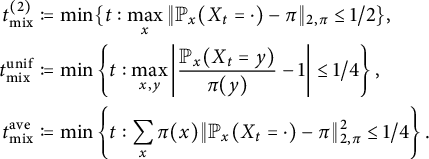
Here and below,
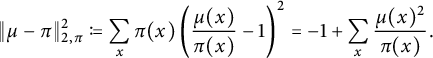
The constants $\frac 12$
and
$\frac 12$
and $\frac 14$
do not play an important role and were chosen for convenience. We remark that in the reversible setting the
$\frac 14$
do not play an important role and were chosen for convenience. We remark that in the reversible setting the $L^2$
and the
$L^2$
and the $L^\infty $
mixing times satisfy
$L^\infty $
mixing times satisfy $t_{\mathrm {mix}}^{\mathrm {unif}}=2t_{\mathrm {mix}}^{(2)}$
, while even without reversibility
$t_{\mathrm {mix}}^{\mathrm {unif}}=2t_{\mathrm {mix}}^{(2)}$
, while even without reversibility $t_{\mathrm {mix}}^{\mathrm {unif}}\le 2t_{\mathrm {mix}}^{(2)}$
. See [Reference Goel, Montenegro and Tetali20, Equation (2.2)] and [Reference Montenegro and Tetali38, Equation (8.5)] for a proof in continuous time. The proof in discrete time is similar.
$t_{\mathrm {mix}}^{\mathrm {unif}}\le 2t_{\mathrm {mix}}^{(2)}$
. See [Reference Goel, Montenegro and Tetali20, Equation (2.2)] and [Reference Montenegro and Tetali38, Equation (8.5)] for a proof in continuous time. The proof in discrete time is similar.
In the remainder of this section, we show the following.
Theorem 2.5 The average $L_2$
mixing time is robust for reversible Markov chains in continuous time.
$L_2$
mixing time is robust for reversible Markov chains in continuous time.
An immediate corollary is that the (usual, not averaged) $L_2$
mixing time is robust in the transitive setup, under perturbations that preserve transitivity (in the discrete time case assuming the holding probabilities are bounded away from 0). By the remark above, the same holds for the uniform mixing time. Theorem 2.5 is not needed for the proofs of our main results. We added it for the sake of completeness. The proof is similar to the one in [Reference Pittet and Saloff-Coste42].
$L_2$
mixing time is robust in the transitive setup, under perturbations that preserve transitivity (in the discrete time case assuming the holding probabilities are bounded away from 0). By the remark above, the same holds for the uniform mixing time. Theorem 2.5 is not needed for the proofs of our main results. We added it for the sake of completeness. The proof is similar to the one in [Reference Pittet and Saloff-Coste42].
Proof Let $\mathcal L$
be the Markov generator, and let
$\mathcal L$
be the Markov generator, and let $0 =\lambda _1 < \lambda _2 \le \cdots \le \lambda _n$
be the eigenvalues of
$0 =\lambda _1 < \lambda _2 \le \cdots \le \lambda _n$
be the eigenvalues of $-\mathcal L$
. Denote
$-\mathcal L$
. Denote $P_t=e^{t\mathcal L}$
. Then,
$P_t=e^{t\mathcal L}$
. Then,
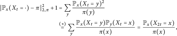 $$ \begin{align} \|{\mathbb P}_x(X_t=\cdot )-\pi \|_{2,\pi}^2+1 &=\sum_{y}\frac{{\mathbb P}_x(X_{t}=y)^{2}}{ \pi(y)}\nonumber\\ &\stackrel{(*)}{=}\sum_{y}\frac{{\mathbb P}_x(X_{t}=y){\mathbb P}_y(X_{t}=x)}{ \pi(x)} =\frac{{\mathbb P}_x(X_{2t}=x)}{\pi(x)}, \end{align} $$
where in $(*)$
we used reversibility.
$(*)$
we used reversibility.
Hence,
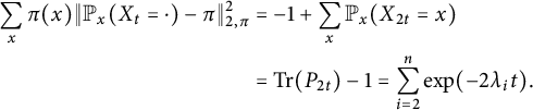 $$ \begin{align} \sum_x \pi(x)\|{\mathbb P}_x(X_t=\cdot )-\pi \|_{2,\pi}^2 &=-1+\sum_{x}{\mathbb P}_x(X_{2t}=x) \nonumber\\ &=\mathrm{Tr}(P_{2t})-1=\sum_{i=2}^n \exp(-2 \lambda_i t). \end{align} $$
Recalling the definition of the average $L_2$
mixing time, we get
$L_2$
mixing time, we get
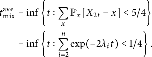 $$ \begin{align} t_{\mathrm{mix}}^{\mathrm{ave}} &= \inf \left\{t: \sum_{x}{\mathbb P}_x[X_{2t}=x] \le 5/4 \right\} \nonumber\\ &= \inf \left\{t: \sum_{i=2}^n \exp(-2\lambda_it) \le 1/4\right\}. \end{align} $$
Using (2.1) concludes the proof.
Remark 2.6 The same calculations can be done in discrete time, leading to analogs of (2.3) and (2.4): $ \sum _x \pi (x)\|{\mathbb P}_x(X_t=\cdot )-\pi \|_{2,\pi }^2 =\sum _{i=2}^n \beta _i^{2t}$
and so
$ \sum _x \pi (x)\|{\mathbb P}_x(X_t=\cdot )-\pi \|_{2,\pi }^2 =\sum _{i=2}^n \beta _i^{2t}$
and so
 $$\begin{align*}t_{\mathrm{mix}}^{\mathrm{ave}} = \inf \left\{t \in \mathbb{N} : \sum_{i=2}^n \beta_i^{2t} \le 1/4\right\}, \end{align*}$$
where $1=\beta _1>\beta _2 \ge \cdots \ge \beta _n>-1$
are the eigenvalues of the transition matrix P (assuming P is irreducible and aperiodic). This would allow to conclude a similar result in discrete time if it weren’t for values of
$1=\beta _1>\beta _2 \ge \cdots \ge \beta _n>-1$
are the eigenvalues of the transition matrix P (assuming P is irreducible and aperiodic). This would allow to conclude a similar result in discrete time if it weren’t for values of $\beta _i$
close to either 0 or
$\beta _i$
close to either 0 or $-1$
. Both problems can be resolved by adding laziness, but in the interest of brevity, we skip the details.
$-1$
. Both problems can be resolved by adding laziness, but in the interest of brevity, we skip the details.
2.3 Geometric notions
Recall from Section 1.5, the definition of $(a,b)$
-quasi-isometry for metric spaces, and that when we say that graphs are
$(a,b)$
-quasi-isometry for metric spaces, and that when we say that graphs are $(a,b)$
-quasi-isometric, we are treating them as metric spaces with the graph distance as the metric.
$(a,b)$
-quasi-isometric, we are treating them as metric spaces with the graph distance as the metric.
Definition 2.7 Consider a reversible Markov chain on a finite state space $\Omega $
with transition matrix P (in continuous time, with generator
$\Omega $
with transition matrix P (in continuous time, with generator $\mathcal L$
) and stationary distribution
$\mathcal L$
) and stationary distribution $\pi $
. We define the Cheeger constant of the chain as
$\pi $
. We define the Cheeger constant of the chain as
We will also need a version for a subset of the graph (this is the discrete analog of Dirichlet boundary conditions).
Definition 2.8 Let $\Omega $
, P,
$\Omega $
, P, $\mathcal L$
and
$\mathcal L$
and $\pi $
be as above. Let
$\pi $
be as above. Let $A \varsubsetneq \Omega $
. We define
$A \varsubsetneq \Omega $
. We define
![]() .
.
Further, we define $\lambda (A)$
to be the smallest eigenvalue of the substochastic matrix obtained by restricting
$\lambda (A)$
to be the smallest eigenvalue of the substochastic matrix obtained by restricting $I-P$
(resp.
$I-P$
(resp. $-\mathcal L$
) to A.
$-\mathcal L$
) to A.
The following discrete version of Cheeger’s inequality under Dirichlet boundary conditions is well known (see, e.g., [Reference Goel, Montenegro and Tetali20, (1.4) and Lemma 2.4]. For every irreducible discrete- or continuous-time reversible chain, and every set A with $\pi (A) \le 1/2,$
we have that
$\pi (A) \le 1/2,$
we have that
 $$ \begin{align} \Phi^2(A)/4 \le \lambda(A) \le \Phi(A), \qquad \frac{\Phi^2(A)}{4\max_{a \in A}|\mathcal L(a,a)| } \le \lambda(A) \le \Phi(A) \end{align} $$
in discrete and continuous time, respectively.
Lemma 2.9 Let G be a finite graph, v a vertex of G and $A_1,\dotsc ,A_k$
the components of
$A_1,\dotsc ,A_k$
the components of $G\setminus \{v\}$
, i.e., of G after removal of the vertex v and all adjoining edges. Let
$G\setminus \{v\}$
, i.e., of G after removal of the vertex v and all adjoining edges. Let $w_i\in A_i$
be vertices. Then the probability that random walk starting from v hits
$w_i\in A_i$
be vertices. Then the probability that random walk starting from v hits $\{w_1,\dotsc ,w_k\}$
at
$\{w_1,\dotsc ,w_k\}$
at $w_i$
is proportional to the effective conductance from v to
$w_i$
is proportional to the effective conductance from v to $w_i$
.
$w_i$
.
For a gentle introduction to electrical networks, see [Reference Doyle and Snell18].
Proof Denote by $T_{w_i}$
the hitting time of
$T_{w_i}$
the hitting time of $w_i$
and by
$w_i$
and by $T_W$
the hitting time of the set
$T_W$
the hitting time of the set $\{w_1,\dotsc ,w_k\}$
. If the walker returns to v before
$\{w_1,\dotsc ,w_k\}$
. If the walker returns to v before $T_W,$
the process begins afresh, so it is enough to consider only the last excursion from v. In other words, the probabilities are proportional to the conditioned probabilities
$T_W,$
the process begins afresh, so it is enough to consider only the last excursion from v. In other words, the probabilities are proportional to the conditioned probabilities $\mathbb {P}_v(T_{w_i}=T_W \,|\,T_W<T_v)$
(we define
$\mathbb {P}_v(T_{w_i}=T_W \,|\,T_W<T_v)$
(we define $T_v$
to be the return time to v). Since each
$T_v$
to be the return time to v). Since each $w_i$
is in a different component of
$w_i$
is in a different component of $G\setminus \{v\}$
, these conditional probabilities are proportional to
$G\setminus \{v\}$
, these conditional probabilities are proportional to $\mathbb {P}_v(T_{w_i}<T_v)$
. These are proportional to the effective conductance (see [Reference Lyons and Peres35, Exercise 2.47]).
$\mathbb {P}_v(T_{w_i}<T_v)$
. These are proportional to the effective conductance (see [Reference Lyons and Peres35, Exercise 2.47]).
Let
![]() be some graph. Let
be some graph. Let $G_{2}=(V_{2},E_{2})$
be a graph obtained from
$G_{2}=(V_{2},E_{2})$
be a graph obtained from $G_{1}$
by “stretching” some of the edges of
$G_{1}$
by “stretching” some of the edges of $G_{1}$
by a factor of at most K (we say that
$G_{1}$
by a factor of at most K (we say that $G_{2}$
is a K-stretch of
$G_{2}$
is a K-stretch of $G_{1}$
). That is, for some
$G_{1}$
). That is, for some $E \subset E_{1}$
, we replace each edge
$E \subset E_{1}$
, we replace each edge $uv\in E $
by a path of length at most K (whose endpoints are still denoted by u and v). Note that
$uv\in E $
by a path of length at most K (whose endpoints are still denoted by u and v). Note that $V_{1} \subset V_{2}$
. The identity map is a
$V_{1} \subset V_{2}$
. The identity map is a $(K,0)$
-quasi-isometry of
$(K,0)$
-quasi-isometry of $G_1$
and
$G_1$
and $G_2$
.
$G_2$
.
Lemma 2.10 There exists a constant $c_d> 0$
(depending only on d) such that if H is a simple graph of maximal degree d and G is a K-stretch of H, then
$c_d> 0$
(depending only on d) such that if H is a simple graph of maximal degree d and G is a K-stretch of H, then
 $$ \begin{align} \Phi(G) \ge c_d \Phi(H)/K, \end{align} $$
where $\Phi (G)$
and
$\Phi (G)$
and $\Phi (H)$
are the Cheeger constants of G and H, respectively.
$\Phi (H)$
are the Cheeger constants of G and H, respectively.
This is well known and easy to see (see, e.g., [Reference Hermon24, Proposition 2.3] for a proof). We finish this section with a simple lemma on stretched trees.
Lemma 2.11 Let T be a finite binary tree of height $\ell $
, let
$\ell $
, let $f:\{1,\dotsc ,\ell \}\to \mathbb {N}$
be non-increasing, and let G be the graph one gets by stretching each edge between levels
$f:\{1,\dotsc ,\ell \}\to \mathbb {N}$
be non-increasing, and let G be the graph one gets by stretching each edge between levels $h-1$
and h of T to a path of length
$h-1$
and h of T to a path of length $f(h)$
. Then, for every v in level h of T, we have
$f(h)$
. Then, for every v in level h of T, we have
 $$\begin{align*}{\mathbb P}_G(\textrm{random walk starting from v hits the root before hitting level }\ell)\le 2^{-h}. \end{align*}$$
Proof The symmetry of the problem allows us to identify all the vertices in each level of T (before stretching). Consider the probability that random walk starting from v hits level $\ell $
before hitting the root. After the identification, we have the following.
$\ell $
before hitting the root. After the identification, we have the following.
-
• Level $\ell $
is just one vertex (which we also denote by
$\ell $
).
$\ell $
is just one vertex (which we also denote by
$\ell $
). -
• Removing the vertex corresponding to level h (which we also denote by v) disconnects the root from
$\ell $
.


Hence, Lemma 2.9 may be used. Suppressing the dependence on $\ell $
, denote the resistances from the root and from v to
$\ell $
, denote the resistances from the root and from v to $\ell $
by
$\ell $
by $R_1$
and
$R_1$
and $R_2$
, respectively. Then the probability to hit the root before hitting
$R_2$
, respectively. Then the probability to hit the root before hitting $\ell $
is
$\ell $
is $R_2/R_1$
. These resistances can be computed directly using parallel-series laws. Indeed, the resistance of
$R_2/R_1$
. These resistances can be computed directly using parallel-series laws. Indeed, the resistance of $f(i)$
edges in a series is
$f(i)$
edges in a series is $f(i)$
and the resistance of
$f(i)$
and the resistance of $2^i$
parallel connections of this kind between i and
$2^i$
parallel connections of this kind between i and $i+1$
is
$i+1$
is $2^{-i}f(i)$
. All in all, we get
$2^{-i}f(i)$
. All in all, we get
 $$\begin{align*}R_1 =\sum_{i=1}^{\ell}\frac{f(i)}{2^i}\ge \sum_{i=1}^\ell \frac{f(i+h)}{2^{i}} \ge \sum_{i=1}^{\ell-h}\frac{f(i+h)}{2^i}=2^{h}R_2, \end{align*}$$
where the first inequality follows because f is non-increasing. The assertion of lemma follows.
2.4 A tail estimate for hitting times
Recall that the hitting time of a set D is defined as
![]() . Denote
. Denote $\pi $
conditioned on A by
$\pi $
conditioned on A by $\pi _A$
, i.e.,
$\pi _A$
, i.e.,
![]() . Using the spectral decomposition of
. Using the spectral decomposition of $P_A$
(the restriction of the transition matrix P to the set A) with respect to the inner product
$P_A$
(the restriction of the transition matrix P to the set A) with respect to the inner product
![]() , we get (see, e.g., [Reference Aldous and Fill3, Chapter 3] or [Reference Basu, Hermon and Peres6, Lemma 3.8]),
, we get (see, e.g., [Reference Aldous and Fill3, Chapter 3] or [Reference Basu, Hermon and Peres6, Lemma 3.8]),
 $$ \begin{align} \min_{x,y \in A} \frac{\pi(x)}{|A|\pi(y)} \sum_{a \in A} {\mathbb P}_{a }[T_{ A^{c}}> t]\le {\mathbb P}_{\pi_A}[T_{ A^{c}} > t] \le e^{- \lambda(A)t} \end{align} $$
in discrete or continuous time.
3 Proof of Theorems 1.1 and 1.2
Throughout this section, we consider the interchange process on a graph G in continuous time in which all edges ring at rate 1 (Theorems 1.1 and 1.2 are formulated in discrete time, but translating the mixing time from continuous time to discrete time is simple and we explain this for Theorem 1.1 at the end of its proof, the explanation there holds for Theorem 1.2 equally). Since the claims of both theorems are asymptotic, we may and will assume that n is sufficiently large.
Let us start the proof by recalling elements of the construction already discussed in the proof sketch in Section 1.3 and in other places in the introduction. We need to find a set of transpositions $S_n\subset \mathfrak {S}_n$
such that
$S_n\subset \mathfrak {S}_n$
such that $t_{\mathrm {mix}}(\operatorname {\mathrm {Cay}}(\mathfrak {S}_n,S_n))$
is small compared to either
$t_{\mathrm {mix}}(\operatorname {\mathrm {Cay}}(\mathfrak {S}_n,S_n))$
is small compared to either $t_{\mathrm {mix}}(\operatorname {\mathrm {Cay}}(\mathfrak {S}_n,S_n'))$
for a second set of transpositions
$t_{\mathrm {mix}}(\operatorname {\mathrm {Cay}}(\mathfrak {S}_n,S_n'))$
for a second set of transpositions $S_n'$
such that
$S_n'$
such that $S_n\subseteq S_n'\subseteq S_n^3$
(in Theorem 1.1) or to
$S_n\subseteq S_n'\subseteq S_n^3$
(in Theorem 1.1) or to $t_{\mathrm {mix}}(\operatorname {\mathrm {Cay}}(\mathfrak {S}_n,S_n,W_n))$
for some weights
$t_{\mathrm {mix}}(\operatorname {\mathrm {Cay}}(\mathfrak {S}_n,S_n,W_n))$
for some weights $W_n$
(in Theorem 1.2). We describe our set of transpositions using a graph G on n vertices, whose edges are the transpositions. The construction has two parameters,
$W_n$
(in Theorem 1.2). We describe our set of transpositions using a graph G on n vertices, whose edges are the transpositions. The construction has two parameters, $u\in \mathbb {N}$
and
$u\in \mathbb {N}$
and $\epsilon \in (0,\frac 12)$
(both will be chosen later). We designate u parts of G and call them
$\epsilon \in (0,\frac 12)$
(both will be chosen later). We designate u parts of G and call them $H_1,\dotsc ,H_u$
(we will use
$H_1,\dotsc ,H_u$
(we will use $H_i$
to denote both a subset of
$H_i$
to denote both a subset of $[n]$
and the induced subgraph, and we will now describe them as graphs, thus describing also a part of G). The
$[n]$
and the induced subgraph, and we will now describe them as graphs, thus describing also a part of G). The $H_i$
are constructed inductively as follows. The induction base,
$H_i$
are constructed inductively as follows. The induction base, $H_1$
is a binary tree of depth u whose edges have been replaced by paths of length
$H_1$
is a binary tree of depth u whose edges have been replaced by paths of length $2^{u}$
. To define
$2^{u}$
. To define $H_{i+1}$
given
$H_{i+1}$
given $H_{i}$
we label, in each vertex of each of the trees used to construct
$H_{i}$
we label, in each vertex of each of the trees used to construct $H_{i}$
one child as “left” and the other as “right.” We denote, for each leaf v of
$H_{i}$
one child as “left” and the other as “right.” We denote, for each leaf v of $H_{i}$
, the number of left children on the path from the root to v by
$H_{i}$
, the number of left children on the path from the root to v by $g(v)$
. Recall the definition of the bad leaves
$g(v)$
. Recall the definition of the bad leaves $B_{i}$
,
$B_{i}$
,
from (1.4). We define $H_{i+1}$
as a forest of
$H_{i+1}$
as a forest of $|B_{i}|$
binary trees of depth
$|B_{i}|$
binary trees of depth $s_{i+1}$
, with each edge replaced by a path of length
$s_{i+1}$
, with each edge replaced by a path of length $\ell _{i+1}$
, with
$\ell _{i+1}$
, with
and each tree rooted at a point of $B_{i}$
(so
$B_{i}$
(so $H_{i+1}\cap H_{i}=B_{i}$
as sets). This terminates the description of the
$H_{i+1}\cap H_{i}=B_{i}$
as sets). This terminates the description of the $H_i$
. All this, we remind, was already discussed in Section 1.3 with some additional explanations and motivation (and a figure depicting the gadget
$H_i$
. All this, we remind, was already discussed in Section 1.3 with some additional explanations and motivation (and a figure depicting the gadget $\bigcup H_i$
on page 30).
$\bigcup H_i$
on page 30).
We now claim that, uniformly in ${\varepsilon }$
,
${\varepsilon }$
,
 $$\begin{align*}2^{4^{u-1}u}\le \bigg|\bigcup_{i=1}^u H_i\bigg|\le 2^{4^{u}u}. \end{align*}$$
Indeed, the first inequality is clear because $H_u$
has at least one root (since
$H_u$
has at least one root (since $\epsilon <\frac 12$
) and the second inequality comes from
$\epsilon <\frac 12$
) and the second inequality comes from
 $$\begin{align*}|H_i|\le \ell_i2^{s_i+1}|B_{i-1}| \le 2^{u+2-i+4^{i-1}u}\prod_{j=1}^{i-1}2^{4^{j-1}u} \le 2^{u+2-i+4^{i-1}u(1+1/3)}\le 2^{3\cdot 4^{i-1}u}, \end{align*}$$
which can be summed readily to give
 $$ \begin{align} \sum_{j=1}^i|H_j|\le 2^{4^iu}, \end{align} $$
and in particular, the case $i=u$
is what we need. Hence, we may choose some
$i=u$
is what we need. Hence, we may choose some $u=u_n$
such that
$u=u_n$
such that $u4^u\asymp \log n$
(in particular,
$u4^u\asymp \log n$
(in particular, $u\asymp \log \log n$
) such that
$u\asymp \log \log n$
) such that
 $$ \begin{align} \sum_{i=1}^u|H_i|\le n^{1/4}, \end{align} $$
regardless of $\epsilon $
(we need here
$\epsilon $
(we need here $n\ge 65,\!536$
to have
$n\ge 65,\!536$
to have $2^{4^uu}\le n^{1/4}$
for
$2^{4^uu}\le n^{1/4}$
for $u=1$
). Fix such a u for the rest of the proof.
$u=1$
). Fix such a u for the rest of the proof.
The subgraph $\bigcup H_i$
is the “gadget,” and the rest of the graph G is a complete graph on a set of vertices K. The gadget connects to the complete graph via the good leaves of the
$\bigcup H_i$
is the “gadget,” and the rest of the graph G is a complete graph on a set of vertices K. The gadget connects to the complete graph via the good leaves of the $H_i$
(and all the leaves of the last one,
$H_i$
(and all the leaves of the last one, $H_u$
) so we define K to also include those vertices. Thus, we define
$H_u$
) so we define K to also include those vertices. Thus, we define

Let the edges of G be all the edges of all the $H_i$
union with a complete graph on K, i.e.,
$H_i$
union with a complete graph on K, i.e.,
This finishes the construction of G (except for the choice of $\epsilon $
), and hence of
$\epsilon $
), and hence of $S_n$
. We delay the definitions of
$S_n$
. We delay the definitions of $S_n'$
and
$S_n'$
and $W_n$
to Section 3.3.
$W_n$
to Section 3.3.
Below, when we want to emphasize the dependence on u and $\varepsilon ,$
we will write
$\varepsilon ,$
we will write $G_n(u,\varepsilon )$
for G and
$G_n(u,\varepsilon )$
for G and $S_n(u,\varepsilon )$
for
$S_n(u,\varepsilon )$
for $S_n$
. We will also denote
$S_n$
. We will also denote
![]() and
and
![]() (recall that
(recall that $u_n$
is the value we fixed above such that
$u_n$
is the value we fixed above such that $u_n4^{u_n}\asymp \log n$
).
$u_n4^{u_n}\asymp \log n$
).
3.1 An upper bound for the time to exit the gadget
Throughout the proofs, we will pick the parameter $\varepsilon $
so that
$\varepsilon $
so that $\epsilon>u^{-1/3}$
.
$\epsilon>u^{-1/3}$
.
Lemma 3.1 The expected exit time from $H_i$
, starting from a worst initial state in
$H_i$
, starting from a worst initial state in $H_i$
(i.e., the one maximizing this expectation), denoted by
$H_i$
(i.e., the one maximizing this expectation), denoted by $L_i$
, satisfies (uniformly in i)
$L_i$
, satisfies (uniformly in i)
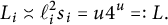 $$ \begin{align} L_i \asymp\ell_i^2s_i = u4^u=:L. \end{align} $$
As this lemma is standard, we only sketch its proof.
Proof sketch
Examine the random walk X on $H_i$
, and let
$H_i$
, and let $\sigma _0,\sigma _1,\dotsc $
be the times when it reaches a vertex of degree 3 (we require also
$\sigma _0,\sigma _1,\dotsc $
be the times when it reaches a vertex of degree 3 (we require also $X_{\sigma _{i+1}}\ne X_{\sigma _i}$
). Between
$X_{\sigma _{i+1}}\ne X_{\sigma _i}$
). Between $\sigma _i$
and
$\sigma _i$
and $\sigma _{i+1}$
, the walk is in a part of the graph which is simply three paths of length
$\sigma _{i+1}$
, the walk is in a part of the graph which is simply three paths of length $\ell _i$
. By symmetry, it reaches each of the 3 ends of these lines with equal probability. Hence,
$\ell _i$
. By symmetry, it reaches each of the 3 ends of these lines with equal probability. Hence, $X_{\sigma _i}$
is identical to a random walk on a binary tree of depth
$X_{\sigma _i}$
is identical to a random walk on a binary tree of depth $s_i$
. The distance of random walk on a binary tree from the root has the same distribution as a random walk on
$s_i$
. The distance of random walk on a binary tree from the root has the same distribution as a random walk on $\mathbb {N}$
with a drift toward infinity, and hence, a simple calculation shows that the expected exit time is
$\mathbb {N}$
with a drift toward infinity, and hence, a simple calculation shows that the expected exit time is $Cs_i$
. To get back to random walk on
$Cs_i$
. To get back to random walk on $H_i$
, we note that, even if we condition on
$H_i$
, we note that, even if we condition on $X_{\sigma _0},X_{\sigma _1},\dotsc $
, then the local symmetry says that the times
$X_{\sigma _0},X_{\sigma _1},\dotsc $
, then the local symmetry says that the times $\sigma _{i+1}-\sigma _i$
are independent of
$\sigma _{i+1}-\sigma _i$
are independent of $X_{\sigma _i}$
and of one another. For each i, we have
$X_{\sigma _i}$
and of one another. For each i, we have $\mathbb E(\sigma _{i+1}-\sigma _i)\asymp \ell _i^2$
, because this is the same as the exit time from the interval
$\mathbb E(\sigma _{i+1}-\sigma _i)\asymp \ell _i^2$
, because this is the same as the exit time from the interval $\{0,\dotsc ,\ell _i\}$
, where the walk exits 0 at rate 3 (and the other vertices at rate 2), again by the symmetry.
$\{0,\dotsc ,\ell _i\}$
, where the walk exits 0 at rate 3 (and the other vertices at rate 2), again by the symmetry.
Below, we employ the notation $L=u4^u$
from the above lemma. Let
$L=u4^u$
from the above lemma. Let $ T_{K}:=\inf \{t:X_t \in K \}$
be the hitting time of the complete graph K. Recall that we have fixed a choice of
$ T_{K}:=\inf \{t:X_t \in K \}$
be the hitting time of the complete graph K. Recall that we have fixed a choice of $u=u_n$
satisfying that
$u=u_n$
satisfying that $u4^u\asymp \log n$
.
$u4^u\asymp \log n$
.
Proposition 3.2 There exist some constants C and $c'$
such that, for every
$c'$
such that, for every $\varepsilon $
and
$\varepsilon $
and $n,$
we have that the graph
$n,$
we have that the graph $G_n(\varepsilon )$
satisfies for all
$G_n(\varepsilon )$
satisfies for all $i\in [u]$
that
$i\in [u]$
that
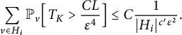 $$ \begin{align} \sum_{v \in H_{i} }{\mathbb P}_v\Big[T_{K}> \frac{CL}{\epsilon^4} \Big] \le C \frac{1}{|H_{i}|^{c'\epsilon^2}}.\end{align} $$
Consequently, if E is the event that, for all $i \in [u]$
, all particles whose initial location is in
$i \in [u]$
, all particles whose initial location is in $ H_i$
hit the complete graph K before time
$ H_i$
hit the complete graph K before time $CL/\epsilon ^4$
, then
$CL/\epsilon ^4$
, then $\lim _{n\to \infty } {\mathbb P}(E)=1$
, uniformly in
$\lim _{n\to \infty } {\mathbb P}(E)=1$
, uniformly in $\epsilon $
.
$\epsilon $
.
We recall our standing assumptions that n is sufficiently large and that $\epsilon>u_n^{-1/3}$
(in particular, “uniformly in
$\epsilon>u_n^{-1/3}$
(in particular, “uniformly in $\epsilon $
” above means “uniformly in
$\epsilon $
” above means “uniformly in $\epsilon \in (u^{1/3},\frac 12)$
”). Let us remark that the
$\epsilon \in (u^{1/3},\frac 12)$
”). Let us remark that the $\epsilon ^4$
term is not optimal, but this is not a priority for us.
$\epsilon ^4$
term is not optimal, but this is not a priority for us.
Proof of Proposition 3.2
The assertion of the last sentence of the proposition follows from (3.5) by a union bound over the particles (recall that in the interchange process, each particle is performing a random walk). We also need here our assumption that $\epsilon> u^{-1/3}$
, as it gives
$\epsilon> u^{-1/3}$
, as it gives $\sum _{i=1}^u 1/|H_i|^{c\epsilon ^2}=o(1) $
, since
$\sum _{i=1}^u 1/|H_i|^{c\epsilon ^2}=o(1) $
, since $|H_i| \ge 2^{s_i} = 2^{4^{i-1}u}$
.
$|H_i| \ge 2^{s_i} = 2^{4^{i-1}u}$
.
Thus, we need to verify (3.5). Let $m=m(\epsilon )\ge 1$
be some integer parameter to be fixed later. Let
$m=m(\epsilon )\ge 1$
be some integer parameter to be fixed later. Let
where $T_{[n]\setminus W_i}$
is the hitting time of
$T_{[n]\setminus W_i}$
is the hitting time of $[n]\setminus W_i$
(or the exit time of
$[n]\setminus W_i$
(or the exit time of $W_i$
, if you prefer). The proof of Proposition 3.2 is concluded by combining the following two lemmas. Indeed, let m be the minimal value which satisfies the requirement of Lemma 3.4, so
$W_i$
, if you prefer). The proof of Proposition 3.2 is concluded by combining the following two lemmas. Indeed, let m be the minimal value which satisfies the requirement of Lemma 3.4, so $4^m\asymp \epsilon ^{-2}$
. We use the same value of m in Lemma 3.3 and get that for
$4^m\asymp \epsilon ^{-2}$
. We use the same value of m in Lemma 3.3 and get that for $t>CL/\epsilon ^4$
we have (3.6). Combining this with (3.7) gives the proposition.
$t>CL/\epsilon ^4$
we have (3.6). Combining this with (3.7) gives the proposition.
Lemma 3.3 For all $i\in [u]$
and all
$i\in [u]$
and all $t\ge C_116^mL$
for some
$t\ge C_116^mL$
for some $C_1$
sufficiently large,
$C_1$
sufficiently large,
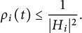 $$ \begin{align} \rho_i(t)\le \frac{1}{|H_i|^2}. \end{align} $$
(As usual, $C_1$
is an absolute constant. In particular, it depends on neither i nor t.)
$C_1$
is an absolute constant. In particular, it depends on neither i nor t.)
Lemma 3.4 There exist absolute constants $C,c>0$
such that for all
$C,c>0$
such that for all $\varepsilon \in (0,1/2)$
, if
$\varepsilon \in (0,1/2)$
, if $4^m\epsilon ^2 \ge C$
, then, for all
$4^m\epsilon ^2 \ge C$
, then, for all $n \ge N_0$
, the graph
$n \ge N_0$
, the graph $G(n,u,\varepsilon )$
satisfies for every
$G(n,u,\varepsilon )$
satisfies for every $i\in [u]$
that
$i\in [u]$
that
 $$ \begin{align} \sum_{v \in H_{i} }{\mathbb P}_v[T_{[n]\setminus W_i} <T_{K}] \le \frac{C}{|H_{i}|^{c\epsilon^2}}. \end{align} $$
Proof of Lemma 3.3
Let $\mathcal M$
be the restriction of the Markov generator
$\mathcal M$
be the restriction of the Markov generator $\mathcal L$
to
$\mathcal L$
to $W_i \setminus K $
(i.e., this is the generator of the chain killed upon exiting
$W_i \setminus K $
(i.e., this is the generator of the chain killed upon exiting $W_i \setminus K $
). Let
$W_i \setminus K $
). Let $\lambda $
be the smallest eigenvalue of
$\lambda $
be the smallest eigenvalue of $-\mathcal M$
. It will be convenient to extend the definition
$-\mathcal M$
. It will be convenient to extend the definition $\ell _{i} =2^{u+1-i}$
also to negative i. We now claim that
$\ell _{i} =2^{u+1-i}$
also to negative i. We now claim that
 $$ \begin{align} \lambda \gtrsim \ell_{i-m}^{-2}. \end{align} $$
To see this, let W be an arbitrary connected component of $W_i$
. We first apply Lemma 2.10 to W. Since it is a piece of an infinite binary tree with edges stretched to various extents, but not more than
$W_i$
. We first apply Lemma 2.10 to W. Since it is a piece of an infinite binary tree with edges stretched to various extents, but not more than $\ell _{i-m}$
, and since the infinite tree has positive Cheeger constant, we get that the Cheeger constant of W is at least
$\ell _{i-m}$
, and since the infinite tree has positive Cheeger constant, we get that the Cheeger constant of W is at least $\ell _{i-m}^{-1}$
. Applying Cheeger’s inequality (2.5) to
$\ell _{i-m}^{-1}$
. Applying Cheeger’s inequality (2.5) to $W\setminus K$
embedded in an infinite, stretched tree shows (3.8).
$W\setminus K$
embedded in an infinite, stretched tree shows (3.8).
Using this, we get that
 $$ \begin{align} \begin{aligned} \rho_i(t) & \stackrel{\textrm{(2.7)}}{\le} |W_i| \exp(- \lambda t ) \stackrel{\text{(3.8,3.2)}}{\le} 2^{4^{i+m}u} \exp(-c\ell_{i-m}^{-2}t ) \\ &\,\stackrel{(*)}{\le} 2^{4^{i+m}u} \exp(-c 4^{i-u-m-1}\cdot C_116^m\cdot u4^u ) \stackrel{\textrm{(3.2)}}{\le} \frac{1}{|H_{i}|^{2}}, \end{aligned} \end{align} $$
where the inequality marked $(*)$
follows from the definitions of
$(*)$
follows from the definitions of $\ell _i$
and L (recall that
$\ell _i$
and L (recall that $L=u4^u$
) and from the bound on t in the statement of the lemma. In the last inequality, we also use that
$L=u4^u$
) and from the bound on t in the statement of the lemma. In the last inequality, we also use that $C_1$
is sufficiently large.
$C_1$
is sufficiently large.
Proof of Lemma 3.4
We divide the event $T_{[n]\setminus W_i}<T_{K}$
into two cases: that the random walk hits
$T_{[n]\setminus W_i}<T_{K}$
into two cases: that the random walk hits $H_{i+m+1}$
before hitting K, and that it hits
$H_{i+m+1}$
before hitting K, and that it hits $H_{i-m-1}$
before hitting K. Denote these two events by
$H_{i-m-1}$
before hitting K. Denote these two events by ${\mathcal U}$
and
${\mathcal U}$
and ${\mathcal D}$
, respectively (notice that if
${\mathcal D}$
, respectively (notice that if $i\ge u-m$
then
$i\ge u-m$
then ${\mathcal U}$
is empty and if
${\mathcal U}$
is empty and if $i\le m+1$
then
$i\le m+1$
then ${\mathcal D}$
is empty). The letters
${\mathcal D}$
is empty). The letters ${\mathcal U}$
and
${\mathcal U}$
and ${\mathcal D}$
stand for “up” and “down,” with the orientation being as in Figure 1 (page 30).
${\mathcal D}$
stand for “up” and “down,” with the orientation being as in Figure 1 (page 30).
We first handle ${\mathcal U}$
. For
${\mathcal U}$
. For ${\mathcal U}$
to happen there must be some time
${\mathcal U}$
to happen there must be some time $\sigma <T_K$
such that
$\sigma <T_K$
such that $X_{\sigma }\in B_{i+m-1} \subset H_{i+m}$
and, further, the walker is contained in
$X_{\sigma }\in B_{i+m-1} \subset H_{i+m}$
and, further, the walker is contained in $H_{i+m}$
between time
$H_{i+m}$
between time $\sigma $
and the first hitting time to the set of leaves of
$\sigma $
and the first hitting time to the set of leaves of $H_{i+m}$
which (on the event
$H_{i+m}$
which (on the event ${\mathcal U}$
) occurs at
${\mathcal U}$
) occurs at $B_{i+m}$
. Assume such a
$B_{i+m}$
. Assume such a $\sigma $
exists and examine the walker between
$\sigma $
exists and examine the walker between $\sigma $
and
$\sigma $
and $T_{B_{i+m}}$
. The walker is not simple (because being after
$T_{B_{i+m}}$
. The walker is not simple (because being after $\sigma $
conditions it to not return to the roots of
$\sigma $
conditions it to not return to the roots of $H_{i+m}$
) but this is not important for us. The symmetry of the tree implies that at the first time after
$H_{i+m}$
) but this is not important for us. The symmetry of the tree implies that at the first time after $\sigma $
that the walker visits a leaf of
$\sigma $
that the walker visits a leaf of $H_{i+m}$
, the difference between the number of left and right turns along the path the walker takes is distributed like a sum of i.i.d.
$H_{i+m}$
, the difference between the number of left and right turns along the path the walker takes is distributed like a sum of i.i.d. $\pm 1$
variables (giving equal probability to each value). In particular, the probability that the target leaf is in
$\pm 1$
variables (giving equal probability to each value). In particular, the probability that the target leaf is in $B_{i+m}$
is
$B_{i+m}$
is
 $$\begin{align*}{\mathbb P}\Big(\textrm{Bin}(s_{i+m},\tfrac 12)>\big(\tfrac 12+\epsilon\big)s_{i+m}\Big)\le \exp(-c\epsilon^2s_{i+m}). \end{align*}$$
Our assumption that a time $\sigma $
exists only reduces the probability further so we get, for every
$\sigma $
exists only reduces the probability further so we get, for every $v\in H_i$
, that
$v\in H_i$
, that ${\mathbb P}_v({\mathcal U})\le \exp (-c\epsilon ^2s_{i+m})$
. Summing over v gives
${\mathbb P}_v({\mathcal U})\le \exp (-c\epsilon ^2s_{i+m})$
. Summing over v gives
 $$\begin{align*}\sum_{v\in H_i}{\mathbb P}_v({\mathcal U})\le |H_i|\exp(-c\epsilon^2s_{i+m}) \stackrel{\textrm{(3.2)}}{\le} 2^{4^iu}\exp(-c\epsilon^24^{i+m}u), \end{align*}$$
and we see that if m satisfies $4^m\ge 2/c\epsilon ^2$
then this sum is smaller than, say,
$4^m\ge 2/c\epsilon ^2$
then this sum is smaller than, say, $1/|H_i|^2$
. Require m to satisfy that, but do not fix its value yet (there will be a similar requirement below).
$1/|H_i|^2$
. Require m to satisfy that, but do not fix its value yet (there will be a similar requirement below).
We move to the estimate of ${\mathcal D}$
. We use Lemma 2.11 and get that for any v in level h of
${\mathcal D}$
. We use Lemma 2.11 and get that for any v in level h of $H_i$
(we are counting levels before stretching here) or in the path between level h and
$H_i$
(we are counting levels before stretching here) or in the path between level h and $h+1$
, we have
$h+1$
, we have
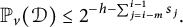 $$\begin{align*}{\mathbb P}_v({\mathcal D})\le 2^{-h-\sum_{j=i-m}^{i-1}s_{j}}. \end{align*}$$
(Note that Lemma 2.11 measures a larger event. Indeed, ${\mathcal D}$
is the event to hit the root of our tree before hitting level
${\mathcal D}$
is the event to hit the root of our tree before hitting level $i+m$
or K, so it is smaller than the event to hit the root before
$i+m$
or K, so it is smaller than the event to hit the root before $i+m$
, which is what is measured by Lemma 2.11.) The number of vertices at level h, or in a path between level h and
$i+m$
, which is what is measured by Lemma 2.11.) The number of vertices at level h, or in a path between level h and $h+1$
, is
$h+1$
, is $|B_{i-1}|\cdot 2^h\cdot \ell _i$
, so we get
$|B_{i-1}|\cdot 2^h\cdot \ell _i$
, so we get
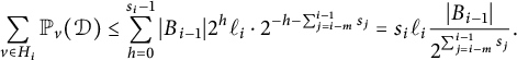 $$ \begin{align} \sum_{v\in H_i}{\mathbb P}_v({\mathcal D})\le\sum_{h=0}^{s_i-1}|B_{i-1}|2^{h}\ell_i\cdot 2^{-h-\sum_{j=i-m}^{i-1}s_{j}}=s_i\ell_i\frac{|B_{i-1}|}{ 2^{\sum_{j=i-m}^{i-1}s_{j}}}. \end{align} $$
Denote $p_j:={\mathbb P}\big (\textrm {Bin}(s_{j},\tfrac 12)>(\tfrac 12+\epsilon )s_{j}\big )$
. Then
$p_j:={\mathbb P}\big (\textrm {Bin}(s_{j},\tfrac 12)>(\tfrac 12+\epsilon )s_{j}\big )$
. Then $|B_{j}| \le |B_{j-1}|2^{s_{j}}p_{j}$
and further
$|B_{j}| \le |B_{j-1}|2^{s_{j}}p_{j}$
and further $p_j \le \exp \left (-c\epsilon ^2 s_{j}\right ) $
. Iterating this gives
$p_j \le \exp \left (-c\epsilon ^2 s_{j}\right ) $
. Iterating this gives
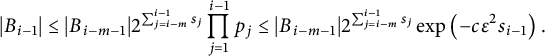 $$\begin{align*}|B_{i-1}| \le |B_{i-m-1}|2^{\sum_{j=i-m}^{i-1}s_{j}}\prod_{j=1}^{i-1}p_j \le |B_{i-m-1}|2^{\sum_{j=i-m}^{i-1}s_{j}}\exp \left(-c\epsilon^2 s_{i-1}\right). \end{align*}$$
Substituting this in (3.10) gives
We see that taking m so that $4^{m}\epsilon ^2 $
is sufficiently large makes the term
$4^{m}\epsilon ^2 $
is sufficiently large makes the term $2^{4^{i-m-1}u}=2^{s_{i-1}4^{-m+1}}$
negligible compared to the exponential (recall that
$2^{4^{i-m-1}u}=2^{s_{i-1}4^{-m+1}}$
negligible compared to the exponential (recall that $s_i=4^{i-1}u$
). This is the last requirement from m and we may fix its value. Further, our standing assumption that
$s_i=4^{i-1}u$
). This is the last requirement from m and we may fix its value. Further, our standing assumption that $\epsilon>u^{-1/3}$
means that the
$\epsilon>u^{-1/3}$
means that the $s_i\ell _i$
terms are also negligible with respect to
$s_i\ell _i$
terms are also negligible with respect to $\exp (-c\epsilon ^2s_{i-1})$
. Hence
$\exp (-c\epsilon ^2s_{i-1})$
. Hence
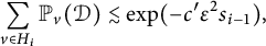 $$\begin{align*}\sum_{v\in H_i}{\mathbb P}_v({\mathcal D})\lesssim \exp(-c'\epsilon^2s_{i-1}), \end{align*}$$
as needed. The lemma is thus proved, and so is Proposition 3.2.
Having established in Proposition 3.2 that the walker hits K, we now show that it remains there for a considerable amount of time.
Lemma 3.5 Let
![]() for some
for some $C_1$
sufficiently large. For every
$C_1$
sufficiently large. For every $x\in [n]$
, let
$x\in [n]$
, let $N(x)$
be the amount of time a walker starting from x spends in K up to time t. Then
$N(x)$
be the amount of time a walker starting from x spends in K up to time t. Then
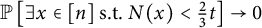 $$\begin{align*}{\mathbb P}\left[\exists x\in[n]\textrm{ s.t. }N(x)<\tfrac 23 t\right]\to 0 \end{align*}$$
as $n\to \infty $
, uniformly in
$n\to \infty $
, uniformly in $\epsilon>u^{-1/3}$
(but not necessarily in
$\epsilon>u^{-1/3}$
(but not necessarily in $C_1$
).
$C_1$
).
Proof Let $q=C_2L/\epsilon ^4$
, where
$q=C_2L/\epsilon ^4$
, where $C_2$
is the constant from Proposition 3.2, denoted there by C. Apply Proposition 3.2 after some arbitrary time s. We get that during the interval
$C_2$
is the constant from Proposition 3.2, denoted there by C. Apply Proposition 3.2 after some arbitrary time s. We get that during the interval $[s,s+q]$
, the probability that all particles in
$[s,s+q]$
, the probability that all particles in $[n]\setminus K$
hit K is at least
$[n]\setminus K$
hit K is at least
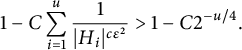 $$\begin{align*}1-C\sum_{i=1}^u \frac{1}{|H_i|^{c\epsilon^2}}>1-C2^{-u/4}. \end{align*}$$
Hence, for any fixed value of $C_1$
, we can apply this for
$C_1$
, we can apply this for $s=0,q,2q,\dotsc ,q(\lfloor t/q\rfloor -1)$
(just a constant number of times, in fact
$s=0,q,2q,\dotsc ,q(\lfloor t/q\rfloor -1)$
(just a constant number of times, in fact $\lfloor C_1/C_2\rfloor $
) and get that with probability going to 1, all events happen simultaneously. In other words, no particle spent more than
$\lfloor C_1/C_2\rfloor $
) and get that with probability going to 1, all events happen simultaneously. In other words, no particle spent more than $2q$
consecutive time units in any visit of
$2q$
consecutive time units in any visit of $[n]\setminus K$
.
$[n]\setminus K$
.
Let us now bound the number of possible visits. We will show that a.a.s. as $n\to \infty $
no particle makes more than one visit to
$n\to \infty $
no particle makes more than one visit to $[n] \setminus K$
by time t after reaching K for the first time. For this purpose, denote
$[n] \setminus K$
by time t after reaching K for the first time. For this purpose, denote $\partial K$
to be all points of K with a neighbor in
$\partial K$
to be all points of K with a neighbor in $[n]\setminus K$
(namely, leaves of
$[n]\setminus K$
(namely, leaves of $H_i$
which are not in
$H_i$
which are not in $B_i$
for
$B_i$
for $i<u$
and all leaves of
$i<u$
and all leaves of $H_u$
).
$H_u$
).
Suppose a particle is at time $0$
at some
$0$
at some $x\in K$
. Let us first bound the number of jumps it does up to time t. Since the degrees of our graph are all bounded by
$x\in K$
. Let us first bound the number of jumps it does up to time t. Since the degrees of our graph are all bounded by $|K|$
, this number is stochastically dominated by an appropriate Poisson variable, and in particular, the probability that the particle performed more than
$|K|$
, this number is stochastically dominated by an appropriate Poisson variable, and in particular, the probability that the particle performed more than $2t|K|$
jumps is
$2t|K|$
jumps is $o(1/n)$
. Adding the restriction that the jump would be to a vertex of K only reduces the number further, so we get the same bound for the number of jumps to vertices of K.
$o(1/n)$
. Adding the restriction that the jump would be to a vertex of K only reduces the number further, so we get the same bound for the number of jumps to vertices of K.
Among the first $2t|K|$
jumps to vertices of K, the number of jumps to
$2t|K|$
jumps to vertices of K, the number of jumps to $\partial K$
is stochastically dominated by
$\partial K$
is stochastically dominated by $\mathrm {Bin}(2t|K|,\frac {|\partial K|}{|K|-1}) $
. Hence, the probability that more than
$\mathrm {Bin}(2t|K|,\frac {|\partial K|}{|K|-1}) $
. Hence, the probability that more than $4t|\partial K|$
of them are to
$4t|\partial K|$
of them are to $\partial K$
is
$\partial K$
is $o(1/n)$
(where we used that
$o(1/n)$
(where we used that $|\partial K| \gtrsim n^c $
, which follows from our choice of u).
$|\partial K| \gtrsim n^c $
, which follows from our choice of u).
Examine now the first $4t|\partial K|+2$
visits to
$4t|\partial K|+2$
visits to $\partial K$
(not necessarily up to time t, all of them). The probability that at least two of the following jumps were away from K is at most
$\partial K$
(not necessarily up to time t, all of them). The probability that at least two of the following jumps were away from K is at most $(4t|\partial K|+2)^{2}/|K|^{2}=o(1/n)$
, where we used the fact that by (3.3)
$(4t|\partial K|+2)^{2}/|K|^{2}=o(1/n)$
, where we used the fact that by (3.3) $|\partial K|\le n^{1/4}$
and
$|\partial K|\le n^{1/4}$
and $|K| \ge n-n^{1/4}$
, as well as
$|K| \ge n-n^{1/4}$
, as well as $t \lesssim \log ^2 n$
(recall that
$t \lesssim \log ^2 n$
(recall that $L\asymp \log n$
and
$L\asymp \log n$
and $\epsilon>u^{-1/3}\asymp (\log \log n)^{-1/3}$
). In the case that indeed no more than 1 of these jumps went to
$\epsilon>u^{-1/3}\asymp (\log \log n)^{-1/3}$
). In the case that indeed no more than 1 of these jumps went to $[n]\setminus K$
, we get that the first
$[n]\setminus K$
, we get that the first $4t|\partial K|+2$
visits to
$4t|\partial K|+2$
visits to $\partial K$
include all the visits to
$\partial K$
include all the visits to $\partial K$
up to time t: no more than
$\partial K$
up to time t: no more than $4t|\partial K|$
visits from K and no more than 2 visits from
$4t|\partial K|$
visits from K and no more than 2 visits from $[n]\setminus K$
(the first hitting of K and the first return to K).
$[n]\setminus K$
(the first hitting of K and the first return to K).
Combining everything together, we see that after first reaching K (which a.a.s. all particles do by time q) a.a.s. all particles leave K at most once by time t and during such excursion they each spend at most $2q$
time units away from K. Taking
$2q$
time units away from K. Taking $C_1$
to be large enough in terms of
$C_1$
to be large enough in terms of $C_2$
concludes the proof.
$C_2$
concludes the proof.
3.2 The coupling
Denote the transposition $(x,y)$
by
$(x,y)$
by $\tau _{xy}$
. Consider two initial configurations
$\tau _{xy}$
. Consider two initial configurations $\sigma $
and
$\sigma $
and $\sigma '$
of the interchange process. We now define a coupling
$\sigma '$
of the interchange process. We now define a coupling $((\sigma _t)_{t \ge 0}, (\sigma ^{\prime }_t)_{t \ge 0})$
of the interchange processes starting from these initial states. We make the edges ring at rate 2, but when an edge rings, it is ignored with probability
$((\sigma _t)_{t \ge 0}, (\sigma ^{\prime }_t)_{t \ge 0})$
of the interchange processes starting from these initial states. We make the edges ring at rate 2, but when an edge rings, it is ignored with probability $1/2$
. We use the same clocks for both systems. If, at time
$1/2$
. We use the same clocks for both systems. If, at time $t,$
an edge
$t,$
an edge $e=xy$
rings and
$e=xy$
rings and $\sigma _{t-}(x)=\sigma ^{\prime }_{t-}(y)$
(where
$\sigma _{t-}(x)=\sigma ^{\prime }_{t-}(y)$
(where
![]() , as usual) or
, as usual) or $\sigma _{t-}(y)=\sigma ^{\prime }_{t-}(x),$
then with probability 1/2, we set
$\sigma _{t-}(y)=\sigma ^{\prime }_{t-}(x),$
then with probability 1/2, we set $\sigma _t=\sigma _{t-} \circ \tau _{e}$
and
$\sigma _t=\sigma _{t-} \circ \tau _{e}$
and $\sigma ^{\prime }_{t}=\sigma ^{\prime }_{t-}$
; and with probability
$\sigma ^{\prime }_{t}=\sigma ^{\prime }_{t-}$
; and with probability $1/2,$
we set
$1/2,$
we set $\sigma _t=\sigma _{t-} $
and
$\sigma _t=\sigma _{t-} $
and $\sigma ^{\prime }_{t}=\sigma ^{\prime }_{t-} \circ \tau _e$
(either way, the number of disagreements decreases). If
$\sigma ^{\prime }_{t}=\sigma ^{\prime }_{t-} \circ \tau _e$
(either way, the number of disagreements decreases). If $\sigma _{t-}(x) \neq \sigma ^{\prime }_{t-}(y)$
and
$\sigma _{t-}(x) \neq \sigma ^{\prime }_{t-}(y)$
and $\sigma _{t-}(y)\neq \sigma ^{\prime }_{t-}(x),$
then with probability 1/2, we set
$\sigma _{t-}(y)\neq \sigma ^{\prime }_{t-}(x),$
then with probability 1/2, we set $\sigma _t=\sigma _{t-} \circ \tau _{e}$
and
$\sigma _t=\sigma _{t-} \circ \tau _{e}$
and $\sigma _t'=\sigma _{t-} ' \circ \tau _{e}$
; and with probability 1/2, we set
$\sigma _t'=\sigma _{t-} ' \circ \tau _{e}$
; and with probability 1/2, we set $\sigma _t=\sigma _{t-} $
and
$\sigma _t=\sigma _{t-} $
and $\sigma _t'=\sigma _{t-} '$
.
$\sigma _t'=\sigma _{t-} '$
.
We see that for all i once the particle labeled i is coupled in the two systems, it remains coupled. That is, if $\sigma _{t}^{-1}(i)=(\sigma ^{\prime }_{t})^{-1}(i),$
then, for
$\sigma _{t}^{-1}(i)=(\sigma ^{\prime }_{t})^{-1}(i),$
then, for $t'>t,$
we also have
$t'>t,$
we also have $\sigma _{t'}^{-1}(i)=(\sigma ^{\prime }_{t'})^{-1}(i)$
. Whenever the position of particle i is adjacent in one system is adjacent to the current position of particle i in the other system (i.e.,
$\sigma _{t'}^{-1}(i)=(\sigma ^{\prime }_{t'})^{-1}(i)$
. Whenever the position of particle i is adjacent in one system is adjacent to the current position of particle i in the other system (i.e., $\sigma _{t}^{-1}(i)(\sigma ^{\prime }_{t})^{-1}(i) \in E_n$
), the infinitesimal rate in which they are coupled is
$\sigma _{t}^{-1}(i)(\sigma ^{\prime }_{t})^{-1}(i) \in E_n$
), the infinitesimal rate in which they are coupled is $2$
.
$2$
.
Lemma 3.6 There exists a C such that
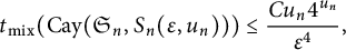 $$\begin{align*}t_{\mathrm{mix}}(\operatorname{\mathrm{Cay}}(\mathfrak{S}_n,S_n(\epsilon,u_n)))\le \frac{Cu_n4^{u_n}}{\epsilon^4}, \end{align*}$$
under our usual assumption that $\epsilon>u_n^{-1/3}$
.
$\epsilon>u_n^{-1/3}$
.
Proof Lemma 3.5 shows that a.a.s. indeed all particles in one system spend at least $\frac {2}{3}$
of the time in K by time
$\frac {2}{3}$
of the time in K by time $C_1L/\epsilon ^4$
for any
$C_1L/\epsilon ^4$
for any $C_1$
sufficiently large. By a union bound, this applies to both systems in the above coupling. On this event (occurring for both systems), for each
$C_1$
sufficiently large. By a union bound, this applies to both systems in the above coupling. On this event (occurring for both systems), for each $i,$
the particle labeled i has to spend at least
$i,$
the particle labeled i has to spend at least $1/3$
of the time by time
$1/3$
of the time by time $C_1L/\epsilon ^4$
in K simultaneously in both systems. Since the particle gets coupled with rate 2 during these times, a standard argument shows that the conditional probability of particle i not getting coupled is at most
$C_1L/\epsilon ^4$
in K simultaneously in both systems. Since the particle gets coupled with rate 2 during these times, a standard argument shows that the conditional probability of particle i not getting coupled is at most
 $$ \begin{align} \exp(-cC_1 L/\epsilon^4)\le\exp(-cC_1L) \stackrel{(*)}{\le}n^{-cC_1}, \end{align} $$
where the inequality marked by $(*)$
follows since
$(*)$
follows since $L=u4^u\asymp \log n$
(see just above (3.3)). If
$L=u4^u\asymp \log n$
(see just above (3.3)). If $C_1$
is sufficiently large, this will be
$C_1$
is sufficiently large, this will be $\ll 1/n$
and we may apply a union bound and get that a.a.s. all particles are coupled by time
$\ll 1/n$
and we may apply a union bound and get that a.a.s. all particles are coupled by time $C_1L/\epsilon ^4$
. As the initial states
$C_1L/\epsilon ^4$
. As the initial states $\sigma $
and
$\sigma $
and $\sigma '$
are arbitrary, this implies that the mixing time is at most
$\sigma '$
are arbitrary, this implies that the mixing time is at most $C_1L/\epsilon ^4$
(see, e.g., [Reference Levin, Peres, Wilmer, Propp and Wilson33, Theorem 5.4]).
$C_1L/\epsilon ^4$
(see, e.g., [Reference Levin, Peres, Wilmer, Propp and Wilson33, Theorem 5.4]).
3.3 The perturbation
In this section, we analyze the perturbed versions of $S_n$
, lower bound their mixing time, and thus conclude the proofs of Theorems 1.1 and 1.2. The following convention will be useful here and in other places in the paper. Thus, we make special note of it
$S_n$
, lower bound their mixing time, and thus conclude the proofs of Theorems 1.1 and 1.2. The following convention will be useful here and in other places in the paper. Thus, we make special note of it
Definition 3.7 We call an edge of $H_i$
that belongs to a path that is a stretching of a left edge (of
$H_i$
that belongs to a path that is a stretching of a left edge (of $H_i'$
) a “left edge.” Similarly for right edges.
$H_i'$
) a “left edge.” Similarly for right edges.
Do not be confused with the definition of g. It is still the case that g counts left edges before stretching, not all left edges of $H_i$
.
$H_i$
.
Proof of Theorem 1.2
Recall that we are given a function $1\ll f(n)\le \log \log \log n$
and we need to construct generators
$1\ll f(n)\le \log \log \log n$
and we need to construct generators $S_n$
and weights
$S_n$
and weights $W_n=(w_n(s))_{s\in S}$
satisfying
$W_n=(w_n(s))_{s\in S}$
satisfying $1\le w_n(s)\le 1+(f(n!)/\log \log n)^{1/4}$
such that
$1\le w_n(s)\le 1+(f(n!)/\log \log n)^{1/4}$
such that
 $$\begin{align*}t_{\mathrm{mix}}(\operatorname{\mathrm{Cay}}(\mathfrak{S}_{n},S_{n},W_n)) \gtrsim t_{\mathrm{mix}}(\operatorname{\mathrm{Cay}}(\mathfrak{S}_{n},S_{n}))f(n!). \end{align*}$$
Define
![]() , where
, where $c_1$
is a universal positive constant that will be fixed soon (but let us already require
$c_1$
is a universal positive constant that will be fixed soon (but let us already require $c_1<\frac 14$
). The requirement
$c_1<\frac 14$
). The requirement $\epsilon>u^{-1/3}$
will be satisfied for n sufficiently large. We use the set
$\epsilon>u^{-1/3}$
will be satisfied for n sufficiently large. We use the set $S_n(u,\epsilon )$
defined above with
$S_n(u,\epsilon )$
defined above with $u=u_n$
and this
$u=u_n$
and this $\epsilon $
(we remind that
$\epsilon $
(we remind that $u_n\asymp \log \log n$
).
$u_n\asymp \log \log n$
).
Denote, for any $\delta>0$
,
$\delta>0$
, $W(\delta ,n)=(w(s))_{s\in S_n}$
with
$W(\delta ,n)=(w(s))_{s\in S_n}$
with

(“otherwise” referring to both right edges and to edges of K). We will take $\delta =\epsilon /c_1$
in what follows. The notation
$\delta =\epsilon /c_1$
in what follows. The notation $W(\delta ,n)$
will be reused below in the proof of Theorem 1.1, but there we will take
$W(\delta ,n)$
will be reused below in the proof of Theorem 1.1, but there we will take $\delta =3$
, so let us proceed under the assumption
$\delta =3$
, so let us proceed under the assumption $\delta \le 3$
, which holds under the definitions of
$\delta \le 3$
, which holds under the definitions of $\delta $
and
$\delta $
and $\epsilon $
above too.
$\epsilon $
above too.
Recall the notation $g(v)$
for the number of left children in a path from the root to v (before stretching). Examine first an infinite binary tree where each left child has weight
$g(v)$
for the number of left children in a path from the root to v (before stretching). Examine first an infinite binary tree where each left child has weight $1+\delta $
for some
$1+\delta $
for some $\delta>0$
, and each right child has weight 1 (denote this object by
$\delta>0$
, and each right child has weight 1 (denote this object by ${\mathcal T}_\delta $
). Let
${\mathcal T}_\delta $
). Let $Y_k$
be the last vertex in the
$Y_k$
be the last vertex in the $k{\textrm {th}}$
level visited by random walk on it. By [Reference Hermon and Peres26, Fact 4.1(2a)] (proved in the appendix of [Reference Hermon and Peres26]),
$k{\textrm {th}}$
level visited by random walk on it. By [Reference Hermon and Peres26, Fact 4.1(2a)] (proved in the appendix of [Reference Hermon and Peres26]), $g(Y_k)$
has the same distribution as the sum of k independent
$g(Y_k)$
has the same distribution as the sum of k independent $\{0,1\}$
-variables taking the value 1 with probability
$\{0,1\}$
-variables taking the value 1 with probability
 $$\begin{align*}\frac{\sqrt{1+\delta}}{1+\sqrt{1+\delta}}=\frac{1}{2}+\delta/8+O(\delta^2). \end{align*}$$
This fact holds also for random walk on ${\mathcal T}_\delta $
started from either child of the root and conditioned not to return to the root. The proof in [Reference Hermon and Peres26] applies to this case verbatim. Now, if
${\mathcal T}_\delta $
started from either child of the root and conditioned not to return to the root. The proof in [Reference Hermon and Peres26] applies to this case verbatim. Now, if $c_1$
is sufficiently small, then
$c_1$
is sufficiently small, then
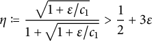
(recall that $\delta =\epsilon /c_1$
is bounded above by
$\delta =\epsilon /c_1$
is bounded above by $3$
). Fix
$3$
). Fix $c_1$
to satisfy this property.
$c_1$
to satisfy this property.
Still on the infinite tree ${\mathcal T}_{\delta }$
, denote by
${\mathcal T}_{\delta }$
, denote by $Y_k^*$
, the vertex where the walker is at on the first time, it hits level k, in other words, the hitting point. It is straightforward to see that
$Y_k^*$
, the vertex where the walker is at on the first time, it hits level k, in other words, the hitting point. It is straightforward to see that ${\mathbb P}(|g(Y_k^*)-g(Y_k)|>\lambda )\le 2e^{-c\lambda }$
for every
${\mathbb P}(|g(Y_k^*)-g(Y_k)|>\lambda )\le 2e^{-c\lambda }$
for every $\lambda $
, where the (nonnegative) constant c is independent of
$\lambda $
, where the (nonnegative) constant c is independent of $\epsilon $
.
$\epsilon $
.
Information on $Y_k^*$
can already be translated to our graphs
$Y_k^*$
can already be translated to our graphs $H_i$
, because random walk on
$H_i$
, because random walk on $H_i$
, when considered only at times when it reaches a vertex before stretching, is identical to random walk on a piece of
$H_i$
, when considered only at times when it reaches a vertex before stretching, is identical to random walk on a piece of ${\mathcal T}_{\epsilon /c_1}$
(say, by Lemma 2.9). We get that a random walk starting from a root of
${\mathcal T}_{\epsilon /c_1}$
(say, by Lemma 2.9). We get that a random walk starting from a root of $H_i$
and conditioned not to go to
$H_i$
and conditioned not to go to $H_{i-1}$
before leaving
$H_{i-1}$
before leaving $H_i$
(for
$H_i$
(for $i=1$
, an unconditioned walker) has, when it exits
$i=1$
, an unconditioned walker) has, when it exits $H_i$
that g is distributed like
$H_i$
that g is distributed like $\textrm {Bin}(s_i,\eta )$
plus a quantity with a uniform exponential tail (uniform in both i and the value attained by the
$\textrm {Bin}(s_i,\eta )$
plus a quantity with a uniform exponential tail (uniform in both i and the value attained by the $\textrm {Bin}(s_i,\eta )$
random variable).
$\textrm {Bin}(s_i,\eta )$
random variable).
A similar argument shows that, now on our graphs $H_i$
, if
$H_i$
, if $Z_i$
is the first vertex, the walker is in among the roots of
$Z_i$
is the first vertex, the walker is in among the roots of $H_{i+1}$
(which of course is also a leaf of
$H_{i+1}$
(which of course is also a leaf of $H_i$
) and
$H_i$
) and $Z_i^*$
is the last vertex, the walker is in
$Z_i^*$
is the last vertex, the walker is in $H_i$
(say, before hitting the leaves of
$H_i$
(say, before hitting the leaves of $H_{i+1}$
or K for the first time), then
$H_{i+1}$
or K for the first time), then $|g(Z_i)-g(Z_i^*)|$
is bounded with an exponential tail (uniformly in i).
$|g(Z_i)-g(Z_i^*)|$
is bounded with an exponential tail (uniformly in i).
We may now finish the proof of the theorem. Indeed, let X be the particle that was at time 0 at the root of $H_1$
. Let T be the time X hits the leaves of
$H_1$
. Let T be the time X hits the leaves of $H_1$
. We see that, if
$H_1$
. We see that, if $\lambda>0$
is some sufficiently small constant, then
$\lambda>0$
is some sufficiently small constant, then
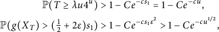 $$ \begin{align*} {\mathbb P}(T\ge \lambda u4^u)&>1-Ce^{-cs_1}=1-Ce^{-cu},\\ {\mathbb P}(g(X_T)>(\tfrac12 +2\epsilon)s_1)&>1-Ce^{-cs_1\epsilon^2}>1-Ce^{-cu^{1/2}}, \end{align*} $$
where the last inequality is due to $\epsilon \gtrsim (\log \log n)^{-1/4}$
. In particular, with the same probability
$\epsilon \gtrsim (\log \log n)^{-1/4}$
. In particular, with the same probability $X_T$
is in
$X_T$
is in $B_1$
. The same X still has that
$B_1$
. The same X still has that $g>(\frac 12+\epsilon )s_1$
when leaving
$g>(\frac 12+\epsilon )s_1$
when leaving $H_1$
(again with probability
$H_1$
(again with probability $>1-Ce^{-cs_1\epsilon ^2}$
), and then hits the leaves of
$>1-Ce^{-cs_1\epsilon ^2}$
), and then hits the leaves of $H_2$
after another at least
$H_2$
after another at least $\lambda u4^u$
time units, and hits
$\lambda u4^u$
time units, and hits $B_2$
, and so on. We get that, at time
$B_2$
, and so on. We get that, at time $\lambda u^24^u$
, this particle is still inside the gadget, with probability at least
$\lambda u^24^u$
, this particle is still inside the gadget, with probability at least $1-Cue^{-cu^{1/2}}$
. This of course means the walk on
$1-Cue^{-cu^{1/2}}$
. This of course means the walk on $\mathfrak {S}_n$
is not yet mixed. Hence
$\mathfrak {S}_n$
is not yet mixed. Hence
 $$\begin{align*}t_{\mathrm{mix}}(\operatorname{\mathrm{Cay}}(\mathfrak{S}_n,S_n,W_n))\gtrsim u^24^u. \end{align*}$$
With Lemma 3.6, we get that
 $$\begin{align*}t_{\mathrm{mix}}(\operatorname{\mathrm{Cay}}(\mathfrak{S}_n,S_n,W_n))\gtrsim u^24^u\gtrsim t_{\mathrm{mix}}(\operatorname{\mathrm{Cay}}(\mathfrak{S}_n,S_n)) \cdot u\epsilon^4\asymp t_{\mathrm{mix}}(\operatorname{\mathrm{Cay}}(\mathfrak{S}_n,S_n))f(n!) \end{align*}$$
as claimed (in the last “ $\asymp $
” we used
$\asymp $
” we used $u \asymp \log \log n$
). This concludes the proof.
$u \asymp \log \log n$
). This concludes the proof.
Proof of Theorem 1.1
Recall from the proof sketch Section 1.3 that $S_n'$
is created by adding to each path of
$S_n'$
is created by adding to each path of $S_n$
that came from stretching a left edge, edges between even vertices (initially at distance two from one another). The parallel–serial laws show that the resistance of a path of length
$S_n$
that came from stretching a left edge, edges between even vertices (initially at distance two from one another). The parallel–serial laws show that the resistance of a path of length $2N$
to which such edges have been added is
$2N$
to which such edges have been added is $\frac 23 N$
. Examining a walker only at times where it is in vertices that were not added in the stretching process, we see that its walk is exactly identical to a walk on
$\frac 23 N$
. Examining a walker only at times where it is in vertices that were not added in the stretching process, we see that its walk is exactly identical to a walk on $\operatorname {\mathrm {Cay}}(\mathfrak {S}_n,S_n,W(3,n))$
, where
$\operatorname {\mathrm {Cay}}(\mathfrak {S}_n,S_n,W(3,n))$
, where $W(3,n)$
is from the previous proof. Hence choosing
$W(3,n)$
is from the previous proof. Hence choosing $\epsilon =3c_1$
, we get, as in the previous proof,
$\epsilon =3c_1$
, we get, as in the previous proof, $t_{\mathrm {mix}}(\operatorname {\mathrm {Cay}}(\mathfrak {S}_n,S_n'))\gtrsim u^24^u$
.
$t_{\mathrm {mix}}(\operatorname {\mathrm {Cay}}(\mathfrak {S}_n,S_n'))\gtrsim u^24^u$
.
This almost finishes the proof of Theorem 1.1. The only remaining issue to address is that Theorem 1.1 is formulated in discrete time, while we worked all along in continuous time. This is not a problem. Indeed, if P is a transition matrix and I is the identity matrix, then the total variation mixing time $t_{\mathrm {mix}}^{\delta \, \mathrm {lazy}}$
of the
$t_{\mathrm {mix}}^{\delta \, \mathrm {lazy}}$
of the $\delta $
-lazy chain with transition matrix
$\delta $
-lazy chain with transition matrix $\delta I+(1-\delta ) P$
and that of the continuous-time chain with generator
$\delta I+(1-\delta ) P$
and that of the continuous-time chain with generator $\mathcal L=P-I$
, denoted by
$\mathcal L=P-I$
, denoted by $t_{\mathrm {mix}}^{\mathrm {ct}} $
, satisfy
$t_{\mathrm {mix}}^{\mathrm {ct}} $
, satisfy
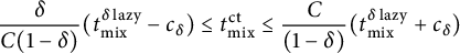 $$ \begin{align} \frac{\delta}{C(1-\delta) } (t_{\mathrm{mix}}^{\delta \, \mathrm{lazy}}-c_{\delta})\le t_{\mathrm{mix}}^{\mathrm{ct}} \le \frac{C}{(1-\delta) }(t_{\mathrm{mix}}^{\delta \, \mathrm{lazy}}+c_{\delta}) \end{align} $$
for an absolute constant $C>0$
and a constant
$C>0$
and a constant $c_{\delta }>0$
, independent of the Markov chain. The case
$c_{\delta }>0$
, independent of the Markov chain. The case $\delta =1/2$
follows directly from [Reference Levin, Peres, Wilmer, Propp and Wilson33, Theorem 20.3] and the argument extends to all
$\delta =1/2$
follows directly from [Reference Levin, Peres, Wilmer, Propp and Wilson33, Theorem 20.3] and the argument extends to all $\delta \in (0,1) $
. For much finer relations between the two mixing times in the reversible setup, see [Reference Basu, Hermon and Peres6, Reference Chen and Saloff-Coste13, Reference Hermon and Peres27].
$\delta \in (0,1) $
. For much finer relations between the two mixing times in the reversible setup, see [Reference Basu, Hermon and Peres6, Reference Chen and Saloff-Coste13, Reference Hermon and Peres27].
In our case, we estimated the continuous time mixing time with the rates equal to 1, while the generator $\mathcal L$
has rates
$\mathcal L$
has rates $1/|S_n|$
or
$1/|S_n|$
or $1/|S_n'|$
, as the case may be. Multiplying all the rates by a constant changes the mixing time by the same constant, so we get
$1/|S_n'|$
, as the case may be. Multiplying all the rates by a constant changes the mixing time by the same constant, so we get
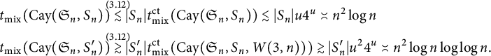
The theorem is thus proved.
4 Proof of Theorem 1.3
Recall that we wish to construct a sequence of graphs $G_n$
with bounded degrees and weights with
$G_n$
with bounded degrees and weights with $1\le w_n(e)\le 1+o(1)$
such that the mixing time of
$1\le w_n(e)\le 1+o(1)$
such that the mixing time of $G_n$
is significantly smaller than the mixing time of the weighted version.
$G_n$
is significantly smaller than the mixing time of the weighted version.
As a building block in our construction, we will need the auxiliary graph described in the following lemma, whose proof is deferred to Section 4.4.
Lemma 4.1 There exists an absolute constant $\mu>0 $
such that, for every
$\mu>0 $
such that, for every $m,$
there exists a graph H of maximal degree
$m,$
there exists a graph H of maximal degree $6$
with
$6$
with $|H| \asymp 2^{10m}$
containing two disjoint sets of vertices B and W of sizes
$|H| \asymp 2^{10m}$
containing two disjoint sets of vertices B and W of sizes $|B|=2^m$
and
$|B|=2^m$
and $|W|= 2^{10m}$
such that lazy SRW on H satisfies that
$|W|= 2^{10m}$
such that lazy SRW on H satisfies that
 $$ \begin{align} {\mathbb P}_b[T_{B \setminus \{b\}} < T_{W} ]&\lesssim 2^{-4m} \qquad\ \ \ \, \forall b\in B, \end{align} $$
 $$ \begin{align} \mathbb E_h[T_{B \setminus \{h\}}] &\asymp |H|/2^m \qquad \forall h\in H, \end{align} $$
 $$ \begin{align} {\mathbb P}_h[T_{B \setminus \{h\}}>|H|/2^m] &\gtrsim 1 \qquad \forall h\in H, \end{align} $$
 $$ \begin{align} {\mathbb P}_b[T_W<T_b\,|\,T_W<T_{B\setminus \{b\}}] &\ge\mu \qquad \forall b\in B. \end{align} $$
Moreover, the last probability is the same for all $b \in B$
. Lastly, for all
$b \in B$
. Lastly, for all $w\in W$
starting from w the hitting distribution of B uniform.
$w\in W$
starting from w the hitting distribution of B uniform.
As usual, $T_W$
,
$T_W$
, $T_B$
, etc. are the hitting times of B, W, etc.
$T_B$
, etc. are the hitting times of B, W, etc.
4.1 The construction
Let $G=G_n((\log \log n)^{-1/8}),$
i.e., the graph from the construction of Theorem 1.2 with the parameter
$G=G_n((\log \log n)^{-1/8}),$
i.e., the graph from the construction of Theorem 1.2 with the parameter $\epsilon $
from the construction taken to be
$\epsilon $
from the construction taken to be $(\log \log n)^{-1/8}$
(G is the graph on which the interchange process is performed, so
$(\log \log n)^{-1/8}$
(G is the graph on which the interchange process is performed, so $E(G)$
is a set of transpositions of
$E(G)$
is a set of transpositions of $\mathfrak {S}_n$
). Let m satisfy that
$\mathfrak {S}_n$
). Let m satisfy that $2^{m-1}< |E(G)|\le 2^{m}$
. Let H be the graph from Lemma 4.1 with this m (so
$2^{m-1}< |E(G)|\le 2^{m}$
. Let H be the graph from Lemma 4.1 with this m (so $|H| \asymp 2^{10m} \asymp n^{20}$
). Let
$|H| \asymp 2^{10m} \asymp n^{20}$
). Let $A\subseteq B$
(B from the statement of Lemma 4.1) be some arbitrary set of size
$A\subseteq B$
(B from the statement of Lemma 4.1) be some arbitrary set of size $|E(G)|,$
and let
$|E(G)|,$
and let $\tau :A\to E(G)$
be some arbitrary bijection.
$\tau :A\to E(G)$
be some arbitrary bijection.
We now construct our graph, which we denote by L. We take the vertex set to be $H\times \mathfrak {S}_n$
. We define the edges implicitly by describing the transition probabilities of the random walk. Let
$H\times \mathfrak {S}_n$
. We define the edges implicitly by describing the transition probabilities of the random walk. Let $\{a,b\}\in E(H)$
. If
$\{a,b\}\in E(H)$
. If $a\not \in A,$
we set
$a\not \in A,$
we set $P\left (\left (a,\sigma \right ),\left (b,\sigma \right ) \right )=\frac {1}{\deg a}$
for all
$P\left (\left (a,\sigma \right ),\left (b,\sigma \right ) \right )=\frac {1}{\deg a}$
for all $\sigma \in \mathfrak {S}_n$
, where
$\sigma \in \mathfrak {S}_n$
, where $\deg a$
is the degree of a in H. If
$\deg a$
is the degree of a in H. If $a \in A$
and
$a \in A$
and $b \in H \setminus A, $
we set
$b \in H \setminus A, $
we set $P\left (\left (a,\sigma \right ),\left (b,\sigma \right ) \right )=\frac {1}{2\deg a}$
, while
$P\left (\left (a,\sigma \right ),\left (b,\sigma \right ) \right )=\frac {1}{2\deg a}$
, while $P\left (\left (a,\sigma \right ),\left ( a,\sigma \circ \tau _{a} \right ) \right )=\frac {1}{2}$
(recall that
$P\left (\left (a,\sigma \right ),\left ( a,\sigma \circ \tau _{a} \right ) \right )=\frac {1}{2}$
(recall that $\tau _a$
is the transposition corresponding to a). No other transitions have positive probability. Below, we consider the mixing time of the continuous time version of P or the discrete time mixing time of
$\tau _a$
is the transposition corresponding to a). No other transitions have positive probability. Below, we consider the mixing time of the continuous time version of P or the discrete time mixing time of $\frac 12 (I+P)$
. We shall denote either mixing time by
$\frac 12 (I+P)$
. We shall denote either mixing time by $t_{\mathrm {mix}}(L)$
.
$t_{\mathrm {mix}}(L)$
.
This chain $(X_t,\sigma _t)_{t \ge 0}$
can be described as follows: We have a random walk
$(X_t,\sigma _t)_{t \ge 0}$
can be described as follows: We have a random walk $(X_t)_{t \ge 0}$
on H and an “interchange process”
$(X_t)_{t \ge 0}$
on H and an “interchange process” $\sigma _t$
on G which evolves in slow motion. Whenever the walk
$\sigma _t$
on G which evolves in slow motion. Whenever the walk $X_t$
on H is at some vertex
$X_t$
on H is at some vertex $a \in A$
, it either stays put or makes a random walk step on H. If it stays put in
$a \in A$
, it either stays put or makes a random walk step on H. If it stays put in $a \in A,$
then it also makes one step of the interchange process, updating its state to
$a \in A,$
then it also makes one step of the interchange process, updating its state to $\sigma _t \circ \tau _a$
.
$\sigma _t \circ \tau _a$
.
4.2 Analysis of the example
We first define a sequence of random times. Recall the set W from the construction of H in Lemma 4.1. Let
and
. Inductively, set
Let ${\mathcal J}$
be the event that, for all
${\mathcal J}$
be the event that, for all $i \le n^4,$
the walk does not visit
$i \le n^4,$
the walk does not visit $B \setminus \{X_{T_i}\} $
between time
$B \setminus \{X_{T_i}\} $
between time $T_i$
and
$T_i$
and $S_{i+1}$
. By (4.1),
$S_{i+1}$
. By (4.1), ${\mathbb P}_{y}(\mathcal {J})> 1-O(n^{-4})$
for all
${\mathbb P}_{y}(\mathcal {J})> 1-O(n^{-4})$
for all $y\in L$
.
$y\in L$
.
Let $Z_i:=X_{T_i}$
and
$Z_i:=X_{T_i}$
and $\widehat \sigma _{i}:= \sigma _{T_i}$
(
$\widehat \sigma _{i}:= \sigma _{T_i}$
( $\sigma _{t}$
being the second coordinate of the chain
$\sigma _{t}$
being the second coordinate of the chain $(X_t,\sigma _t)$
). By Lemma 4.1, we have that
$(X_t,\sigma _t)$
). By Lemma 4.1, we have that $Z_1,\ldots ,Z_{n^4}$
are i.i.d. uniform on B. Under
$Z_1,\ldots ,Z_{n^4}$
are i.i.d. uniform on B. Under ${\mathcal J}$
, the behavior of the permutation
${\mathcal J}$
, the behavior of the permutation $\sigma $
in the time interval
$\sigma $
in the time interval $[T_i,T_{i+1})$
is quite simple: if
$[T_i,T_{i+1})$
is quite simple: if $Z_i\in B\setminus A,$
then it does not change at all in this interval, and if
$Z_i\in B\setminus A,$
then it does not change at all in this interval, and if $Z_i\in A,$
then it is composed with
$Z_i\in A,$
then it is composed with $\tau _{Z_i}$
with probability
$\tau _{Z_i}$
with probability $\frac 12$
for each time
$\frac 12$
for each time $t\in [T_i,T_{i+1})$
when
$t\in [T_i,T_{i+1})$
when $X_t=Z_i$
. This, together with (4.4) imply that, still under
$X_t=Z_i$
. This, together with (4.4) imply that, still under $\mathcal {J}$
,
$\mathcal {J}$
, $(\widehat \sigma _i)_{i=1}^{n^4}$
evolves precisely like a lazy version of the discrete-time interchange process on G. The laziness has two sources: the probability to hit
$(\widehat \sigma _i)_{i=1}^{n^4}$
evolves precisely like a lazy version of the discrete-time interchange process on G. The laziness has two sources: the probability to hit $B\setminus A$
(which gives laziness
$B\setminus A$
(which gives laziness $|B\setminus A|/|B|$
, which is bounded above by
$|B\setminus A|/|B|$
, which is bounded above by $\frac 12$
), and an additional laziness coming from the event of applying the transposition
$\frac 12$
), and an additional laziness coming from the event of applying the transposition $\tau _{Z_i}$
an even number of times between
$\tau _{Z_i}$
an even number of times between $T_i$
and
$T_i$
and $S_{i+1}$
. We use here the fact that the probability in (4.4) is the same for all
$S_{i+1}$
. We use here the fact that the probability in (4.4) is the same for all $a \in A$
. In other words, we have a coupling of
$a \in A$
. In other words, we have a coupling of $\widehat \sigma _i$
and lazy interchange on G which succeeds (i.e., the two processes are the same) with probability
$\widehat \sigma _i$
and lazy interchange on G which succeeds (i.e., the two processes are the same) with probability $1-O(n^{-4})$
.
$1-O(n^{-4})$
.
Let r be the $\frac 14$
total variation mixing time of this lazy discrete-time interchange process on G. To estimate r, note that by Lemma 3.6, the mixing time of the interchange process is at most
$\frac 14$
total variation mixing time of this lazy discrete-time interchange process on G. To estimate r, note that by Lemma 3.6, the mixing time of the interchange process is at most $Cu4^u\epsilon ^{-4}\asymp \log n(\log \log n)^{1/2}$
(recall that
$Cu4^u\epsilon ^{-4}\asymp \log n(\log \log n)^{1/2}$
(recall that $ u4^u \asymp \log n$
). Using (3.12), we may translate this to the mixing time of the lazy discrete-time interchange process and get that
$ u4^u \asymp \log n$
). Using (3.12), we may translate this to the mixing time of the lazy discrete-time interchange process and get that $r\lesssim n^2 \log n(\log \log n)^{1/2}$
(recall that
$r\lesssim n^2 \log n(\log \log n)^{1/2}$
(recall that $|E(G)| \asymp n^2$
). In particular,
$|E(G)| \asymp n^2$
). In particular, $r<n^4$
for all sufficiently large n.
$r<n^4$
for all sufficiently large n.
Thus, under ${\mathcal J}$
, we have that
${\mathcal J}$
, we have that $X_{T_{r+1}}$
has its first coordinate uniform on B and its second approximately uniform on
$X_{T_{r+1}}$
has its first coordinate uniform on B and its second approximately uniform on $\mathfrak {S}_n$
and independent of the first coordinate. Removing the requirement that we are on
$\mathfrak {S}_n$
and independent of the first coordinate. Removing the requirement that we are on $\mathcal {J}$
, the distribution of
$\mathcal {J}$
, the distribution of $X_{T_{r+1}}$
is still approximately uniform (in the TV distance) on the same set, simply because
$X_{T_{r+1}}$
is still approximately uniform (in the TV distance) on the same set, simply because ${\mathbb P}(\mathcal {J})>1-Cn^{-4}$
.
${\mathbb P}(\mathcal {J})>1-Cn^{-4}$
.
In the language of [Reference Lovász, Winkler, Aldous and Propp34], $T_{r+1}$
is an approximate forget time. As we recall below, by combining results from [Reference Aldous2] and [Reference Lovász, Winkler, Aldous and Propp34], this implies that
$T_{r+1}$
is an approximate forget time. As we recall below, by combining results from [Reference Aldous2] and [Reference Lovász, Winkler, Aldous and Propp34], this implies that
 $$ \begin{align} t_{\mathrm{mix}}(L)\lesssim \max_{y} \mathbb E_y (T_{r+1}) \stackrel{\textrm{(4.2)}}{\asymp} (r+2)\frac{|H|}{2^m}\lesssim n^{20}\log n\sqrt{\log\log n} \end{align} $$
(we have $r+2$
rather than
$r+2$
rather than $r+1$
in the third expression, to account for the time until the walk hits B for the first time. This is also why we formulated (4.2) for every
$r+1$
in the third expression, to account for the time until the walk hits B for the first time. This is also why we formulated (4.2) for every $h\in H$
and not just for
$h\in H$
and not just for $b\in B$
).
$b\in B$
).
Thus, we need only describe briefly the results of [Reference Aldous2] and [Reference Lovász, Winkler, Aldous and Propp34]. In [Reference Lovász, Winkler, Aldous and Propp34], the authors define the mixing time differently from us (see the definition of ${\mathcal H}$
in [Reference Lovász, Winkler, Aldous and Propp34, Section 2.3]). We will adopt their notation and call this quantity
${\mathcal H}$
in [Reference Lovász, Winkler, Aldous and Propp34, Section 2.3]). We will adopt their notation and call this quantity ${\mathcal H}$
. (We will not define
${\mathcal H}$
. (We will not define ${\mathcal H}$
here as this would take too much space. The reader can find the definition, together with many illuminating examples, in [Reference Lovász, Winkler, Aldous and Propp34].) As for the approximate forget time, it is denoted in [Reference Lovász, Winkler, Aldous and Propp34] by
${\mathcal H}$
here as this would take too much space. The reader can find the definition, together with many illuminating examples, in [Reference Lovász, Winkler, Aldous and Propp34].) As for the approximate forget time, it is denoted in [Reference Lovász, Winkler, Aldous and Propp34] by ${\mathcal F}_{\underline {\epsilon }}$
(also in Section 2.3 there). Finally, the result that
${\mathcal F}_{\underline {\epsilon }}$
(also in Section 2.3 there). Finally, the result that ${\mathcal F}_{\underline {\epsilon }}\asymp {\mathcal H}$
is a combination of Theorems 3.1 and 3.2 in [Reference Lovász, Winkler, Aldous and Propp34].
${\mathcal F}_{\underline {\epsilon }}\asymp {\mathcal H}$
is a combination of Theorems 3.1 and 3.2 in [Reference Lovász, Winkler, Aldous and Propp34].
As for [Reference Aldous2], it defines $\tau _1$
which is the continuous time mixing time, and
$\tau _1$
which is the continuous time mixing time, and $\tau _2$
which is the same as
$\tau _2$
which is the same as ${\mathcal H}$
, and [Reference Aldous2, Theorem 5] states that
${\mathcal H}$
, and [Reference Aldous2, Theorem 5] states that $\tau _1\asymp \tau _2$
(see also [Reference Peres and Sousi41] where
$\tau _1\asymp \tau _2$
(see also [Reference Peres and Sousi41] where ${\mathcal H}$
is denoted by
${\mathcal H}$
is denoted by $t_{\mathrm {stop}}$
). Thus, we get
$t_{\mathrm {stop}}$
). Thus, we get
 $$\begin{align*}t_{\mathrm{mix}}(L)=\tau_1\asymp \tau_2={\mathcal H} \asymp {\mathcal F}_{\underline{\epsilon}}\lesssim \max_{y} \mathbb E_y (T_{r+1}), \end{align*}$$
which justifies the first inequality of (4.5) and finishes the estimate of $t_{\mathrm {mix}}(L)$
.
$t_{\mathrm {mix}}(L)$
.
Remark 4.2 An alternative proof that replaces the results of [Reference Lovász, Winkler, Aldous and Propp34] with a coupling argument is a follows. Using the specific construction of the graph H, the expectation of the time required in order to couple the H coordinate is at most $\max _{b \in B}\mathbb {E}_{b}[T_W]$
(cf. the coupling for lazy SRW on a finite d-ary tree in [Reference Levin, Peres, Wilmer, Propp and Wilson33, Section 5.3.4]). The above analysis allows one to then couple the
$\max _{b \in B}\mathbb {E}_{b}[T_W]$
(cf. the coupling for lazy SRW on a finite d-ary tree in [Reference Levin, Peres, Wilmer, Propp and Wilson33, Section 5.3.4]). The above analysis allows one to then couple the $\mathfrak {S}_n$
coordinate with the additional amount of time required having expectation at most
$\mathfrak {S}_n$
coordinate with the additional amount of time required having expectation at most $Cn^{20}\log n\sqrt {\log \log n}$
.
$Cn^{20}\log n\sqrt {\log \log n}$
.
4.3 The perturbation
Recall from the previous section, the stopping times $T_i$
and
$T_i$
and $S_i$
, the notation
$S_i$
, the notation $Z_i=X_{T_i}$
,
$Z_i=X_{T_i}$
, $\widehat \sigma _i:=\sigma _{T_{i}}$
and the event
$\widehat \sigma _i:=\sigma _{T_{i}}$
and the event ${\mathcal J}$
. For every
${\mathcal J}$
. For every $a\in A$
such that the edge that corresponds to
$a\in A$
such that the edge that corresponds to $\tau _a$
is a left edge (recall Definition 3.7), we increase the weight of the edges
$\tau _a$
is a left edge (recall Definition 3.7), we increase the weight of the edges $((a,\sigma ),(a,\sigma \circ \tau _a))$
to
$((a,\sigma ),(a,\sigma \circ \tau _a))$
to $1+\theta \epsilon $
for some
$1+\theta \epsilon $
for some $\theta $
sufficiently large, to be fixed later. Here,
$\theta $
sufficiently large, to be fixed later. Here, $\epsilon $
is as in Section 4.1, namely,
$\epsilon $
is as in Section 4.1, namely, $(\log \log n)^{-1/8}$
.
$(\log \log n)^{-1/8}$
.
To analyze the effect of this perturbation fix $i<n^4$
, assume
$i<n^4$
, assume $Z_i\in A$
, and denote
$Z_i\in A$
, and denote
![]() . We need to examine the number of times the walker traversed the edge
. We need to examine the number of times the walker traversed the edge $((a,\sigma ),(a,\sigma \circ \tau _a))$
between
$((a,\sigma ),(a,\sigma \circ \tau _a))$
between $T_i$
and
$T_i$
and $S_{i+1}$
. Denote this number by N. Clearly, if N is even, then
$S_{i+1}$
. Denote this number by N. Clearly, if N is even, then $\widehat \sigma _{i+1}= \sigma $
and, otherwise, it is
$\widehat \sigma _{i+1}= \sigma $
and, otherwise, it is $\sigma \circ \tau _a$
. Let
$\sigma \circ \tau _a$
. Let $p_{\mathrm {even}}$
be the probability that N is even. Let
$p_{\mathrm {even}}$
be the probability that N is even. Let $q:=\mathbb {P}[X_{T_{i}+1}=a \mid X_{T_{i}}=a]$
. Let
$q:=\mathbb {P}[X_{T_{i}+1}=a \mid X_{T_{i}}=a]$
. Let $\beta $
be the probability that after jumping away from a the walk returns to a before hitting W. By a first-step analysis,
$\beta $
be the probability that after jumping away from a the walk returns to a before hitting W. By a first-step analysis,
 $$\begin{align*}p_{\mathrm{even}}=q(1-p_{\mathrm{even}})+(1-q)\left(1-\beta(1-p_{\mathrm{even}}) \right). \end{align*}$$
Solving yields that
 $$\begin{align*}p_{\mathrm{even}}=1-\frac{q}{1+q-(1-q)\beta}. \end{align*}$$
Conveniently, the perturbation does not affect $\beta $
, it only affects q, increasing it from
$\beta $
, it only affects q, increasing it from $\frac 12$
to
$\frac 12$
to
![]() . Hence
. Hence
 $$\begin{align*}\frac{\mathrm{d}}{\mathrm{d}q}p_{\mathrm{even}}=-\frac{1-\beta}{(1+q-(1-q)\beta)^{2}}. \end{align*}$$
The last derivative is negative and is bounded away from 0.
It follows from this that the perturbation decreases the probability $p_{\mathrm {even}}$
by an additive term which is
$p_{\mathrm {even}}$
by an additive term which is $\Theta (\theta \epsilon )$
. Thus, we see that the effect of this perturbation on the induced random walk on
$\Theta (\theta \epsilon )$
. Thus, we see that the effect of this perturbation on the induced random walk on $\operatorname {\mathrm {Cay}}(\mathfrak {S}_n,S_n)$
is to increase the probability that left edges are taken by
$\operatorname {\mathrm {Cay}}(\mathfrak {S}_n,S_n)$
is to increase the probability that left edges are taken by $\Theta (\theta \epsilon )$
. Recall from the proof of Theorem 1.2, the notation
$\Theta (\theta \epsilon )$
. Recall from the proof of Theorem 1.2, the notation $W(\delta ,n)$
for the weights on
$W(\delta ,n)$
for the weights on $S_n$
which give added weight
$S_n$
which give added weight $\delta $
to the left edges. Denote
$\delta $
to the left edges. Denote
 $$\begin{align*}\delta=\frac{q_0}{1+q_0-(1-q)\beta}\left/ \frac{1/2}{3/2-\beta/2} \right.-1=O(\theta\epsilon). \end{align*}$$
Again, this gives a coupling between $\widehat \sigma _i$
to a random walk on
$\widehat \sigma _i$
to a random walk on $\operatorname {\mathrm {Cay}}(\mathfrak {S}_{n},S_{n},W(\delta ,n))$
which succeeds with probability
$\operatorname {\mathrm {Cay}}(\mathfrak {S}_{n},S_{n},W(\delta ,n))$
which succeeds with probability ${\mathbb P}({\mathcal J})=1-O(n^{-4})$
(the probability of
${\mathbb P}({\mathcal J})=1-O(n^{-4})$
(the probability of ${\mathcal J}$
is not affected by the perturbation).
${\mathcal J}$
is not affected by the perturbation).
The only condition to apply the analysis of Theorem 1.2 is $\epsilon /c_1\le \delta \le 3$
, where
$\epsilon /c_1\le \delta \le 3$
, where $c_1$
is from the proof of Theorem 1.2. Taking
$c_1$
is from the proof of Theorem 1.2. Taking $\theta $
sufficiently large will ensure the condition
$\theta $
sufficiently large will ensure the condition $\delta \ge \epsilon /c_1$
while the condition
$\delta \ge \epsilon /c_1$
while the condition $\delta \le 3$
holds for n sufficiently large. Fix
$\delta \le 3$
holds for n sufficiently large. Fix $\theta $
to satisfy this requirement. Thus, the analysis of the proof of Theorem 1.2 shows that the particle that was at the root of
$\theta $
to satisfy this requirement. Thus, the analysis of the proof of Theorem 1.2 shows that the particle that was at the root of $H_1$
at time 0 (
$H_1$
at time 0 ( $H_1$
from the construction of G, and unrelated to the H from Lemma 4.1) is still in the gadget after
$H_1$
from the construction of G, and unrelated to the H from Lemma 4.1) is still in the gadget after
![]() steps of the induced random walk, for c sufficiently small. Since the coupling between
steps of the induced random walk, for c sufficiently small. Since the coupling between $\widehat \sigma _i$
and the interchange process succeeds with high probability, this shows the same behavior for
$\widehat \sigma _i$
and the interchange process succeeds with high probability, this shows the same behavior for $\widehat \sigma _i$
. This of course means that the random walk on L is not mixed. Using (4.3), we see that with high probability, by time
$\widehat \sigma _i$
. This of course means that the random walk on L is not mixed. Using (4.3), we see that with high probability, by time $cr'|H|/2^m,$
the induced walk still did not do
$cr'|H|/2^m,$
the induced walk still did not do $r'$
steps, so we get
$r'$
steps, so we get
 $$ \begin{align*} t_{\mathrm{mix}}(L,\textrm{perturbed weights})&\gtrsim cr'|H|/n^2 \asymp n^{20}\log n\log\log n \end{align*} $$
proving Theorem 1.3. $\Box $
4.4 Proof of Lemma 4.1
Let $s {\kern-1pt}\in{\kern-1pt} \mathbb {N}$
. For
$s {\kern-1pt}\in{\kern-1pt} \mathbb {N}$
. For $0{\kern-1pt}\le{\kern-1pt} \ell {\kern-1pt}\le{\kern-1pt} s,$
we denote
$0{\kern-1pt}\le{\kern-1pt} \ell {\kern-1pt}\le{\kern-1pt} s,$
we denote
![]() (for
(for $\ell =0,$
this simply means
$\ell =0,$
this simply means $\mathcal {A}_0=[2^s]$
). For all
$\mathcal {A}_0=[2^s]$
). For all $\ell \le s-1$
,
$\ell \le s-1$
, $i_1,\ldots ,i_{\ell } \in [4]$
and
$i_1,\ldots ,i_{\ell } \in [4]$
and $k \in [2^{s-\ell -1}], $
we connect both
$k \in [2^{s-\ell -1}], $
we connect both $u_{i_{1},\ldots ,i_{\ell }}^k$
and
$u_{i_{1},\ldots ,i_{\ell }}^k$
and $u_{i_{1},\ldots ,i_{\ell }}^{k+2^{s-\ell -1}}$
to
$u_{i_{1},\ldots ,i_{\ell }}^{k+2^{s-\ell -1}}$
to $u_{i_{1},\ldots ,i_{\ell },1}^k$
,
$u_{i_{1},\ldots ,i_{\ell },1}^k$
, $u_{i_{1},\ldots ,i_{\ell },2}^k$
,
$u_{i_{1},\ldots ,i_{\ell },2}^k$
, $u_{i_{1},\ldots ,i_{\ell },3}^k$
, and
$u_{i_{1},\ldots ,i_{\ell },3}^k$
, and $u_{i_{1},\ldots ,i_{\ell },4}^k$
.
$u_{i_{1},\ldots ,i_{\ell },4}^k$
.
We start the construction of G with $2^m$
binary trees of depth
$2^m$
binary trees of depth $4m$
. The set B is taken to be the collection of the
$4m$
. The set B is taken to be the collection of the $2^m$
roots. We label the union of the leaves of these trees by
$2^m$
roots. We label the union of the leaves of these trees by $[2^{5m}]$
so that each tree occupies an interval of values and identify it with
$[2^{5m}]$
so that each tree occupies an interval of values and identify it with $\mathcal {A}_0$
(with
$\mathcal {A}_0$
(with $s=5m$
, of course). Denote
$s=5m$
, of course). Denote
![]() . This terminates the construction of the graph from the statement of Lemma 4.1, denoted by H. The construction is depicted in Figure 2 with the trees depicted as triangles. The area above them, nicknamed “the swamps of forgetfulness,” is composed of elements as in Figure 2, namely, two vertices below, four vertices above and all edges between them. These elements have the property that the particle forgets one bit whenever it traverses such an element, be it in the up or down direction. When the particle has traversed the swamp fully, it has completely forgotten its starting point. This construction is borrowed from [Reference Hermon, Lacoin and Peres25, Section 6.2].
. This terminates the construction of the graph from the statement of Lemma 4.1, denoted by H. The construction is depicted in Figure 2 with the trees depicted as triangles. The area above them, nicknamed “the swamps of forgetfulness,” is composed of elements as in Figure 2, namely, two vertices below, four vertices above and all edges between them. These elements have the property that the particle forgets one bit whenever it traverses such an element, be it in the up or down direction. When the particle has traversed the swamp fully, it has completely forgotten its starting point. This construction is borrowed from [Reference Hermon, Lacoin and Peres25, Section 6.2].

Figure 2: The clock graph. The triangles emanating from vertices of B are the trees, the area above them is the swamp.
All of (4.1)–(4.4) follow because the distance from the roots behaves like random walk on $\mathbb {N}$
with a drift. Equation (4.1) follows because this requires to get to distance
$\mathbb {N}$
with a drift. Equation (4.1) follows because this requires to get to distance $4m$
from the roots and then back up. Equations (4.2) and (4.3) follow because with positive probability the walker hits W and then needs to back up
$4m$
from the roots and then back up. Equations (4.2) and (4.3) follow because with positive probability the walker hits W and then needs to back up $9m$
levels. Equation (4.4) is the easiest of the four, given (4.1).
$9m$
levels. Equation (4.4) is the easiest of the four, given (4.1).
Lastly, the claim that from every $v\in W,$
the hitting distribution of B is uniform follows from the symmetries of the graph. Indeed, let
$v\in W,$
the hitting distribution of B is uniform follows from the symmetries of the graph. Indeed, let $\varepsilon _{1},\dotsc ,\varepsilon _{5m}\in \{0,1\}$
, and let
$\varepsilon _{1},\dotsc ,\varepsilon _{5m}\in \{0,1\}$
, and let $\varphi _{k}$
be the map of adding the
$\varphi _{k}$
be the map of adding the $\varepsilon _{i}$
to the binary digits, namely,
$\varepsilon _{i}$
to the binary digits, namely,
 $$\begin{align*}\varphi_{k}\Big(\sum_{i=0}^{\ell-1}b_{i}2^{i}\Big)=\sum_{i=0}^{\ell-1}(b_{i}+\varepsilon_{i}\ \mod2)2^{i}. \end{align*}$$
Then it is easy to check that the map $\psi $
that takes
$\psi $
that takes $u_{i_{1},\dotsc ,i_{\ell }}^{k}$
to
$u_{i_{1},\dotsc ,i_{\ell }}^{k}$
to $u_{i_{1},\dotsc ,i_{\ell }}^{\varphi _{5m-\ell }(k)}$
is an automorphism of
$u_{i_{1},\dotsc ,i_{\ell }}^{\varphi _{5m-\ell }(k)}$
is an automorphism of $\bigcup \mathcal {A}_{\ell }$
(as a graph). If, in addition,
$\bigcup \mathcal {A}_{\ell }$
(as a graph). If, in addition, $\varepsilon _{1}=\dotsb =\varepsilon _{4m}=0$
then this map, restricted to
$\varepsilon _{1}=\dotsb =\varepsilon _{4m}=0$
then this map, restricted to $\mathcal {A}_{0}$
, has the property that if i and j are leaves of the same binary tree, then so are
$\mathcal {A}_{0}$
, has the property that if i and j are leaves of the same binary tree, then so are $\psi (i)$
and
$\psi (i)$
and $\psi (j)$
, and then
$\psi (j)$
, and then $\psi $
may be extended to an automorphism of the graph H. By appropriately choosing
$\psi $
may be extended to an automorphism of the graph H. By appropriately choosing $\varepsilon _{4m+1},\dotsc ,\varepsilon _{5m}$
, one may get an automorphism
$\varepsilon _{4m+1},\dotsc ,\varepsilon _{5m}$
, one may get an automorphism $\psi $
that takes b to
$\psi $
that takes b to $b'$
for any two points of B. This shows the uniformity claim.
$b'$
for any two points of B. This shows the uniformity claim.


 Open access