


1 Introduction
Magnitude is a numerical isometric invariant of metric spaces recently introduced by Leinster [Reference Leinster19] based on category-theoretic considerations. It has rapidly found connections with a large and growing number of areas of mathematics (see [Reference Leinster and Meckes22] for a survey as of 2017, Sections 6.4 and 6.5 of [Reference Leinster20] for a more recent succinct account, and [Reference Leinster21] for a more complete bibliography). In appropriate contexts, magnitude encodes a number of classical geometric quantities, including volume [Reference Barceló and Carbery4, Reference Leinster and Meckes22, Reference Willerton39], Minkowski dimension [Reference Meckes28], surface area [Reference Gimperlein and Goffeng9], and other curvature integrals [Reference Gimperlein and Goffeng9–Reference Gimperlein, Goffeng and Louca11, Reference Willerton39].
The main result of this paper, Theorem 1.2, provides an upper bound on the magnitude of a convex body in a hypermetric normed space in terms of its Holmes–Thompson intrinsic volumes, generalizing the main result of [Reference Meckes29] for convex bodies in Euclidean spaces. (All these terms will be defined in the following paragraphs.) In addition to generalizing some known results about magnitude from $\ell _1^n$
and Euclidean (or Hilbert) spaces to more general normed spaces, we will see that this upper bound on magnitude can be used to quickly deduce some important known results in convex geometry, namely Mahler’s conjecture in the case of a zonoid and Sudakov’s minoration inequality. Finally, the proof of Theorem 1.2 helps elucidate the relationship between Holmes–Thompson intrinsic volumes and Leinster’s theory of
$\ell _1^n$
and Euclidean (or Hilbert) spaces to more general normed spaces, we will see that this upper bound on magnitude can be used to quickly deduce some important known results in convex geometry, namely Mahler’s conjecture in the case of a zonoid and Sudakov’s minoration inequality. Finally, the proof of Theorem 1.2 helps elucidate the relationship between Holmes–Thompson intrinsic volumes and Leinster’s theory of $\ell _1$
integral geometry [Reference Leinster18], which was developed largely in order to state and prove the result from [Reference Leinster and Meckes22] on which Theorem 1.2 is based.
$\ell _1$
integral geometry [Reference Leinster18], which was developed largely in order to state and prove the result from [Reference Leinster and Meckes22] on which Theorem 1.2 is based.
A metric space $X = (X,d)$
is called positive definite, if the matrix
$X = (X,d)$
is called positive definite, if the matrix $[e^{-d(x_i, x_j)}]_{1\le i,j \le k}$
is positive definite for every finite collection of distinct points
$[e^{-d(x_i, x_j)}]_{1\le i,j \le k}$
is positive definite for every finite collection of distinct points $x_1, \dots , x_k \in X$
. If X is a compact positive definite metric space, the magnitude of X can be defined as
$x_1, \dots , x_k \in X$
. If X is a compact positive definite metric space, the magnitude of X can be defined as
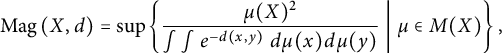 $$ \begin{align} \operatorname{Mag}\left(X,d\right) = \sup \left\{\frac{\mu(X)^2}{\int \int e^{-d(x,y)} \ d\mu(x) d\mu(y)} \mathrel{} \middle| \mathrel{} \mu \in M(X) \right\}, \end{align} $$
where $M(X)$
is the set of finite signed Borel measures on X [Reference Meckes27]. It follows immediately from this definition that
$M(X)$
is the set of finite signed Borel measures on X [Reference Meckes27]. It follows immediately from this definition that $\operatorname {Mag}\left (X,d\right ) \in [1,\infty ]$
, and that magnitude is monotone with respect to set containment for positive definite spaces.
$\operatorname {Mag}\left (X,d\right ) \in [1,\infty ]$
, and that magnitude is monotone with respect to set containment for positive definite spaces.
It is a classical fact that for a normed space E, positive definiteness is equivalent both to the property of being isometrically isomorphic to a subspace of $L_1$
, and being hypermetric (which for general metric spaces is a stronger property than positive definiteness; see, e.g., [Reference Deza and Laurent7, Section 6.1]). We will refer to these spaces as hypermetric normed spaces below. Examples include
$L_1$
, and being hypermetric (which for general metric spaces is a stronger property than positive definiteness; see, e.g., [Reference Deza and Laurent7, Section 6.1]). We will refer to these spaces as hypermetric normed spaces below. Examples include $\ell _p^n = (\mathbb {R}^n, \left \Vert \cdot \right \Vert {}_p)$
for
$\ell _p^n = (\mathbb {R}^n, \left \Vert \cdot \right \Vert {}_p)$
for $1 \le p \le 2$
, in particular
$1 \le p \le 2$
, in particular $\ell _2^n$
, which is
$\ell _2^n$
, which is $\mathbb {R}^n$
with its usual Euclidean norm.
$\mathbb {R}^n$
with its usual Euclidean norm.
Let $\mathcal {K}^n$
be the class of compact, convex subsets of
$\mathcal {K}^n$
be the class of compact, convex subsets of $\mathbb {R}^n$
, equipped with the Hausdorff distance. Recall that a convex valuation on
$\mathbb {R}^n$
, equipped with the Hausdorff distance. Recall that a convex valuation on $\mathbb {R}^n$
is a function
$\mathbb {R}^n$
is a function $V: \mathcal {K}^n \to \mathbb {R}$
such that
$V: \mathcal {K}^n \to \mathbb {R}$
such that
 $$ \begin{align} V(K \cup L) = V(K) + V(L) - V(K\cap L), \end{align} $$
whenever $K, L, K \cup L \subseteq \mathcal {K}^n$
. A convex valuation V is said to be m-homogeneous for
$K, L, K \cup L \subseteq \mathcal {K}^n$
. A convex valuation V is said to be m-homogeneous for $m \in \mathbb {N}$
if
$m \in \mathbb {N}$
if $V(t K) = t^m V(K)$
for every
$V(t K) = t^m V(K)$
for every $K \in \mathcal {K}^n$
and
$K \in \mathcal {K}^n$
and $t>0$
.
$t>0$
.
A consequence of Hadwiger’s classical theorem (see, e.g., [Reference Klain and Rota16, Reference Schneider33, Reference Schneider and Weil34]) is that up to scalar multiples, there is a unique continuous, m-homogeneous, rigid motion-invariant convex valuation $V_m$
on
$V_m$
on $\mathbb {R}^n$
for each
$\mathbb {R}^n$
for each $0 \le m \le n$
. With an appropriate normalization
$0 \le m \le n$
. With an appropriate normalization $V_m(K) = \operatorname {\mathrm {vol}}_m(K)$
whenever
$V_m(K) = \operatorname {\mathrm {vol}}_m(K)$
whenever $K \in \mathcal {K}^n$
is m-dimensional and
$K \in \mathcal {K}^n$
is m-dimensional and $V_m$
is then called the
$V_m$
is then called the $m^{\mathrm {th}}$
intrinsic volume. These quantities, under various normalization and indexing conventions, play a central role in integral geometry.
$m^{\mathrm {th}}$
intrinsic volume. These quantities, under various normalization and indexing conventions, play a central role in integral geometry.
There are multiple natural choices for the normalization of the volume (i.e., Lebesgue measure) on a finite-dimensional normed space E. For the purposes of integral geometry, it turns out that the most convenient normalization is the Holmes–Thompson volume (see, e.g., pages 207–209 of [Reference Schneider and Weil34] for discussion and references). If E is identified with $(\mathbb {R}^n, \left \Vert \cdot \right \Vert )$
and
$(\mathbb {R}^n, \left \Vert \cdot \right \Vert )$
and $\mathbb {R}^n$
is also given its usual Euclidean structure, then the Holmes–Thompson volume of
$\mathbb {R}^n$
is also given its usual Euclidean structure, then the Holmes–Thompson volume of $A \subseteq E$
is given, up to a factor depending only on n, by
$A \subseteq E$
is given, up to a factor depending only on n, by
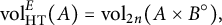 $$ \begin{align} \operatorname{\mathrm{vol}}_{\mathrm{HT}}^E(A) = \operatorname{\mathrm{vol}}_{2n}(A \times B^{\circ}), \end{align} $$
where B is the unit ball of E, $ B^{\circ} = \left\{y \in \mathbb{R}^n \mathrel{} \middle| \mathrel{} \left\langle x, y \right\rangle \le 1 \text{ for every } x \in B \right\} $
is its polar body, and
$ B^{\circ} = \left\{y \in \mathbb{R}^n \mathrel{} \middle| \mathrel{} \left\langle x, y \right\rangle \le 1 \text{ for every } x \in B \right\} $
is its polar body, and $\operatorname {\mathrm {vol}}_{2n}$
is the standard Liouville volume on
$\operatorname {\mathrm {vol}}_{2n}$
is the standard Liouville volume on $\mathbb {R}^n \times (\mathbb {R}^n)^*$
(equal to the usual normalization of Lebesgue measure on
$\mathbb {R}^n \times (\mathbb {R}^n)^*$
(equal to the usual normalization of Lebesgue measure on $\mathbb {R}^{2n}$
under the standard identification
$\mathbb {R}^{2n}$
under the standard identification $(\mathbb {R}^n)^* \cong \mathbb {R}^n$
). The Holmes–Thompson volume is invariant under linear changes of coordinates, and thus independent of the precise identification of E with
$(\mathbb {R}^n)^* \cong \mathbb {R}^n$
). The Holmes–Thompson volume is invariant under linear changes of coordinates, and thus independent of the precise identification of E with $\mathbb {R}^n$
or Euclidean structure. If
$\mathbb {R}^n$
or Euclidean structure. If $F \subseteq E$
is an affine subspace, then we further define
$F \subseteq E$
is an affine subspace, then we further define $\operatorname {\mathrm {vol}}_{\mathrm {HT}}^F(A) = \operatorname {\mathrm {vol}}_{\mathrm {HT}}^{F_0}(A_0)$
for
$\operatorname {\mathrm {vol}}_{\mathrm {HT}}^F(A) = \operatorname {\mathrm {vol}}_{\mathrm {HT}}^{F_0}(A_0)$
for $A \subseteq F$
, where
$A \subseteq F$
, where $F_0$
is the linear subspace of E which is parallel to F and
$F_0$
is the linear subspace of E which is parallel to F and $A_0$
is a translate of A lying in
$A_0$
is a translate of A lying in $F_0$
. (The definition can be further extended to Finsler manifolds, but we will not make use of that level of generality here.)
$F_0$
. (The definition can be further extended to Finsler manifolds, but we will not make use of that level of generality here.)
With the normalization defined by (1.3),
 $$ \begin{align} \operatorname{\mathrm{vol}}_{\mathrm{HT}}^{\ell_2^n}(A) = \operatorname{\mathrm{vol}}_{2n} (A \times B_2^n) = \omega_n \operatorname{\mathrm{vol}}_n(A) \end{align} $$
and
 $$ \begin{align} \operatorname{\mathrm{vol}}_{\mathrm{HT}}^{\ell_1^n}(A) = \operatorname{\mathrm{vol}}_{2n} (A \times B_{\infty}^n) = 2^n \operatorname{\mathrm{vol}}_n(A). \end{align} $$
Here and below, $B_p^n$
denotes the unit ball of
$B_p^n$
denotes the unit ball of $\ell _p^n$
for
$\ell _p^n$
for $1 \le p \le \infty $
and
$1 \le p \le \infty $
and $\omega _n = \operatorname {\mathrm {vol}}_n(B_2^n)$
. In contrast to this, it is standard practice to introduce a factor of
$\omega _n = \operatorname {\mathrm {vol}}_n(B_2^n)$
. In contrast to this, it is standard practice to introduce a factor of $\omega _n^{-1}$
in the definition (1.3) of
$\omega _n^{-1}$
in the definition (1.3) of $\operatorname {\mathrm {vol}}_{\mathrm {HT}}^E$
in order to force the equality
$\operatorname {\mathrm {vol}}_{\mathrm {HT}}^E$
in order to force the equality $\operatorname {\mathrm {vol}}_{\mathrm {HT}}^{\ell _2^n} = \operatorname {\mathrm {vol}}_n$
. This convention reflects the central role of the Euclidean space
$\operatorname {\mathrm {vol}}_{\mathrm {HT}}^{\ell _2^n} = \operatorname {\mathrm {vol}}_n$
. This convention reflects the central role of the Euclidean space $\ell _2^n$
in integral geometry. However, in the theory of magnitude,
$\ell _2^n$
in integral geometry. However, in the theory of magnitude, $\ell _1^n$
plays a more central role, and the convention adopted above is more convenient for the statement and proof of our main result.
$\ell _1^n$
plays a more central role, and the convention adopted above is more convenient for the statement and proof of our main result.
The following partial analog of Hadwiger’s theorem for normed spaces is proved in [Reference Schneider32, Reference Schneider and Wieacker35], although it is not given a self-contained statement.
Proposition 1.1 Let $E = (\mathbb {R}^n, \left \Vert \cdot \right \Vert )$
be a finite-dimensional hypermetric normed space. For each
$E = (\mathbb {R}^n, \left \Vert \cdot \right \Vert )$
be a finite-dimensional hypermetric normed space. For each $1 \le m \le n,$
there is a unique even, continuous, m-homogeneous, translation-invariant convex valuation
$1 \le m \le n,$
there is a unique even, continuous, m-homogeneous, translation-invariant convex valuation $\mu ^E_m$
such that
$\mu ^E_m$
such that $\mu ^E_m(K) = \operatorname {\mathrm {vol}}_{\mathrm {HT}}^F(K)$
whenever
$\mu ^E_m(K) = \operatorname {\mathrm {vol}}_{\mathrm {HT}}^F(K)$
whenever $K \in \mathcal {K}^n$
is m-dimensional and
$K \in \mathcal {K}^n$
is m-dimensional and $F \subseteq E$
is the affine subspace spanned by K.
$F \subseteq E$
is the affine subspace spanned by K.
As discussed in the introduction of [Reference Faifman and Wannerer8], results in [Reference Álvarez Paiva and Fernandes2, Reference Bernig5] imply that Proposition 1.1 holds for certain more general normed spaces. However, it is also shown in [Reference Schneider32] that the valuations $\mu ^E_m$
necessarily have some pathological properties (in particular, failure of monotonicity) if E is not hypermetric.
$\mu ^E_m$
necessarily have some pathological properties (in particular, failure of monotonicity) if E is not hypermetric.
We set $\mu ^E_0 = 1$
. The valuations
$\mu ^E_0 = 1$
. The valuations $\mu ^E_m$
for
$\mu ^E_m$
for $0 \le m \le n$
are referred to as the Holmes–Thompson intrinsic volumes on E. Note that with our normalization convention,
$0 \le m \le n$
are referred to as the Holmes–Thompson intrinsic volumes on E. Note that with our normalization convention, $\mu _m^{\ell _2^n} = \omega _m V_m$
by (1.4). We will denote by
$\mu _m^{\ell _2^n} = \omega _m V_m$
by (1.4). We will denote by $\widetilde {\mu }_m^E = \omega _m^{-1} \mu _m^E$
the usual normalization of the Holmes–Thompson intrinsic volumes, so that
$\widetilde {\mu }_m^E = \omega _m^{-1} \mu _m^E$
the usual normalization of the Holmes–Thompson intrinsic volumes, so that $\widetilde {\mu }_m^{\ell _2^n} = V_m$
.
$\widetilde {\mu }_m^{\ell _2^n} = V_m$
.
We are now ready to state the main theorem of this paper.
Theorem 1.2 Suppose that $E = (\mathbb {R}^n, \left \Vert \cdot \right \Vert )$
is a hypermetric normed space, and let
$E = (\mathbb {R}^n, \left \Vert \cdot \right \Vert )$
is a hypermetric normed space, and let $K \in \mathcal {K}^n$
. Then,
$K \in \mathcal {K}^n$
. Then,
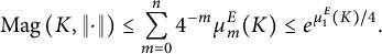 $$\begin{align*}\operatorname{Mag}\left(K, \left\Vert \cdot \right\Vert\right) \le \sum_{m=0}^n 4^{-m} \mu_m^E(K) \le e^{\mu_1^E(K) / 4}. \end{align*}$$
For reference, in terms of the the usual convention for Holmes–Thompson intrinsic volumes, the conclusion of Theorem 1.2 states that
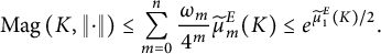 $$\begin{align*}\operatorname{Mag}\left(K, \left\Vert \cdot \right\Vert\right) \le \sum_{m=0}^n \frac{\omega_m}{4^m} \widetilde{\mu}_m^E(K) \le e^{\widetilde{\mu}_1^E(K) / 2}. \end{align*}$$
Theorem 1.2 will be deduced from [Reference Leinster and Meckes22, Theorem 4.6], stated as Theorem 2.1, which is essentially the special case of Theorem 1.2 for $E = \ell _1^n$
. The case of
$E = \ell _1^n$
. The case of $E = \ell _2^n$
was previously deduced from Theorem 2.1 in [Reference Meckes29].
$E = \ell _2^n$
was previously deduced from Theorem 2.1 in [Reference Meckes29].
In Sections 3 and 4, we will combine the upper bound from Theorem 1.2 with easy lower bounds on magnitude to obtain new proofs of results in convex geometry which are not obviously related to magnitude. In the rest of this section, we will state some immediate consequences of Theorem 1.2 about magnitude itself, and in particular for the behavior of the magnitude function $t \mapsto \operatorname {Mag}\left (tK, \left \Vert \cdot \right \Vert \right )$
when
$t \mapsto \operatorname {Mag}\left (tK, \left \Vert \cdot \right \Vert \right )$
when $t \to 0$
. In contrast to this, in Section 3, we will consider the limit of the magnitude function as
$t \to 0$
. In contrast to this, in Section 3, we will consider the limit of the magnitude function as $t \to \infty $
, and in Section 4, we will use a specific finite value of t. This demonstrates that the upper bound in Theorem 1.2, although not necessarily sharp at any value of
$t \to \infty $
, and in Section 4, we will use a specific finite value of t. This demonstrates that the upper bound in Theorem 1.2, although not necessarily sharp at any value of $t> 0$
, is strong enough to yield useful consequences over the entire range of rescalings of K.
$t> 0$
, is strong enough to yield useful consequences over the entire range of rescalings of K.
Our first consequence of Theorem 1.2 is already known. It follows by applying the theorem to the convex hull of X, using the monotonicity of magnitude.
Corollary 1.3 If $E = (\mathbb {R}^n, \left \Vert \cdot \right \Vert )$
is a finite-dimensional hypermetric normed space and
$E = (\mathbb {R}^n, \left \Vert \cdot \right \Vert )$
is a finite-dimensional hypermetric normed space and $X \subseteq E$
is compact, then
$X \subseteq E$
is compact, then $\operatorname {Mag}\left (X, \left \Vert \cdot \right \Vert \right ) < \infty $
, and
$\operatorname {Mag}\left (X, \left \Vert \cdot \right \Vert \right ) < \infty $
, and
 $$\begin{align*}\lim_{t\to 0^+} \operatorname{Mag}\left(tX, \left\Vert \cdot \right\Vert\right) = 1. \end{align*}$$
The finiteness statement in Corollary 1.3 was first proved in this generality in [Reference Leinster and Meckes22, Proposition 4.13] using Fourier analysis. In the recent paper [Reference Leinster and Meckes23], a different proof was given of the finiteness statement which also yielded the limit statement (called the one-point property in [Reference Leinster and Meckes23]). Like the proof of Theorem 1.2, the proof of Corollary 1.3 given in [Reference Leinster and Meckes23] is based on [Reference Leinster and Meckes22, Theorem 4.6].
Theorem 1.2 allows Corollary 1.3 to be generalized to certain infinite-dimensional sets. If $K \subseteq L_1$
is compact and convex, we define
$K \subseteq L_1$
is compact and convex, we define
 $$\begin{align*}\mu_1^{L_1}(K) = \sup\left\{\mu_1^F(K\cap F) \mathrel{} \middle| \mathrel{} F\subseteq L_1 \text{ is a finite-dimensional affine subspace} \right\}. \end{align*}$$
This definition is natural for subsets of $L_1$
since the Holmes–Thompson intrinsic volumes are monotone with respect to set containment in hypermetric normed spaces (and in fact, only in the hypermetric case [Reference Schneider32]). Together with the facts that magnitude is monotone and lower semicontinuous for compact positive definite spaces [Reference Meckes27, Theorem 2.6], Theorem 1.2 yields the following.
$L_1$
since the Holmes–Thompson intrinsic volumes are monotone with respect to set containment in hypermetric normed spaces (and in fact, only in the hypermetric case [Reference Schneider32]). Together with the facts that magnitude is monotone and lower semicontinuous for compact positive definite spaces [Reference Meckes27, Theorem 2.6], Theorem 1.2 yields the following.
Corollary 1.4 If $X \subseteq L_1$
is compact and
$X \subseteq L_1$
is compact and $\mu _1^{L_1}(\operatorname {\mathrm {conv}} X) < \infty $
, then
$\mu _1^{L_1}(\operatorname {\mathrm {conv}} X) < \infty $
, then $\operatorname {Mag}\left (X, \left \Vert \cdot \right \Vert {}_1\right ) < \infty $
, and
$\operatorname {Mag}\left (X, \left \Vert \cdot \right \Vert {}_1\right ) < \infty $
, and
 $$\begin{align*}\lim_{t\to 0^+} \operatorname{Mag}\left(tX, \left\Vert \cdot \right\Vert{}_1\right) = 1. \end{align*}$$
A version of Corollary 1.4 was proved in Corollaries 2 and 3 of [Reference Meckes29] for subsets of a Hilbert space, where the relevant class of sets are known as GB-bodies. Since a separable Hilbert space embeds isometrically in $L_1$
, Corollary 1.4 generalizes those results. The following conjecture is motivated by both Corollary 1.4 and the proof of [Reference Leinster and Meckes23, Theorem 2.1], which gives the first known example of a compact positive definite metric space with infinite magnitude.
$L_1$
, Corollary 1.4 generalizes those results. The following conjecture is motivated by both Corollary 1.4 and the proof of [Reference Leinster and Meckes23, Theorem 2.1], which gives the first known example of a compact positive definite metric space with infinite magnitude.
Conjecture 1.5 Suppose that $K \subseteq L_1$
is compact and convex. Then
$K \subseteq L_1$
is compact and convex. Then $\operatorname {Mag}\left (K, \left \Vert \cdot \right \Vert {}_1\right ) < \infty $
if and only if
$\operatorname {Mag}\left (K, \left \Vert \cdot \right \Vert {}_1\right ) < \infty $
if and only if $\mu _1^{L_1}(K) < \infty $
.
$\mu _1^{L_1}(K) < \infty $
.
The one-point property can be sharpened to the following first-order bound on the magnitude function for small t, generalizing part of [Reference Meckes29, Corollary 6] for the Euclidean case.
Corollary 1.6 Suppose that $E = (\mathbb {R}^n, \left \Vert \cdot \right \Vert )$
is a hypermetric normed space, and let
$E = (\mathbb {R}^n, \left \Vert \cdot \right \Vert )$
is a hypermetric normed space, and let $K \in \mathcal {K}^n$
. Then
$K \in \mathcal {K}^n$
. Then
 $$\begin{align*}\limsup_{t\to 0^+} \frac{\operatorname{Mag}\left(tK, \left\Vert \cdot \right\Vert\right) - 1}{t} \le \frac{1}{4} \mu_1^E(K). \end{align*}$$
The following conjecture, which generalizes [Reference Meckes29, Conjecture 5], posits that the upper bounds in Theorem 1.2 are sharp to first order for small convex sets.
Conjecture 1.7 Suppose that $E = (\mathbb {R}^n, \left \Vert \cdot \right \Vert )$
is a hypermetric normed space, and let
$E = (\mathbb {R}^n, \left \Vert \cdot \right \Vert )$
is a hypermetric normed space, and let $K \in \mathcal {K}^n$
. Then
$K \in \mathcal {K}^n$
. Then
 $$\begin{align*}\lim_{t \to 0^+} \frac{\operatorname{Mag}\left(tK, \left\Vert \cdot \right\Vert\right) - 1}{t} = \frac{1}{4} \mu_1^E(K). \end{align*}$$
When $E = \ell _1^n$
, Conjecture 1.7 holds whenever K has nonempty interior, by Theorem 2.1. When
$E = \ell _1^n$
, Conjecture 1.7 holds whenever K has nonempty interior, by Theorem 2.1. When $E = \ell _2^n$
the conjecture holds if n is odd and
$E = \ell _2^n$
the conjecture holds if n is odd and $K = B_2^n$
, by [Reference Meckes29, Theorem 4]. In all other cases, the conjecture is open, although the results of [Reference Gimperlein and Goffeng9] imply that if
$K = B_2^n$
, by [Reference Meckes29, Theorem 4]. In all other cases, the conjecture is open, although the results of [Reference Gimperlein and Goffeng9] imply that if $E = \ell _2^n$
, n is odd, and K has smooth boundary, then the limit exists.
$E = \ell _2^n$
, n is odd, and K has smooth boundary, then the limit exists.
The rest of this paper is organized as follows: in Section 2, we will prove Theorem 1.2. In Sections 3 and 4, we will see how Theorem 1.2 quickly yields, respectively, Mahler’s conjecture for zonoids and Sudakov’s minoration inequality. Finally, in Section 5, we will make some remarks about Leinster’s $\ell _1$
integral geometry, which underlies Theorem 2.1, and its relationships to both the theory of Holmes–Thompson intrinsic volumes and the Wills functional.
$\ell _1$
integral geometry, which underlies Theorem 2.1, and its relationships to both the theory of Holmes–Thompson intrinsic volumes and the Wills functional.
2 Proof of Theorem 1.2
To state the theorem on which the proof of Theorem 1.2 is based, we first define some additional notation. Following [Reference Leinster18], for $0 \le m \le n$
, we define the
$0 \le m \le n$
, we define the $\pmb{\ell}_1$
intrinsic volumes of
$\pmb{\ell}_1$
intrinsic volumes of $K \in \mathcal {K}^n$
by
$K \in \mathcal {K}^n$
by
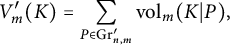 $$\begin{align*}V_m'(K) = \sum_{P \in \mathrm{Gr}^{\prime}_{n,m}} \operatorname{\mathrm{vol}}_m(K\vert P), \end{align*}$$
where $\mathrm {Gr}^{\prime }_{n,m}$
denotes the set of m-dimensional coordinate subspaces of
$\mathrm {Gr}^{\prime }_{n,m}$
denotes the set of m-dimensional coordinate subspaces of $\mathbb {R}^n$
and
$\mathbb {R}^n$
and $K \vert P$
denotes the orthogonal projection of K onto P. (The natural class of sets to consider here is actually larger than convex bodies, a point that we will return to in Section 5.) Note that if K lies in a d-dimensional subspace of
$K \vert P$
denotes the orthogonal projection of K onto P. (The natural class of sets to consider here is actually larger than convex bodies, a point that we will return to in Section 5.) Note that if K lies in a d-dimensional subspace of $\ell _1^n$
, then
$\ell _1^n$
, then $V_m'(K) = 0$
for
$V_m'(K) = 0$
for $m> d$
. It follows that
$m> d$
. It follows that
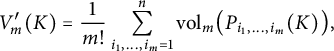 $$\begin{align*}V_m'(K) = \frac{1}{m!} \sum_{i_1, \dots, i_m = 1}^n \operatorname{\mathrm{vol}}_m \bigl(P_{i_1, \dots, i_m} (K)\bigr), \end{align*}$$
where $P_{i_1, \dots , i_m}:\mathbb {R}^n \to \mathbb {R}^m$
is the linear map represented by the matrix whose rows are the standard basis vectors
$P_{i_1, \dots , i_m}:\mathbb {R}^n \to \mathbb {R}^m$
is the linear map represented by the matrix whose rows are the standard basis vectors $e_{i_1}, \dots , e_{i_m} \in \mathbb {R}^n$
.
$e_{i_1}, \dots , e_{i_m} \in \mathbb {R}^n$
.
The following result is part of Theorem 4.6 of [Reference Leinster and Meckes22].
Theorem 2.1 If $K \in \mathcal {K}^n$
, then
$K \in \mathcal {K}^n$
, then
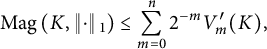 $$\begin{align*}\operatorname{Mag}\left(K, \left\Vert \cdot \right\Vert{}_1\right) \le \sum_{m=0}^n 2^{-m} V_m'(K), \end{align*}$$
with equality when K has nonempty interior.
To deduce Theorem 1.2 from Theorem 2.1, we approximate a hypermetric normed space E by a sequence of n-dimensional subspaces $E_N \subseteq \ell _1^N$
. To do this, we use the following fact, which goes back to Lévy (see, e.g., [Reference Koldobsky17, Section 6.1]).
$E_N \subseteq \ell _1^N$
. To do this, we use the following fact, which goes back to Lévy (see, e.g., [Reference Koldobsky17, Section 6.1]).
Proposition 2.2 A finite-dimensional normed space $E = (\mathbb {R}^n, \left \Vert \cdot \right \Vert )$
is hypermetric if and only if, there exists an even nonnegative measure
$E = (\mathbb {R}^n, \left \Vert \cdot \right \Vert )$
is hypermetric if and only if, there exists an even nonnegative measure $\rho $
on
$\rho $
on $S^{n-1}$
such that
$S^{n-1}$
such that
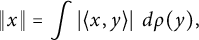 $$\begin{align*}\left\Vert x \right\Vert = \int \left\vert \left\langle x, y \right\rangle \right\vert \ d\rho(y), \end{align*}$$
for all $x \in \mathbb {R}^n$
.
$x \in \mathbb {R}^n$
.
From the perspective of convex geometry, Proposition 2.2 implies that E is hypermetric if and only if $B^{\circ }$
, the polar body of the unit ball of E, is a zonoid (see [Reference Schneider33, Theorem 3.5.3]). In that setting
$B^{\circ }$
, the polar body of the unit ball of E, is a zonoid (see [Reference Schneider33, Theorem 3.5.3]). In that setting $\rho $
is referred to as the generating measure of
$\rho $
is referred to as the generating measure of $B^{\circ }$
; we will also refer to it as the generating measure for E. In [Reference Schneider and Wieacker35], Schneider and Wieacker investigated Holmes–Thompson intrinsic volumes for hypermetric normed spaces with the help of generating measures. We will use the following expression they derived (see [Reference Schneider and Wieacker35, formula (64)]).
$B^{\circ }$
; we will also refer to it as the generating measure for E. In [Reference Schneider and Wieacker35], Schneider and Wieacker investigated Holmes–Thompson intrinsic volumes for hypermetric normed spaces with the help of generating measures. We will use the following expression they derived (see [Reference Schneider and Wieacker35, formula (64)]).
Proposition 2.3 Suppose that $E = (\mathbb {R}^n, \left \Vert \cdot \right \Vert )$
is a hypermetric normed space with generating measure
$E = (\mathbb {R}^n, \left \Vert \cdot \right \Vert )$
is a hypermetric normed space with generating measure $\rho $
. Then
$\rho $
. Then
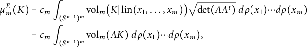 $$ \begin{align*} \mu_m^E(K) & = c_m \int_{(S^{n-1})^m} \operatorname{\mathrm{vol}}_m \bigl(K \vert \operatorname{lin}(x_1, \dots, x_m)\bigr) \sqrt{\det (A A^t)} \ d\rho(x_1) \cdots d\rho(x_m) \\ & = c_m \int_{(S^{n-1})^m} \operatorname{\mathrm{vol}}_m (A K) \ d\rho(x_1) \cdots d\rho(x_m), \end{align*} $$
where $c_m$
depends only on m. Here,
$c_m$
depends only on m. Here, $\operatorname {lin}(x_1,\dots x_n)$
denotes the linear span of
$\operatorname {lin}(x_1,\dots x_n)$
denotes the linear span of $x_1,\dots , x_m \in \mathbb {R}^n$
and A is the
$x_1,\dots , x_m \in \mathbb {R}^n$
and A is the $m \times n$
matrix with rows
$m \times n$
matrix with rows $x_1, \dots , x_m$
.
$x_1, \dots , x_m$
.
Since we are using a different normalization convention than [Reference Schneider and Wieacker35], the value of $c_m$
here differs from the one stated in [Reference Schneider and Wieacker35]. The proof of the following corollary shows that for our normalization,
$c_m$
here differs from the one stated in [Reference Schneider and Wieacker35]. The proof of the following corollary shows that for our normalization, $c_m = \frac {2^m}{m!}$
.
$c_m = \frac {2^m}{m!}$
.
Corollary 2.4 For $K \in \mathcal {K}^n$
, μ
m
ℓ
1
n
(K) = 2
m
V
m
′(K).
$K \in \mathcal {K}^n$
, μ
m
ℓ
1
n
(K) = 2
m
V
m
′(K).
Proof The generating measure for $\ell _1^n$
is
$\ell _1^n$
is $\rho = \frac {1}{2} \sum _{i=1}^n (\delta _{e_i} + \delta _{-e_i})$
. If
$\rho = \frac {1}{2} \sum _{i=1}^n (\delta _{e_i} + \delta _{-e_i})$
. If $x_1, \dots , x_m \in \{\pm e_1, \dots , \pm e_n\}$
, then
$x_1, \dots , x_m \in \{\pm e_1, \dots , \pm e_n\}$
, then $\sqrt {\det (A A^t)} = 1$
if
$\sqrt {\det (A A^t)} = 1$
if $\operatorname {lin}(x_1, \dots , x_m)$
is m-dimensional, and is
$\operatorname {lin}(x_1, \dots , x_m)$
is m-dimensional, and is $0$
otherwise. Proposition 2.3 therefore implies that
$0$
otherwise. Proposition 2.3 therefore implies that
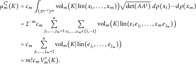 $$ \begin{align*} \mu_m^{\ell_1^n}(K) & = c_m \int_{(S^{n-1})^m} \operatorname{\mathrm{vol}}_m \bigl(K \vert \operatorname{lin}(x_1, \dots, x_m)\bigr) \sqrt{\det (A A^t)} \ d\rho(x_1) \cdots d\rho(x_m) \\ & = 2^{-m} c_m \sum_{j_1, \dots, j_m = 1}^n \sum_{\varepsilon_1, \dots, \varepsilon_m \in \{1, -1\}} \operatorname{\mathrm{vol}}_m \bigl(K \vert \operatorname{lin}(\varepsilon_1 e_{j_1}, \dots, \varepsilon_m e_{j_m})\bigr) \\ & = c_m \sum_{j_1, \dots, j_m = 1}^n \operatorname{\mathrm{vol}}_m \bigl(K \vert \operatorname{lin}(e_{j_1}, \dots, e_{j_m})\bigr) \\ & = m! c_m V_m'(K). \end{align*} $$
Now, if $E \subseteq \ell _1^n$
is an m-dimensional coordinate subspace, then E is isometrically isomorphic to
$E \subseteq \ell _1^n$
is an m-dimensional coordinate subspace, then E is isometrically isomorphic to $\ell _1^m$
, and when
$\ell _1^m$
, and when $K \subseteq E$
we have
$K \subseteq E$
we have
 $$\begin{align*}\mu_m^{\ell_1^n}(K) = \operatorname{\mathrm{vol}}_{\mathrm{HT}}^E(K) = 2^m \operatorname{\mathrm{vol}}_m(K) = 2^m V_m'(K) \end{align*}$$
by (1.5) and [Reference Leinster18, Lemma 5.2], and so $c_m = \frac {2^m}{m!}$
.
$c_m = \frac {2^m}{m!}$
.
Corollary 2.4 shows in particular that when $E = \ell _1^n$
, the first inequality in Theorem 1.2 reduces to Theorem 2.1. It also implies the following generalization of [Reference Leinster18, Lemma 5.2].
$E = \ell _1^n$
, the first inequality in Theorem 1.2 reduces to Theorem 2.1. It also implies the following generalization of [Reference Leinster18, Lemma 5.2].
Corollary 2.5 If $K \in \mathcal {K}^n$
lies in an m-dimensional subspace
$K \in \mathcal {K}^n$
lies in an m-dimensional subspace $E \subseteq \mathbb {R}^n$
, then
$E \subseteq \mathbb {R}^n$
, then
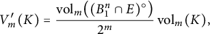 $$\begin{align*}V_m'(K) = \frac{\operatorname{\mathrm{vol}}_m\bigl( (B_1^n \cap E)^{\circ}\bigr)}{2^m} \operatorname{\mathrm{vol}}_m(K), \end{align*}$$
where the polar body $(B_1^n \cap E)^{\circ }$
is considered in the subspace E.
$(B_1^n \cap E)^{\circ }$
is considered in the subspace E.
For the second inequality in Theorem 1.2, we will need the following generalization of [Reference Leinster and Meckes23, Lemma 3.2].
Lemma 2.6 If $E = (\mathbb {R}^n, \left \Vert \cdot \right \Vert )$
is a hypermetric normed space and
$E = (\mathbb {R}^n, \left \Vert \cdot \right \Vert )$
is a hypermetric normed space and $K \in \mathcal {K}^n$
, then
$K \in \mathcal {K}^n$
, then $\mu _{i+j}^E(K) \le \frac {i! j!}{(i+j)!} \mu _i^E(K) \mu _j^E(K)$
for all
$\mu _{i+j}^E(K) \le \frac {i! j!}{(i+j)!} \mu _i^E(K) \mu _j^E(K)$
for all $i, j \ge 0$
. Consequently,
$i, j \ge 0$
. Consequently, $\mu _m^E(K) \le \frac {1}{m!} (\mu _1^E(K))^m$
for each
$\mu _m^E(K) \le \frac {1}{m!} (\mu _1^E(K))^m$
for each $1\le m \le n$
.
$1\le m \le n$
.
Proof Let $x_1, \dots , x_{i+j} \in \mathbb {R}^n$
. Writing A for the matrix with rows
$x_1, \dots , x_{i+j} \in \mathbb {R}^n$
. Writing A for the matrix with rows $x_1, \dots , x_{i+j}$
,
$x_1, \dots , x_{i+j}$
, $A_1$
for the matrix with rows
$A_1$
for the matrix with rows $x_1, \dots , x_i$
, and
$x_1, \dots , x_i$
, and $A_2$
for the matrix with rows
$A_2$
for the matrix with rows $x_{i+1}, \dots , x_j$
, we have
$x_{i+1}, \dots , x_j$
, we have $A K \subseteq A_1 K \times A_2 K$
. Proposition 2.3 then implies that
$A K \subseteq A_1 K \times A_2 K$
. Proposition 2.3 then implies that
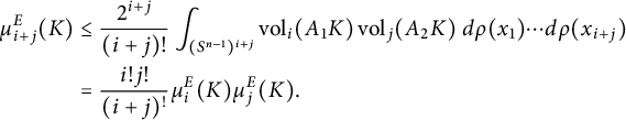 $$ \begin{align*} \mu_{i+j}^E(K) & \le \frac{2^{i+j}}{(i+j)!} \int_{(S^{n-1})^{i+j}} \operatorname{\mathrm{vol}}_i (A_1 K) \operatorname{\mathrm{vol}}_j(A_2 K) \ d\rho(x_1) \cdots d\rho(x_{i+j}) \\ & = \frac{i! j!}{(i+j)^!} \mu_i^E(K) \mu_j^E(K). \end{align*} $$
This implies in particular that $\mu _{j+1}^E(K) \le \frac {1}{j+1} \mu _1^E(K) \mu _j^E(K)$
for each j, and the second claim now follows by induction.
$\mu _{j+1}^E(K) \le \frac {1}{j+1} \mu _1^E(K) \mu _j^E(K)$
for each j, and the second claim now follows by induction.
We are now ready to prove the main result.
Proof of Theorem 1.2
Let $\rho $
be the generating measure for E. We can approximate
$\rho $
be the generating measure for E. We can approximate $\rho $
by a sequence of discrete measures
$\rho $
by a sequence of discrete measures
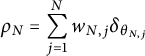 $$\begin{align*}\rho_N = \sum_{j=1}^{N} w_{N,j} \delta_{\theta_{N,j}} \end{align*}$$
with $w_{N,j}> 0$
and
$w_{N,j}> 0$
and $\theta _{N,j} \in S^{n-1}$
. For each
$\theta _{N,j} \in S^{n-1}$
. For each $N,$
we get a seminorm, which for sufficiently large
$N,$
we get a seminorm, which for sufficiently large $N \ge n$
will be a norm, given by
$N \ge n$
will be a norm, given by
 $$\begin{align*}\left\Vert x \right\Vert{}_{E_N} = \int_{S^{n-1}} \left\vert \left\langle x, y \right\rangle \right\vert \ d\rho_N(y) = \sum_{j=1}^m w_{N,j} \left\vert \left\langle x, \theta_{N,j} \right\rangle \right\vert = \sum_{j=1}^N \left\vert \left\langle x, w_{N,j} \theta_{N,j} \right\rangle \right\vert. \end{align*}$$
We write $E_N = (\mathbb {R}^n, \left \Vert \cdot \right \Vert {}_{E_N})$
. Define
$E_N = (\mathbb {R}^n, \left \Vert \cdot \right \Vert {}_{E_N})$
. Define $T_N:\mathbb {R}^N \to \mathbb {R}^n$
by
$T_N:\mathbb {R}^N \to \mathbb {R}^n$
by $T_N(e_j) = w_{N,j} \theta _{N,j}$
. Then
$T_N(e_j) = w_{N,j} \theta _{N,j}$
. Then
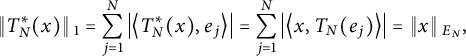 $$\begin{align*}\left\Vert T^*_N(x) \right\Vert{}_1 = \sum_{j=1}^N \left\vert \left\langle T_N^*(x), e_j \right\rangle \right\vert = \sum_{j=1}^N \left\vert \left\langle x, T_N(e_j) \right\rangle \right\vert = \left\Vert x \right\Vert{}_{E_N}, \end{align*}$$
so $T_N^*$
is an isometric embedding of
$T_N^*$
is an isometric embedding of $E_N$
into
$E_N$
into $\ell _1^N$
.
$\ell _1^N$
.
We have
 $$\begin{align*}\left\Vert x \right\Vert{}_{E_N} = \int_{S^{n-1}} \left\vert \left\langle x, y \right\rangle \right\vert \ d\rho_N(y) \xrightarrow{N \to \infty} \int_{S^{n-1}} \left\vert \left\langle x, y \right\rangle \right\vert \ d\rho(y) = \left\Vert x \right\Vert. \end{align*}$$
This implies that $(K, \left \Vert \cdot \right \Vert {}_{E_N}) \to (K, \left \Vert \cdot \right \Vert )$
in the Gromov–Hausdorff metric (see [Reference Gromov13, Section 3.A]). Since magnitude is lower semicontinuous with respect to the Gromov–Hausdorff metric on the class of compact positive definite metric spaces [Reference Meckes27, Theorem 2.6], it follows that
$(K, \left \Vert \cdot \right \Vert {}_{E_N}) \to (K, \left \Vert \cdot \right \Vert )$
in the Gromov–Hausdorff metric (see [Reference Gromov13, Section 3.A]). Since magnitude is lower semicontinuous with respect to the Gromov–Hausdorff metric on the class of compact positive definite metric spaces [Reference Meckes27, Theorem 2.6], it follows that
 $$ \begin{align} \operatorname{Mag}\left(K, \left\Vert \cdot \right\Vert\right) \le \liminf_{N \to \infty} \operatorname{Mag}\left(K, \left\Vert \cdot \right\Vert{}_{E_N}\right) = \liminf_{N \to \infty} \operatorname{Mag}\left(T_N^* (K), \left\Vert \cdot \right\Vert{}_1\right). \end{align} $$
Now,
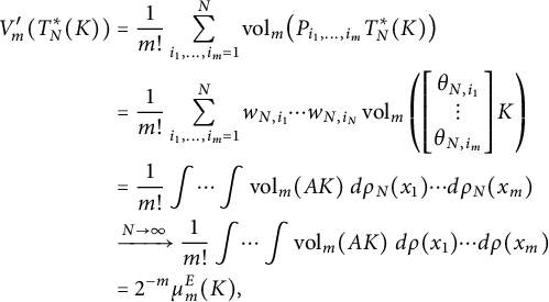 $$ \begin{align} \begin{aligned} V_m'(T_N^*(K)) & = \frac{1}{m!} \sum_{i_1, \dots, i_m = 1}^N \operatorname{\mathrm{vol}}_m \bigl(P_{i_1, \dots, i_m} T_N^*(K) \bigr) \\ & = \frac{1}{m!} \sum_{i_1, \dots, i_m = 1}^N w_{N,i_1} \cdots w_{N,i_N} \operatorname{\mathrm{vol}}_m \left( \begin{bmatrix} \theta_{N,i_1} \\ \vdots \\ \theta_{N,i_m} \end{bmatrix} K \right) \\ & = \frac{1}{m!} \int \dots \int \operatorname{\mathrm{vol}}_m (A K ) \ d\rho_N(x_1) \cdots d\rho_N(x_m) \\ & \xrightarrow{N \to \infty} \frac{1}{m!} \int \dots \int \operatorname{\mathrm{vol}}_m (A K ) \ d\rho(x_1) \cdots d\rho(x_m) \\ & = 2^{-m} \mu_m^{E}(K), \end{aligned} \end{align} $$
where the last equality follows from Proposition 2.3. Here, A as before stands for the matrix with rows $x_1, \dots , x_m$
, and the matrix in the second row has rows
$x_1, \dots , x_m$
, and the matrix in the second row has rows $\theta _{N,i_1}, \dots , \theta _{N,i_m}$
. The first inequality in Theorem 1.2 now follows by combining (2.1), Theorem 2.1, and (2.2). The second inequality then follows by Lemma 2.6.
$\theta _{N,i_1}, \dots , \theta _{N,i_m}$
. The first inequality in Theorem 1.2 now follows by combining (2.1), Theorem 2.1, and (2.2). The second inequality then follows by Lemma 2.6.
3 Application: Mahler’s conjecture for zonoids
In this and the following section, we will see how two important results in convex geometry which make no reference to magnitude quickly follow by combining the upper bound on magnitude from Theorem 1.2 with easy lower bounds.
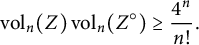
Mahler conjectured in 1939 [Reference Mahler25] that if $K \in \mathcal {K}^n$
is symmetric with nonempty interior, then
$K \in \mathcal {K}^n$
is symmetric with nonempty interior, then
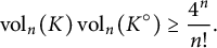 $$\begin{align*}\operatorname{\mathrm{vol}}_n(K) \operatorname{\mathrm{vol}}_n(K^{\circ}) \ge \frac{4^n}{n!}. \end{align*}$$
Equality is attained (nonuniquely) for $K = B_1^n$
or
$K = B_1^n$
or $K = B_{\infty }^n$
. This has been proved in various special cases and in asymptotic forms (see [Reference Iriyeh and Shibata15] for a proof when
$K = B_{\infty }^n$
. This has been proved in various special cases and in asymptotic forms (see [Reference Iriyeh and Shibata15] for a proof when $n=3$
and further references), but the general case remains open.
$n=3$
and further references), but the general case remains open.
In the proof of the following result, we compare the top-order behavior of the first upper bound on magnitude in Theorem 1.2, which is typically not sharp for large convex bodies, with a lower bound that is known to be asymptotically sharp. This comparison immediately implies Mahler’s conjecture for zonoids, first proved in [Reference Reisner30, Reference Reisner31] (see also [Reference Gordon, Meyer and Reisner12]).
Corollary 3.1 If $Z \in \mathcal {K}^n$
is an n-dimensional zonoid, then
$Z \in \mathcal {K}^n$
is an n-dimensional zonoid, then
 $$\begin{align*}\operatorname{\mathrm{vol}}_n(Z) \operatorname{\mathrm{vol}}_n(Z^{\circ}) \ge \frac{4^n}{n!}. \end{align*}$$
Proof Let $E = (\mathbb {R}^n, \left \Vert \cdot \right \Vert )$
be the hypermetric normed space with unit ball
$E = (\mathbb {R}^n, \left \Vert \cdot \right \Vert )$
be the hypermetric normed space with unit ball $B = Z^{\circ }$
. Theorem 1.2 implies that for
$B = Z^{\circ }$
. Theorem 1.2 implies that for $t \to \infty $
,
$t \to \infty $
,
 $$\begin{align*}\operatorname{Mag}\left(t B,\left\Vert \cdot \right\Vert\right) \le 4^{-n} \mu_n^E(B) t^n + O(t^{n-1}) = 4^{-n} \operatorname{\mathrm{vol}}_n(B) \operatorname{\mathrm{vol}}_n(B^{\circ}) t^n + O(t^{n-1}). \end{align*}$$
On the other hand, for each $t> 0,$
we have the lower bound
$t> 0,$
we have the lower bound
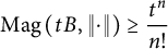 $$\begin{align*}\operatorname{Mag}\left(t B, \left\Vert \cdot \right\Vert\right) \ge \frac{t^n}{n!} \end{align*}$$
(see [Reference Leinster19, Theorem 3.5.6] or [Reference Leinster and Meckes22, Proposition 4.13]). Combining these, we obtain
 $$\begin{align*}\frac{4^n}{n!} \le \operatorname{\mathrm{vol}}_n(B) \operatorname{\mathrm{vol}}_n(B^{\circ}) + O(t^{-1}) = \operatorname{\mathrm{vol}}_n(Z) \operatorname{\mathrm{vol}}_n(Z^{\circ}) + O(t^{-1}), \end{align*}$$
and letting $t \to \infty $
proves the claim.
$t \to \infty $
proves the claim.
Remark Although we considered $\operatorname {Mag}\left (tB, \left \Vert \cdot \right \Vert \right )$
in the above proof for convenience, we could equally well consider
$\operatorname {Mag}\left (tB, \left \Vert \cdot \right \Vert \right )$
in the above proof for convenience, we could equally well consider $\operatorname {Mag}\left (tK, \left \Vert \cdot \right \Vert \right )$
for any n-dimensional convex body K (with the norm still corresponding to
$\operatorname {Mag}\left (tK, \left \Vert \cdot \right \Vert \right )$
for any n-dimensional convex body K (with the norm still corresponding to $B = Z^{\circ }$
) and obtain the same result.
$B = Z^{\circ }$
) and obtain the same result.
4 Application: Sudakov minoration
Our last application of Theorem 1.2 is a new proof of Sudakov’s minoration inequality, which is a key tool in both high-dimensional convex geometry and the theory of Gaussian processes (see, e.g., [Reference Artstein-Avidan, Giannopoulos and Milman3, Reference Talagrand37], respectively). This application uses only the special case of Theorem 1.2 when $E = \ell _2^n$
, proved previously in [Reference Meckes29]. In that case, the first upper bound in Theorem 1.2 can be combined with a stronger counterpart to Lemma 2.6 in Euclidean space to deduce the following sharper version of the second upper bound.
$E = \ell _2^n$
, proved previously in [Reference Meckes29]. In that case, the first upper bound in Theorem 1.2 can be combined with a stronger counterpart to Lemma 2.6 in Euclidean space to deduce the following sharper version of the second upper bound.
Corollary 4.1 If $K \in \mathcal {K}^n$
, then
$K \in \mathcal {K}^n$
, then
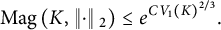 $$\begin{align*}\operatorname{Mag}\left(K, \left\Vert \cdot \right\Vert{}_2\right) \le e^{C V_1(K)^{2/3}}. \end{align*}$$
Throughout this section, c, C, and $C'$
refer to absolute positive constants whose values may differ from one instance to another.
$C'$
refer to absolute positive constants whose values may differ from one instance to another.
Remark Corollary 4.1 can be extended to infinite-dimensional Hilbert spaces, similarly to Corollary 1.4, but for simplicity, we will restrict attention to finite dimensions in this section.
Proof of Corollary 4.1
It was independently shown by Chevet [Reference Chevet6, Lemma 4.2] and McMullen [Reference McMullen26, Theorem 2] that the Alexandrov–Fenchel inequalities imply that $V_m \le \frac {1}{m!} V_1^m$
for every
$V_m \le \frac {1}{m!} V_1^m$
for every $m \ge 1$
. As observed in formula (17) of [Reference Meckes29], Theorem 1.2 then implies that
$m \ge 1$
. As observed in formula (17) of [Reference Meckes29], Theorem 1.2 then implies that
 $$\begin{align*}\operatorname{Mag}\left(K, \left\Vert \cdot \right\Vert{}_2\right) \le \sum_{m=0}^n \frac{\omega_m}{m!} \left(\frac{V_1(K)}{4}\right)^m = \sum_{m=0}^n \frac{1}{\Gamma \bigl(1 + \frac{m}{2}\bigr) m!} \left(\frac{\sqrt{\pi} V_1(K)}{4}\right)^m. \end{align*}$$
We now consider the function
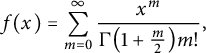 $$\begin{align*}f(x) = \sum_{m=0}^{\infty} \frac{x^m}{\Gamma \bigl(1 + \frac{m}{2}\bigr) m!}, \end{align*}$$
a special case of Wright’s generalized hypergeometric function. We claim that $f(x) \le e^{c x^{2/3}}$
for
$f(x) \le e^{c x^{2/3}}$
for $x> 0$
, which will complete the proof.
$x> 0$
, which will complete the proof.
If $x \le 1$
, then since
$x \le 1$
, then since $\Gamma \bigl (1 + \frac {m}{2}\bigr ) \ge \frac {\sqrt {\pi }}{2}$
for every
$\Gamma \bigl (1 + \frac {m}{2}\bigr ) \ge \frac {\sqrt {\pi }}{2}$
for every $m \ge 0$
, we have
$m \ge 0$
, we have
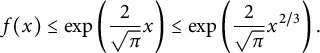 $$\begin{align*}f(x) \le \exp\left(\frac{2}{\sqrt{\pi}} x\right) \le \exp\left(\frac{2}{\sqrt{\pi}} x^{2/3}\right). \end{align*}$$
For $x \ge 1$
, Stirling’s approximation implies that
$x \ge 1$
, Stirling’s approximation implies that
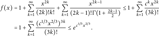 $$ \begin{align*} f(x) & = 1 + \sum_{k=1}^{\infty} \frac{x^{2k}}{(2k)! k!} + \sum_{k=1}^{\infty} \frac{x^{2k-1}}{(2k-1)! \Gamma(1 + \frac{2k-1}{2})} \le 1 + \sum_{k=1}^{\infty} \frac{c^k x^{2k}}{(3k)!} \\ & = 1 + \sum_{k=1}^{\infty} \frac{(c^{1/3} x^{2/3})^{3k}}{(3k)!} \le e^{c^{1/3} x^{2/3}}.\\[-42pt] \end{align*} $$
Since $V_1$
is
$V_1$
is $1$
-homogeneous, Corollary 4.1 is equivalent to the following.
$1$
-homogeneous, Corollary 4.1 is equivalent to the following.
Corollary 4.2 If $K \in \mathcal {K}^n$
, then
$K \in \mathcal {K}^n$
, then
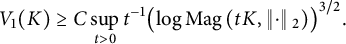 $$\begin{align*}V_1(K) \ge C \sup_{t> 0} t^{-1} \bigl(\log \operatorname{Mag}\left(t K, \left\Vert \cdot \right\Vert{}_2\right)\bigr)^{3/2}. \end{align*}$$
Corollary 4.3 (Sudakov’s minoration inequality)
Let $K \in \mathcal {K}^n$
, and suppose there exist
$K \in \mathcal {K}^n$
, and suppose there exist $x_1, \dots , x_N \in K$
such that
$x_1, \dots , x_N \in K$
such that $\left \Vert x_i - x_j \right \Vert {}_2 \ge \varepsilon $
whenever
$\left \Vert x_i - x_j \right \Vert {}_2 \ge \varepsilon $
whenever $i\neq j$
. Then
$i\neq j$
. Then
 $$\begin{align*}V_1(K) \ge C \varepsilon \sqrt{\log N}. \end{align*}$$
Proof Assume without loss of generality that $N \ge 2$
, and let
$N \ge 2$
, and let $\mu = \sum _{i=1}^N \delta _{x_i}$
. By (1.1),
$\mu = \sum _{i=1}^N \delta _{x_i}$
. By (1.1),
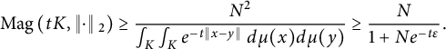 $$\begin{align*}\operatorname{Mag}\left(t K, \left\Vert \cdot \right\Vert{}_2\right) \ge \frac{N^2}{\int_K \int_K e^{-t \left\Vert x-y \right\Vert} \ d\mu(x) d\mu(y)} \ge \frac{N}{1 + N e^{-t \varepsilon}}. \end{align*}$$
If $t = \frac {\log (2N)}{\varepsilon },$
this implies that
$t = \frac {\log (2N)}{\varepsilon },$
this implies that
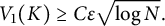
 $\operatorname {Mag}\left (t K, \left \Vert \cdot \right \Vert {}_2\right ) \ge \frac {2}{3} N$
, and so Corollary 4.2 implies that
$\operatorname {Mag}\left (t K, \left \Vert \cdot \right \Vert {}_2\right ) \ge \frac {2}{3} N$
, and so Corollary 4.2 implies that
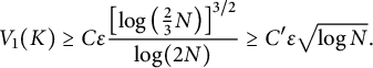 $$\begin{align*}V_1(K) \ge C \varepsilon \frac{\left[\log \left(\frac{2}{3} N \right)\right]^{3/2}}{\log (2N)} \ge C' \varepsilon \sqrt{\log N}. \\[-42pt] \end{align*}$$
Remark If the supremum in our definition (1.1) of magnitude is restricted to positive measures $\mu $
, we obtain a quantity called the maximum diversity of
$\mu $
, we obtain a quantity called the maximum diversity of $(X,d)$
, denoted
$(X,d)$
, denoted $D_{\max }(X,d)$
(see [Reference Leinster and Roff24, Reference Meckes27]). The above proof of Corollary 4.3 shows that
$D_{\max }(X,d)$
(see [Reference Leinster and Roff24, Reference Meckes27]). The above proof of Corollary 4.3 shows that
 $$\begin{align*}\sup_{t> 0} t^{-1} \bigl(\log D_{\max}(t K, \left\Vert \cdot \right\Vert{}_2)\bigr)^{3/2} \ge C \sup_{\varepsilon > 0} \varepsilon \sqrt{\log N(K,\varepsilon)}, \end{align*}$$
where $N(K,\varepsilon )$
is the maximum size of a collection of
$N(K,\varepsilon )$
is the maximum size of a collection of $\varepsilon $
-separated points in K. It can similarly be shown that
$\varepsilon $
-separated points in K. It can similarly be shown that
 $$\begin{align*}\sup_{t> 0} t^{-1} \bigl(\log D_{\max}(t K, \left\Vert \cdot \right\Vert{}_2)\bigr)^{3/2} \le C' \sup_{\varepsilon > 0} \varepsilon \sqrt{\log N(K,\varepsilon)} \end{align*}$$
(cf. the proof of [Reference Meckes28, Theorem 7.1]). It follows that Sudakov’s minoration inequality is equivalent, up to the value of the constant C, to the inequality
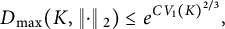 $$\begin{align*}D_{\max}(K, \left\Vert \cdot \right\Vert{}_2) \le e^{C V_1(K)^{2/3}}, \end{align*}$$
a weaker counterpart of Corollary 4.1.
This observation suggests trying to prove sharper lower bounds on $V_1(K)$
than provided by Sudakov’s inequality by using Corollary 4.1 and bounding
$V_1(K)$
than provided by Sudakov’s inequality by using Corollary 4.1 and bounding $\operatorname {Mag}\left (K, \left \Vert \cdot \right \Vert {}_2\right )$
from below by leveraging the fact that the supremum in (1.1) is over a space of signed measures. We recall that optimal lower bounds on
$\operatorname {Mag}\left (K, \left \Vert \cdot \right \Vert {}_2\right )$
from below by leveraging the fact that the supremum in (1.1) is over a space of signed measures. We recall that optimal lower bounds on $V_1(K)$
are given by Talagrand’s celebrated majorizing measure theorem [Reference Talagrand36] and its more recent reformulations [Reference Talagrand37], but those bounds are not easy to apply in practice (see, e.g., [Reference van Handel38] for discussion of this). In general, the supremum in (1.1) is not achieved even in the space of signed measures, but the definition of magnitude can be reformulated in several ways that invite consideration from the perspective of distributions and partial differential equations [Reference Meckes28]. This perspective has led to the sharpest known results on magnitude in Euclidean spaces [Reference Barceló and Carbery4, Reference Gimperlein and Goffeng9–Reference Gimperlein, Goffeng and Louca11, Reference Willerton40, Reference Willerton41], and may be similarly fruitful in this setting.
$V_1(K)$
are given by Talagrand’s celebrated majorizing measure theorem [Reference Talagrand36] and its more recent reformulations [Reference Talagrand37], but those bounds are not easy to apply in practice (see, e.g., [Reference van Handel38] for discussion of this). In general, the supremum in (1.1) is not achieved even in the space of signed measures, but the definition of magnitude can be reformulated in several ways that invite consideration from the perspective of distributions and partial differential equations [Reference Meckes28]. This perspective has led to the sharpest known results on magnitude in Euclidean spaces [Reference Barceló and Carbery4, Reference Gimperlein and Goffeng9–Reference Gimperlein, Goffeng and Louca11, Reference Willerton40, Reference Willerton41], and may be similarly fruitful in this setting.
5 Some remarks on $\ell _1$
integral geometry
$\ell _1$
integral geometry

The Holmes–Thompson intrinsic volumes were introduced in order to find natural generalization of results from integral geometry in Euclidean spaces to more general normed spaces (or still more generally, Finsler manifolds). In particular, Schneider and Wieacker [Reference Schneider and Wieacker35] showed that in hypermetric normed spaces, the Holmes–Thompson intrinsic volumes satisfy versions of the classical Crofton formula (see [Reference Álvarez Paiva and Fernandes2, Reference Bernig5] for versions in more general settings).
In [Reference Leinster18], Leinster similarly proved a suite of results involving the $\ell _1$
intrinsic volumes which are counterparts of classical integral geometric theorems. Since Corollary 2.4 shows that up to scaling, Leinster’s
$\ell _1$
intrinsic volumes which are counterparts of classical integral geometric theorems. Since Corollary 2.4 shows that up to scaling, Leinster’s $\ell _1$
intrinsic volumes
$\ell _1$
intrinsic volumes $V_m'$
applied to convex sets are precisely the Holmes–Thompson intrinsic volumes for
$V_m'$
applied to convex sets are precisely the Holmes–Thompson intrinsic volumes for $\ell _1^n$
, one might guess that Leinster’s theory is subsumed by Holmes–Thompson integral geometry. However, there are at least two major parts of Euclidean integral geometry for which Leinster proved
$\ell _1^n$
, one might guess that Leinster’s theory is subsumed by Holmes–Thompson integral geometry. However, there are at least two major parts of Euclidean integral geometry for which Leinster proved $\ell _1$
analogs in [Reference Leinster18], but for which no general Holmes–Thompson version is known.
$\ell _1$
analogs in [Reference Leinster18], but for which no general Holmes–Thompson version is known.
The first is Hadwiger’s theorem (see, e.g., [Reference Klain and Rota16, Reference Schneider33, Reference Schneider and Weil34]), which states that every continuous, rigid motion-invariant convex valuation on $\ell _2^n$
is a linear combination of the Euclidean intrinsic volumes. In general normed spaces, Proposition 1.1 classifies only homogeneous valuations with a normalization condition that serves as a proxy for rigid motion-invariance, whereas Hadwiger’s theorem also implies that invariant convex valuations are linear combinations of these homogeneous valuations. In
$\ell _2^n$
is a linear combination of the Euclidean intrinsic volumes. In general normed spaces, Proposition 1.1 classifies only homogeneous valuations with a normalization condition that serves as a proxy for rigid motion-invariance, whereas Hadwiger’s theorem also implies that invariant convex valuations are linear combinations of these homogeneous valuations. In $\ell _1^n$
, Leinster proved an exact analog of Hadwiger’s theorem assuming invariance only under the isometry group for the
$\ell _1^n$
, Leinster proved an exact analog of Hadwiger’s theorem assuming invariance only under the isometry group for the $\ell _1^n$
norm [Reference Leinster18, Theorem 5.4]. To compensate for this smaller isometry group, Leinster assumes the valuations are defined and satisfy (1.2) on the larger class of
$\ell _1^n$
norm [Reference Leinster18, Theorem 5.4]. To compensate for this smaller isometry group, Leinster assumes the valuations are defined and satisfy (1.2) on the larger class of $\pmb{\ell}_1$
-convex sets, i.e., sets that are geodesic with respect to the
$\pmb{\ell}_1$
-convex sets, i.e., sets that are geodesic with respect to the $\ell _1^n$
metric. (Indeed, the fact that Leinster’s
$\ell _1^n$
metric. (Indeed, the fact that Leinster’s $\ell _1$
intrinsic volumes satisfy (1.2) for all
$\ell _1$
intrinsic volumes satisfy (1.2) for all $\ell _1$
-convex sets is crucial to the proof of Theorem 2.1, even when that theorem is restricted to convex sets.) This suggests the possibility of stronger Hadwiger-like theorems in normed spaces than Proposition 1.1 for valuations with suitably chosen domains. As discussed in [Reference Leinster18], however, the most naive generalization of the
$\ell _1$
-convex sets is crucial to the proof of Theorem 2.1, even when that theorem is restricted to convex sets.) This suggests the possibility of stronger Hadwiger-like theorems in normed spaces than Proposition 1.1 for valuations with suitably chosen domains. As discussed in [Reference Leinster18], however, the most naive generalization of the $\ell _1$
and Euclidean versions of Hadwiger’s theorem is typically false.
$\ell _1$
and Euclidean versions of Hadwiger’s theorem is typically false.
Second, in [Reference Leinster18, Theorem 6.2] Leinster proved the following $\ell _1$
version of Steiner’s formula (see, e.g., [Reference Schneider33, equation (4.1)]): if
$\ell _1$
version of Steiner’s formula (see, e.g., [Reference Schneider33, equation (4.1)]): if $X \subseteq \mathbb {R}^n$
is
$X \subseteq \mathbb {R}^n$
is $\ell _1$
-convex, then
$\ell _1$
-convex, then
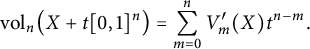 $$ \begin{align} \operatorname{\mathrm{vol}}_n\bigl(X + t[0,1]^n\bigr) = \sum_{m=0}^n V_m'(X) t^{n-m}. \end{align} $$
This formula implies in particular that the $\ell _1$
intrinsic volumes, like the Euclidean intrinsic volumes, are particular instances of mixed volumes [Reference Schneider33, Section 5.1]. Holmes–Thompson intrinsic volumes are not known to have representations as mixed volumes in general; furthermore, a Steiner-like formula such as (5.1), which would require the intrinsic volumes on the right-hand side to be mixed volumes of a particularly simple form, can only hold under additional restrictions on the normed space E. See [Reference Schneider32, Section 5] for some partial results and discussion of these issues.
$\ell _1$
intrinsic volumes, like the Euclidean intrinsic volumes, are particular instances of mixed volumes [Reference Schneider33, Section 5.1]. Holmes–Thompson intrinsic volumes are not known to have representations as mixed volumes in general; furthermore, a Steiner-like formula such as (5.1), which would require the intrinsic volumes on the right-hand side to be mixed volumes of a particularly simple form, can only hold under additional restrictions on the normed space E. See [Reference Schneider32, Section 5] for some partial results and discussion of these issues.
We end with a simple observation related to (5.1). As noted in [Reference Leinster and Meckes23], the quantity
 $$\begin{align*}\mathcal{W}'(X) = \sum_{m=0}^n V_m'(X) \end{align*}$$
is an $\ell _1$
analog of the Wills functional (see, e.g., [Reference Alonso-Gutiérrez, Hernández Cifre and Yepes Nicolás1]), which can be defined by
$\ell _1$
analog of the Wills functional (see, e.g., [Reference Alonso-Gutiérrez, Hernández Cifre and Yepes Nicolás1]), which can be defined by
 $$\begin{align*}\mathcal{W}(K) = \sum_{m=0}^n V_m(K). \end{align*}$$
The Wills functional was introduced in [Reference Wills42], where it was conjectured that
 $$\begin{align*}\# (K \cap \mathbb{Z}^n) \le \mathcal{W}(K) \end{align*}$$
for any $K \in \mathcal {K}^n$
. This was shown by Hadwiger [Reference Hadwiger14] to be false for sufficiently large n. However, (5.1) implies that an
$K \in \mathcal {K}^n$
. This was shown by Hadwiger [Reference Hadwiger14] to be false for sufficiently large n. However, (5.1) implies that an $\ell _1$
version of this conjecture is true in all dimensions.
$\ell _1$
version of this conjecture is true in all dimensions.
Proposition 5.1 Suppose that $X \subseteq \mathbb {R}^n$
is compact and
$X \subseteq \mathbb {R}^n$
is compact and $\ell _1$
-convex. Then
$\ell _1$
-convex. Then
 $$\begin{align*}\# (X \cap \mathbb{Z}^n) \le \mathcal{W}'(X). \end{align*}$$
Proof By (5.1),
 $$\begin{align*}\# (X \cap \mathbb{Z}^n) = \operatorname{\mathrm{vol}}_n\bigl((X\cap \mathbb{Z}^n) + [0,1]^n\bigr) \le \operatorname{\mathrm{vol}}_n\bigl(X + [0,1]^n\bigr) = \mathcal{W}'(X).\\[-35pt] \end{align*}$$
Acknowledgment
The author thanks the Mathematical Institute of the University of Oxford and Prof. Jon Keating for their hospitality, Thomas Wannerer for helpful comments and pointers to the literature on Holmes–Thompson intrinsic volumes, and an anonymous referee for helpful comments on the exposition.


 Open access