






















1. Introduction and main results
1.1 The setup
Let $\mathbf \Omega$
be a probability space and let
$\mathbf \Omega$
be a probability space and let $A_1, \ldots , A_n \subset {\mathbf \Omega }$
be events. We want to compute (or approximate)
$A_1, \ldots , A_n \subset {\mathbf \Omega }$
be events. We want to compute (or approximate)
 \begin{equation} {\mathbb P}\left ( \bigcap _{i=1}^n \overline {A}_i \right )=1- {\mathbb P}\left ( \bigcup _{i=1}^n A_i\right )\!, \end{equation}
the probability of the intersection of their complements. This is of course a fairly general problem, with many applications. In the usual interpretation, $A_i$
are some ‘bad’ events and so we are interested in the probability that none of them occurs. If the events
$A_i$
are some ‘bad’ events and so we are interested in the probability that none of them occurs. If the events $A_1, \ldots , A_n$
are independent, then
$A_1, \ldots , A_n$
are independent, then
 \begin{equation} {\mathbb P}\left ( \bigcap _{i=1}^n \overline {A}_i\right ) = \prod _{i=1}^n \left (1 - {\mathbb P}(A_i)\right )\!, \end{equation}
so to compute the left-hand side of (1.2) exactly, we only need to know the probabilities ${\mathbb P}(A_i)$
themselves.
${\mathbb P}(A_i)$
themselves.
We show that if the dependencies are controlled and the probabilities ${\mathbb P}(A_i)$
are sufficiently small, then the value of (1.1) can be efficiently approximated within an arbitrarily small relative error
${\mathbb P}(A_i)$
are sufficiently small, then the value of (1.1) can be efficiently approximated within an arbitrarily small relative error $0 \lt \epsilon \lt 1$
from the probabilities
$0 \lt \epsilon \lt 1$
from the probabilities
 \begin{equation*}{\mathbb P}( A_{i_1} \cap \ldots \cap A_{i_k}) \quad \text{where} \quad k = O ( \ln (n/\epsilon ))\end{equation*}
of the intersections of logarithmically many events $A_i$
.
$A_i$
.
Let $\Omega _1, \ldots , \Omega _m$
be probability spaces and let
$\Omega _1, \ldots , \Omega _m$
be probability spaces and let ${\mathbf \Omega } = \Omega _1 \times \cdots \times \Omega _m$
be their product. We write a point
${\mathbf \Omega } = \Omega _1 \times \cdots \times \Omega _m$
be their product. We write a point $x \in {\mathbf \Omega }$
as
$x \in {\mathbf \Omega }$
as $x=\left (\xi _1, \ldots , \xi _m\right )$
, where
$x=\left (\xi _1, \ldots , \xi _m\right )$
, where $\xi _j \in \Omega _j$
, and call
$\xi _j \in \Omega _j$
, and call $\xi _j$
coordinates of
$\xi _j$
coordinates of $x$
. We consider complex-valued random variables
$x$
. We consider complex-valued random variables $f\,:\, {\mathbf \Omega } \longrightarrow {\mathbb C}$
. For such an
$f\,:\, {\mathbf \Omega } \longrightarrow {\mathbb C}$
. For such an $f$
, we define the set of coordinates that
$f$
, we define the set of coordinates that $f$
depends on, as a subset
$f$
depends on, as a subset $\{\xi _j\,:\ j \in J_f \}$
where
$\{\xi _j\,:\ j \in J_f \}$
where $J_f \subset \{1, \ldots , m\}$
, such that for any two
$J_f \subset \{1, \ldots , m\}$
, such that for any two $x', x'' \in {\mathbf \Omega }$
, where
$x', x'' \in {\mathbf \Omega }$
, where $x'=\left (\xi _1', \ldots , \xi _m'\right )$
and
$x'=\left (\xi _1', \ldots , \xi _m'\right )$
and $x''=\left (\xi _1'', \ldots , \xi _m''\right )$
, we have
$x''=\left (\xi _1'', \ldots , \xi _m''\right )$
, we have $f(x')=f(x'')$
whenever
$f(x')=f(x'')$
whenever $\xi _j' = \xi ''_j$
for all
$\xi _j' = \xi ''_j$
for all $j \in J_f$
and there is no subset
$j \in J_f$
and there is no subset $J' \subsetneq J_f$
with that property. We say that
$J' \subsetneq J_f$
with that property. We say that $f$
depends on at most
$f$
depends on at most $r$
coordinates if
$r$
coordinates if $|J_f| \leq r$
. We say that two random variables
$|J_f| \leq r$
. We say that two random variables $f, g\,:\, {\mathbf \Omega } \longrightarrow {\mathbb C}$
share a coordinate if
$f, g\,:\, {\mathbf \Omega } \longrightarrow {\mathbb C}$
share a coordinate if $J_f \cap J_g \ne \emptyset$
, and any coordinate
$J_f \cap J_g \ne \emptyset$
, and any coordinate $\xi _j$
with
$\xi _j$
with $j \in J_f \cap J_g$
is called a shared coordinate of
$j \in J_f \cap J_g$
is called a shared coordinate of $f$
and
$f$
and $g$
.
$g$
.
Let $A \subset {\mathbf \Omega }$
be an event. The indicator of
$A \subset {\mathbf \Omega }$
be an event. The indicator of $A$
is the random variable
$A$
is the random variable $[A]\,:\, {\mathbf \Omega } \longrightarrow \{0, 1\}$
defined by
$[A]\,:\, {\mathbf \Omega } \longrightarrow \{0, 1\}$
defined by
 \begin{equation} [A](x)=\begin{cases} 1 &\text{if}\,\, x \in A \\ 0 & \text{if}\,\, x \notin A. \end{cases} \end{equation}
Similarly, we say that $A$
depends on at most
$A$
depends on at most $r$
coordinates if
$r$
coordinates if $[A]$
depends on at most
$[A]$
depends on at most $r$
coordinates, and that two events
$r$
coordinates, and that two events $A, B \subset {\mathbf \Omega }$
share a coordinate if
$A, B \subset {\mathbf \Omega }$
share a coordinate if $[A]$
and
$[A]$
and $[B]$
share a coordinate.
$[B]$
share a coordinate.
By $\overline {A}$
we denote the complement of an event
$\overline {A}$
we denote the complement of an event $A \subset {\mathbf \Omega }$
, so that
$A \subset {\mathbf \Omega }$
, so that $[\overline {A}]=1-[A]$
. We also note that
$[\overline {A}]=1-[A]$
. We also note that $[A] [B] = [A \cap B]$
for events
$[A] [B] = [A \cap B]$
for events $A, B \subset {\mathbf \Omega }$
.
$A, B \subset {\mathbf \Omega }$
.
We can now state the main result.
Theorem 1.
Let $\Omega _1, \ldots , \Omega _m$
be probability spaces and let
$\Omega _1, \ldots , \Omega _m$
be probability spaces and let ${\mathbf \Omega } = \Omega _1 \times \cdots \times \Omega _m$
be their product. Let
${\mathbf \Omega } = \Omega _1 \times \cdots \times \Omega _m$
be their product. Let $A_1, \ldots , A_n \subset {\mathbf \Omega }$
be events such that each event
$A_1, \ldots , A_n \subset {\mathbf \Omega }$
be events such that each event $A_i$
depends on at most
$A_i$
depends on at most $r_i$
coordinates and for each event
$r_i$
coordinates and for each event $A_i$
at most
$A_i$
at most $\Delta _i$
other events
$\Delta _i$
other events $A_j$
share a coordinate with
$A_j$
share a coordinate with $A_i$
. Let
$A_i$
. Let
 \begin{equation*}\Delta =\max \left \{5, \Delta _i\,:\, i=1, \ldots , n \right \}\end{equation*}
and let
 \begin{equation*}\mu _i=\min \{ r_i,\ \Delta _i+1\} \quad \text{for} \quad i=1, \ldots , n.\end{equation*}
Then for any $0 \lt \epsilon \lt 1$
there is
$0 \lt \epsilon \lt 1$
there is
 \begin{equation*}K=e^{O(\Delta )} \ln (n/\epsilon )\end{equation*}
such that whenever
 \begin{equation} {\mathbb P}(A_i) \ \lt \ (3 \Delta )^{-3\mu _i} \quad \text{for} \quad i=1, \ldots , n, \end{equation}
the value of ${\mathbb P}\left ( \bigcap _{i=1}^n \overline {A}_i \right )$
, up to relative error
${\mathbb P}\left ( \bigcap _{i=1}^n \overline {A}_i \right )$
, up to relative error $\epsilon$
, is determined by the probabilities of
$\epsilon$
, is determined by the probabilities of $k$
-wise intersections
$k$
-wise intersections
 \begin{equation} {\mathbb P} (A_{i_1} \cap \ldots \cap A_{i_k}), \quad \text{where} \quad k \leq K. \end{equation}
More precisely, for $1 \leq k \leq K$
, let
$1 \leq k \leq K$
, let
 \begin{equation} \sigma _k=\sum _{1 \leq i_1 \lt \ldots \lt i_k \leq n} {\mathbb P}(A_{i_1} \cap \ldots \cap A_{i_k} )\!. \end{equation}
Then for given $\Delta$
,
$\Delta$
, $n$
and
$n$
and $0\lt \epsilon \lt 1$
, there is a polynomial
$0\lt \epsilon \lt 1$
, there is a polynomial $Q=Q_{\Delta , n, \epsilon }$
in
$Q=Q_{\Delta , n, \epsilon }$
in $K$
variables and with deg
$K$
variables and with deg $Q \leq K$
, such that
$Q \leq K$
, such that
 \begin{equation*}\left | \ln {\mathbb P}\left ( \bigcap _{i=1}^n \overline {A}_i\right ) - Q\left (\sigma _1, \ldots , \sigma _K\right ) \right | \ \leq \ \epsilon ,\end{equation*}
provided ( 1.4 ) holds.
The implied constant in the ‘ $O$
’ notation is absolute.
$O$
’ notation is absolute.
Note that an additive $\epsilon$
-approximation of
$\epsilon$
-approximation of $\ln {\mathbb P}\left ( \bigcap _{i=1}^n \overline {A}_i\right )$
translates into a relative
$\ln {\mathbb P}\left ( \bigcap _{i=1}^n \overline {A}_i\right )$
translates into a relative $\epsilon$
-approximation of
$\epsilon$
-approximation of ${\mathbb P}\left ( \bigcap _{i=1}^n \overline {A}_i\right )$
. We are interested in the regime where
${\mathbb P}\left ( \bigcap _{i=1}^n \overline {A}_i\right )$
. We are interested in the regime where $r_i$
and
$r_i$
and $\Delta$
are small (fixed in advance), while
$\Delta$
are small (fixed in advance), while $n, m$
and
$n, m$
and $1/\epsilon$
are allowed to grow.
$1/\epsilon$
are allowed to grow.
The polynomial $Q$
has rational coefficients, and given
$Q$
has rational coefficients, and given $\sigma _1, \ldots , \sigma _K$
, its value
$\sigma _1, \ldots , \sigma _K$
, its value $Q(\sigma _1, \ldots , \sigma _K)$
can be computed efficiently, in polynomial in
$Q(\sigma _1, \ldots , \sigma _K)$
can be computed efficiently, in polynomial in $K$
time, so the main difficulty is in computing
$K$
time, so the main difficulty is in computing $\sigma _k$
. Computing probabilities (1.5) reduces to operating with
$\sigma _k$
. Computing probabilities (1.5) reduces to operating with $R=r_{i_1} + \ldots + r_{i_k}$
coordinates and often can be done roughly in exponential in
$R=r_{i_1} + \ldots + r_{i_k}$
coordinates and often can be done roughly in exponential in $R$
time, which leads to an approximation algorithm of a quasi-polynomial
$R$
time, which leads to an approximation algorithm of a quasi-polynomial $n^{O(\ln (n/\epsilon ))}$
complexity, if
$n^{O(\ln (n/\epsilon ))}$
complexity, if $\Delta$
and
$\Delta$
and $r_i$
are bounded above by constants, fixed in advance. Moreover, in some situations the combinatorial methods of [Reference Patel and Regts25] and [Reference Liu, Sinclair and Srivastava20] may sharpen it to a genuinely polynomial time algorithm (more on that is in Section 2.2 below).
$r_i$
are bounded above by constants, fixed in advance. Moreover, in some situations the combinatorial methods of [Reference Patel and Regts25] and [Reference Liu, Sinclair and Srivastava20] may sharpen it to a genuinely polynomial time algorithm (more on that is in Section 2.2 below).
We would like to argue that the form of the approximation for $\ln {\mathbb P}\left ( \bigcap _{i=1}^n \overline {A}_i\right )$
obtained in Theorem 1, that is, a polynomial in
$\ln {\mathbb P}\left ( \bigcap _{i=1}^n \overline {A}_i\right )$
obtained in Theorem 1, that is, a polynomial in $\sigma _k$
, should not look completely unexpected. When the events
$\sigma _k$
, should not look completely unexpected. When the events $A_1, \ldots , A_n$
are independent, from (1.2), we can write
$A_1, \ldots , A_n$
are independent, from (1.2), we can write
 \begin{equation*}\ln {\mathbb P}\left ( \bigcap _{i=1}^n \overline {A}_i\right )= \sum _{i=1}^n \ln (1-{\mathbb P}(A_i)).\end{equation*}
Assuming that ${\mathbb P}(A_i) \lt \alpha$
for some fixed
${\mathbb P}(A_i) \lt \alpha$
for some fixed $\alpha \lt 1$
, we can approximate the logarithms by their Taylor polynomials:
$\alpha \lt 1$
, we can approximate the logarithms by their Taylor polynomials:
 \begin{equation*}\ln ( 1- {\mathbb P}(A_i)) \approx -\sum _{k=1}^K \frac {1}{k} ({\mathbb P}(A_i))^k \quad \text{and} \quad \ln {\mathbb P}\left ( \bigcap _{i=1}^n \overline {A}_i\right ) \approx - \sum _{k=1}^K \frac {1}{k} \left ( \sum _{i=1}^n ({\mathbb P}(A_i))^k\right ). \end{equation*}
The Newton identities allow us to write the inner sums $\sum _{i=1}^n ({\mathbb P}(A_i))^k$
as polynomials in elementary symmetric functions
$\sum _{i=1}^n ({\mathbb P}(A_i))^k$
as polynomials in elementary symmetric functions
 \begin{equation*}\sum _{1 \leq i_1 \lt \ldots \lt i_k \leq n} {\mathbb P}(A_{i_1}) \cdots {\mathbb P}(A_{i_k})\end{equation*}
and hence as polynomials in $\sigma _k$
, as we have in Theorem 1.
$\sigma _k$
, as we have in Theorem 1.
We note that one can always assume that $r_i \leq 2^{\Delta _i}$
(we will not use it). Indeed, let us choose an event, without loss of generality,
$r_i \leq 2^{\Delta _i}$
(we will not use it). Indeed, let us choose an event, without loss of generality, $A_n$
. Let
$A_n$
. Let $I \subset \{1, \ldots , n-1\}$
be the set of indices
$I \subset \{1, \ldots , n-1\}$
be the set of indices $i$
such that
$i$
such that $A_i$
shares a coordinate with
$A_i$
shares a coordinate with $A_n$
, so that
$A_n$
, so that $|I| \leq \Delta _n$
. Let
$|I| \leq \Delta _n$
. Let $J \subset \{1, \ldots , m\}$
be the set of indices
$J \subset \{1, \ldots , m\}$
be the set of indices $j$
such that
$j$
such that $A_n$
depends on the coordinate
$A_n$
depends on the coordinate $\xi _j$
, so that
$\xi _j$
, so that $|J| \leq r_n$
. With each
$|J| \leq r_n$
. With each $j \in J$
we associate a subset
$j \in J$
we associate a subset $I_j \subset I$
consisting of all indices
$I_j \subset I$
consisting of all indices $i \in I$
such that
$i \in I$
such that $A_i$
depends on
$A_i$
depends on $\xi _j$
. Now, all coordinates
$\xi _j$
. Now, all coordinates $\xi _j$
with the same associated subset
$\xi _j$
with the same associated subset $I_j$
can be ‘lumped together’ into a single coordinate. For example, if
$I_j$
can be ‘lumped together’ into a single coordinate. For example, if $A_n$
does not share a coordinate with any other event
$A_n$
does not share a coordinate with any other event $A_i$
, then all the coordinates that
$A_i$
, then all the coordinates that $A_n$
depends on can be considered as a single coordinate in the probability product space, and if
$A_n$
depends on can be considered as a single coordinate in the probability product space, and if $A_n$
shares a coordinate with exactly one other event, say
$A_n$
shares a coordinate with exactly one other event, say $A_1$
, then all the coordinates shared by
$A_1$
, then all the coordinates shared by $A_n$
and
$A_n$
and $A_1$
can be considered as a single coordinate in the product space, while all remaining coordinates, if any, that
$A_1$
can be considered as a single coordinate in the product space, while all remaining coordinates, if any, that $A_n$
depends on can be considered as another coordinate. Since there are
$A_n$
depends on can be considered as another coordinate. Since there are $2^{|I|} \leq 2^{\Delta _n}$
subsets of
$2^{|I|} \leq 2^{\Delta _n}$
subsets of $I$
, in the end we obtain at most
$I$
, in the end we obtain at most $2^{\Delta _n}$
coordinates for
$2^{\Delta _n}$
coordinates for $A_n$
.
$A_n$
.
The bound (1.4) is unlikely to be optimal, though some upper bound in terms of $\Delta$
is definitely needed, since otherwise even deciding whether
$\Delta$
is definitely needed, since otherwise even deciding whether ${\mathbb P}\left (\bigcap _{i=1}^n \overline {A}_i\right ) \gt 0$
can be quite hard. It would be interesting to find out whether there has to be an exponential dependence on
${\mathbb P}\left (\bigcap _{i=1}^n \overline {A}_i\right ) \gt 0$
can be quite hard. It would be interesting to find out whether there has to be an exponential dependence on $\mu _i$
.
$\mu _i$
.
We now give a simple example of how Theorem 1 can be applied.
1.2 Example: Counting integer points
Let $\ell _1, \ldots , \ell _n\,:\, {\mathbb R}^m \longrightarrow {\mathbb R}$
be polynomials. In the cube
$\ell _1, \ldots , \ell _n\,:\, {\mathbb R}^m \longrightarrow {\mathbb R}$
be polynomials. In the cube $C=[0, c]^m \subset {\mathbb R}^m$
, where
$C=[0, c]^m \subset {\mathbb R}^m$
, where $c$
is a positive integer, we consider the set
$c$
is a positive integer, we consider the set
 \begin{equation} S =\bigl \{ x \in C \cap {\mathbb Z^m}\,: \quad \ell _i(x) \ \leq \ 0 \quad \text{for} \quad i=1, \ldots , n \bigr \} \end{equation}
of integer points, satisfying a system of polynomial inequalities.
Suppose further that each polynomial $\ell _i$
depends on at most
$\ell _i$
depends on at most $r$
coordinates of
$r$
coordinates of $x \in {\mathbb R}^m$
,
$x \in {\mathbb R}^m$
, $x=\left (\xi _1, \ldots , \xi _m\right )$
, and that for each polynomial
$x=\left (\xi _1, \ldots , \xi _m\right )$
, and that for each polynomial $\ell _i$
there are not more than
$\ell _i$
there are not more than $\Delta$
of other polynomials
$\Delta$
of other polynomials $\ell _j$
that depend on some of the same coordinates. We assume that
$\ell _j$
that depend on some of the same coordinates. We assume that $r$
and
$r$
and $\Delta$
are fixed in advance, while
$\Delta$
are fixed in advance, while $n$
,
$n$
, $m$
, and
$m$
, and $c$
can vary. We want to approximate the cardinality
$c$
can vary. We want to approximate the cardinality $|S|$
of
$|S|$
of $S$
.
$S$
.
For $i=1, \ldots , m$
, we interpret the set
$i=1, \ldots , m$
, we interpret the set ${\mathbb Z} \cap [0, c]$
of integer points in an interval as a probability space
${\mathbb Z} \cap [0, c]$
of integer points in an interval as a probability space $\Omega _i$
with the uniform measure, and let
$\Omega _i$
with the uniform measure, and let ${\mathbf \Omega }= \Omega _1 \times \cdots \times \Omega _m$
. We further introduce events
${\mathbf \Omega }= \Omega _1 \times \cdots \times \Omega _m$
. We further introduce events
 \begin{equation*}A_i=\bigl \{x \in C \cap {\mathbb Z}^m\,: \quad \ell _i(x) \gt 0 \bigr \} \quad \text{for} \quad i=1, \ldots , n\end{equation*}
and see that
 \begin{equation*}|S| =(c+1)^m {\mathbb P}\left ( \bigcap _{i=1}^n \overline {A}_i\right ).\end{equation*}
Suppose now that
 \begin{equation*}{\mathbb P}(A_i)= |A_i| (c+1)^{-m} \ \lt \ (3 \Delta )^{-3r} \quad \text{for} \quad i=1, \ldots , n.\end{equation*}
Theorem 1 then asserts that up to a relative error $0 \lt \epsilon \lt 1$
, the cardinality of
$0 \lt \epsilon \lt 1$
, the cardinality of $S$
is determined by the cardinalities
$S$
is determined by the cardinalities
 \begin{equation} A_{i_1} \cap \ldots \cap A_{i_k} = \bigl \{x \in C\cap {\mathbb Z}^m\,: \quad \ell _{i_1}(x) \gt 0, \ldots , \ell _{i_k}(x) \gt 0 \bigr \} \end{equation}
for $k=O\left (\ln (n/\epsilon )\right )$
. We note that the inequalities in (1.8) involve at most
$k=O\left (\ln (n/\epsilon )\right )$
. We note that the inequalities in (1.8) involve at most $k r$
coordinates
$k r$
coordinates $\xi _j$
, so that we can compute the probability of each intersection (1.8) in the most straightforward way by enumerating
$\xi _j$
, so that we can compute the probability of each intersection (1.8) in the most straightforward way by enumerating $(c+1)^{rk}$
integer points, which in the end results in an approximation algorithm to count points in (1.7) of
$(c+1)^{rk}$
integer points, which in the end results in an approximation algorithm to count points in (1.7) of $\left (m(c+1)\right )^{O\left ( \ln (n/\epsilon )\right )}$
complexity.
$\left (m(c+1)\right )^{O\left ( \ln (n/\epsilon )\right )}$
complexity.
If $\deg \ell _i \leq 1$
for
$\deg \ell _i \leq 1$
for $i=1, \ldots , n$
, we can do better: in this case,
$i=1, \ldots , n$
, we can do better: in this case, $A_i$
is the set of integer points in a semi-open polyhedron, and the exact enumeration in (1.8) can be done with
$A_i$
is the set of integer points in a semi-open polyhedron, and the exact enumeration in (1.8) can be done with
 \begin{equation*} ((1 + \ln c)(kr) )^{O (kr \ln (kr) )}\end{equation*}
complexity, see [Reference Barvinok1], which leads to a quasi-polynomial algorithm for approximating the number of integer points in (1.7).
Similar algorithms can be designed for computing volumes, in which case the probability spaces $\Omega _i$
are identified with intervals and hence become infinite, see also [Reference Gritzmann and Klee10] for the complexity of (deterministic) volume computation in small dimensions.
$\Omega _i$
are identified with intervals and hence become infinite, see also [Reference Gritzmann and Klee10] for the complexity of (deterministic) volume computation in small dimensions.
1.3 Connections
The Lovász Local Lemma [Reference Erdős and Lovász8] provides a sufficient criterion for the event $\bigcap _{i=1}^n \overline {A}_i$
to have positive probability. Namely, for each
$\bigcap _{i=1}^n \overline {A}_i$
to have positive probability. Namely, for each $i=1, \ldots , n$
, let
$i=1, \ldots , n$
, let $\Gamma _i \subset \{1, \ldots , n\}$
be the set of indices
$\Gamma _i \subset \{1, \ldots , n\}$
be the set of indices $j \ne i$
such that
$j \ne i$
such that $A_j$
shares a coordinate with
$A_j$
shares a coordinate with $A_i$
. Suppose that there are numbers
$A_i$
. Suppose that there are numbers $0 \lt s_i \lt 1$
for
$0 \lt s_i \lt 1$
for $i=1, \ldots , n$
, such that
$i=1, \ldots , n$
, such that
 \begin{equation} {\mathbb P}(A_i) \ \leq \ s_i \prod _{j \in \Gamma _i} (1-s_j) \quad \text{for} \quad i=1, \ldots , n. \end{equation}
Then
 \begin{equation} {\mathbb P}\left (\bigcap _{i=1}^n \overline {A}_i \right ) \ \geq \ \prod _{j=1}^n (1-s_i) \ \gt \ 0. \end{equation}
As in Theorem 1, let $\Delta$
be an upper bound on the number of events
$\Delta$
be an upper bound on the number of events $A_j$
that share a coordinate with any particular event
$A_j$
that share a coordinate with any particular event $A_i$
. Let us choose
$A_i$
. Let us choose $s_i=\frac {1}{\Delta }$
for
$s_i=\frac {1}{\Delta }$
for $i=1, \ldots , n$
in (1.9). Then for the right-hand side of (1.9), we have
$i=1, \ldots , n$
in (1.9). Then for the right-hand side of (1.9), we have
 \begin{equation*} s_i \prod _{j \in \Gamma _i} (1-s_j) \ \geq \ \frac {1}{\Delta } \left (1 - \frac {1}{\Delta }\right )^{\Delta } \sim \frac {1}{e \Delta }, \end{equation*}
and hence our condition (1.4) is much more restrictive than (1.9). The constraints (1.9) and the lower bound (1.10) are, in fact, sharp [Reference Shearer28] for the intersection $\bigcap _{i=1}^n \overline {A}_i$
to have positive probability, see also [Reference Scott and Sokal27] and [Reference Jenssen, Fischer and Johnson14]. We, however, are interested in further approximating that probability arbitrarily closely.
$\bigcap _{i=1}^n \overline {A}_i$
to have positive probability, see also [Reference Scott and Sokal27] and [Reference Jenssen, Fischer and Johnson14]. We, however, are interested in further approximating that probability arbitrarily closely.
There has been a lot of work on how to approximate ${\mathbb P}\left (\bigcap _{i=1}^n \overline {A}_i\right )$
under some conditions, similar to (1.9). This includes randomised algorithms, see [Reference Jerrum15] for a survey of the partial rejection sampling approach inspired by the algorithmic proof [Reference Moser and Tardos24] of the Lovász Local Lemma, as well as deterministic, see [Reference Moitra23, Reference Jain, Pham and Vuong13, Reference He, Wang and Yin12, Reference Wang and Yin29] and references therein. It appears that they all operate under some additional assumptions, either restricting the intersection pattern of
${\mathbb P}\left (\bigcap _{i=1}^n \overline {A}_i\right )$
under some conditions, similar to (1.9). This includes randomised algorithms, see [Reference Jerrum15] for a survey of the partial rejection sampling approach inspired by the algorithmic proof [Reference Moser and Tardos24] of the Lovász Local Lemma, as well as deterministic, see [Reference Moitra23, Reference Jain, Pham and Vuong13, Reference He, Wang and Yin12, Reference Wang and Yin29] and references therein. It appears that they all operate under some additional assumptions, either restricting the intersection pattern of $A_i$
to ‘extremal’ where
$A_i$
to ‘extremal’ where $A_i \cap A_j =\emptyset$
whenever
$A_i \cap A_j =\emptyset$
whenever $A_i$
and
$A_i$
and $A_j$
share a coordinate [Reference Jerrum15], or restricting the structure of the sets
$A_j$
share a coordinate [Reference Jerrum15], or restricting the structure of the sets $A_i$
, such as to those coming from CNF Boolean formulas [Reference Moitra23] or atomic clauses with one violation per clause [Reference Wang and Yin29], or assuming that each
$A_i$
, such as to those coming from CNF Boolean formulas [Reference Moitra23] or atomic clauses with one violation per clause [Reference Wang and Yin29], or assuming that each $\Omega _i$
is a finite set with uniform measure and an upper bound on the number of elements in
$\Omega _i$
is a finite set with uniform measure and an upper bound on the number of elements in $\Omega _i$
[Reference Jain, Pham and Vuong13, Reference He, Wang and Yin12].
$\Omega _i$
[Reference Jain, Pham and Vuong13, Reference He, Wang and Yin12].
Thus Theorem 1 establishes a new regime, where approximate counting of satisfying assignments in the constraint satisfaction problem can be done efficiently, in quasi-polynomial time. For each formula, we need to bound from above the probability that it is not satisfied and also bound the degree of the dependency graph of the formulas, but we do not need to assume anything about the combinatorics of the set $A_i$
of assignments where a particular formula is not satisfied, see also Section 4.2.
$A_i$
of assignments where a particular formula is not satisfied, see also Section 4.2.
Bencs and Regts [Reference Bencs and G. Regts6] and then Guo and N [Reference Guo and Vishvajeet11] used an approach somewhat similar to ours to approximate volumes of some combinatorially defined polytopes in deterministic polynomial time (we talk more about the similarities and differences of the approaches in Section 2.2 and Section 4.1). After the first version of this paper appeared as a preprint, Mann and Waite [Reference Mann and Waite22] discussed approximating (1.1), among other questions. They applied the method of cluster expansion, which we discuss in Section 4.1.
Linial and Nisan [Reference Linial and Nisan19] and then Kahn, Linial, and Samorodnitsky [Reference Kahn, Linial and Samorodnitsky16] considered the problem of approximating ${\mathbb P} \left (\bigcup _{i=1}^n A_i \right )$
from the probabilities
${\mathbb P} \left (\bigcup _{i=1}^n A_i \right )$
from the probabilities ${\mathbb P} (A_{i_1} \cap \ldots \cap A_{i_k})$
of
${\mathbb P} (A_{i_1} \cap \ldots \cap A_{i_k})$
of $k$
-wise intersections, without assuming anything about the dependencies of
$k$
-wise intersections, without assuming anything about the dependencies of $A_i$
. In [Reference Linial and Nisan19], Linial and Nisan showed in particular that for
$A_i$
. In [Reference Linial and Nisan19], Linial and Nisan showed in particular that for $k = \Omega (\sqrt {n})$
, the probability of the union can be approximated from the probabilities of
$k = \Omega (\sqrt {n})$
, the probability of the union can be approximated from the probabilities of $k$
-wise intersections within a relative error of
$k$
-wise intersections within a relative error of $O\left (e^{-2k/\sqrt {n}}\right )$
and that for
$O\left (e^{-2k/\sqrt {n}}\right )$
and that for $k=O(\sqrt {n})$
the probability of the union cannot be approximated better than within a factor of
$k=O(\sqrt {n})$
the probability of the union cannot be approximated better than within a factor of $O(n/k^2)$
. Then in [Reference Kahn, Linial and Samorodnitsky16], Kahn, Linial, and Samorodnitsky proved that for any
$O(n/k^2)$
. Then in [Reference Kahn, Linial and Samorodnitsky16], Kahn, Linial, and Samorodnitsky proved that for any $k$
, the probability of the union can be approximated from the probability of the
$k$
, the probability of the union can be approximated from the probability of the $k$
-wise intersections within an additive error of
$k$
-wise intersections within an additive error of $e^{-\Omega \left (\frac {k^2}{n \ln n}\right )}$
and that the result is sharp, up to a logarithmic factor in the exponent. Since in our case
$e^{-\Omega \left (\frac {k^2}{n \ln n}\right )}$
and that the result is sharp, up to a logarithmic factor in the exponent. Since in our case ${\mathbb P}\left ( \bigcap _{i=1}^n \overline {A}_i\right )$
can be exponentially small in
${\mathbb P}\left ( \bigcap _{i=1}^n \overline {A}_i\right )$
can be exponentially small in $n$
, an attempt to combine the estimates of [Reference Linial and Nisan19] and [Reference Kahn, Linial and Samorodnitsky16] and the obvious formula (1.1) can produce a huge relative error in estimating the probability of the intersection.
$n$
, an attempt to combine the estimates of [Reference Linial and Nisan19] and [Reference Kahn, Linial and Samorodnitsky16] and the obvious formula (1.1) can produce a huge relative error in estimating the probability of the intersection.
The methods of [Reference Linial and Nisan19] and [Reference Kahn, Linial and Samorodnitsky16] on the one hand, and the method of this paper on the other hand, seem to be quite different. In particular, the final answer is given in different forms: in [Reference Linial and Nisan19] and [Reference Kahn, Linial and Samorodnitsky16], the value of ${\mathbb P}\left ( \bigcup _{i=1}^n A_i\right )$
is approximated by a linear function in the quantities
${\mathbb P}\left ( \bigcup _{i=1}^n A_i\right )$
is approximated by a linear function in the quantities $\sigma _k$
of (1.6), whereas our Theorem 1 approximates
$\sigma _k$
of (1.6), whereas our Theorem 1 approximates $\ln {\mathbb P} \left ( \bigcap _{i=1}^n \overline {A}_i\right )$
by a polynomial in
$\ln {\mathbb P} \left ( \bigcap _{i=1}^n \overline {A}_i\right )$
by a polynomial in $\sigma _k$
. Nevertheless, it feels like the approaches must be somehow related. In particular, the wording of one of the results of [Reference Kahn, Linial and Samorodnitsky16] comes tantalisingly close to the wording of our Theorem 1: it is proved in [Reference Kahn, Linial and Samorodnitsky16] that the number, say
$\sigma _k$
. Nevertheless, it feels like the approaches must be somehow related. In particular, the wording of one of the results of [Reference Kahn, Linial and Samorodnitsky16] comes tantalisingly close to the wording of our Theorem 1: it is proved in [Reference Kahn, Linial and Samorodnitsky16] that the number, say $s$
, of satisfying assignments of a Boolean DNF formula in
$s$
, of satisfying assignments of a Boolean DNF formula in $n$
variables is determined exactly by the set of numbers of satisfying assignments for all conjunctions of
$n$
variables is determined exactly by the set of numbers of satisfying assignments for all conjunctions of $k \leq \log _2 n +1$
terms of the formula, although it is not clear how to compute that
$k \leq \log _2 n +1$
terms of the formula, although it is not clear how to compute that $s$
from that set of numbers.
$s$
from that set of numbers.
2. The method of the proof of Theorem 1 and preliminaries
2.1 The method
Let $\mathbf \Omega$
be the probability space and let
$\mathbf \Omega$
be the probability space and let $A_1, \ldots , A_n \subset {\mathbf \Omega }$
be events as in Theorem 1. We define a univariate polynomial of a complex variable
$A_1, \ldots , A_n \subset {\mathbf \Omega }$
be events as in Theorem 1. We define a univariate polynomial of a complex variable $z$
by
$z$
by
 \begin{equation} p(z)=\int _{{\mathbf \Omega }} \prod _{i=1}^n (1-z [A_i]) \ dx, \end{equation}
where $[A_i]$
is the indicator of
$[A_i]$
is the indicator of $A_i$
defined by (1.3) and
$A_i$
defined by (1.3) and $dx$
stands for the integration against the product probability measure in
$dx$
stands for the integration against the product probability measure in $\mathbf \Omega$
. Then
$\mathbf \Omega$
. Then
 \begin{equation*}p(1)=\int _{{\mathbf \Omega }} \prod _{i=1}^n (1-[A_i]) \ dx = {\mathbb P}\left ( \bigcap _{i=1}^n \overline {A}_i \right )\!.\end{equation*}
On the other hand, $p(0)=1$
and for the
$p(0)=1$
and for the $k$
-th derivative of
$k$
-th derivative of $p$
at
$p$
at $0$
we have
$0$
we have
 \begin{equation} \begin{aligned} p^{(k)}(0)=&(\!-\!1)^k k! \sum _{1 \leq i_1 \lt i_2 \lt \ldots \lt i_k \leq n} \int _{{\mathbf \Omega }} [A_{i_1}] \cdots [A_{i_k}] \ dx \\= &(\!-\!1)^k k! \sum _{1 \leq i_1 \lt i_2 \lt \ldots \lt i_k \leq n} {\mathbb P}\left (A_{i_1} \cap \ldots \cap A_{i_k}\right ) \\= &(\!-\!1)^k k! \sigma _k. \end{aligned} \end{equation}
Clearly, $\deg p \leq n$
. Thus our goal is to approximate
$\deg p \leq n$
. Thus our goal is to approximate $p(1)$
within relative error
$p(1)$
within relative error $\epsilon$
from
$\epsilon$
from $p^{(k)}(0)$
with
$p^{(k)}(0)$
with $k =O(\ln (n/\epsilon ))$
.
$k =O(\ln (n/\epsilon ))$
.
2.2
Approximating $p(1)$
from
$p^{(k)}(0)$
$p(1)$
from
$p^{(k)}(0)$


It turns out that for our purposes it suffices to show that $p(z) \ne 0$
in some neighbourhood of the interval
$p(z) \ne 0$
in some neighbourhood of the interval $[0, 1]$
in the complex plane
$[0, 1]$
in the complex plane $\mathbb C$
. More precisely, if a polynomial
$\mathbb C$
. More precisely, if a polynomial $g(z)$
with
$g(z)$
with $\deg g \leq n$
does not have zeros in a
$\deg g \leq n$
does not have zeros in a $\delta$
-neighbourhood of
$\delta$
-neighbourhood of $[0, 1] \subset {\mathbb C}$
for some
$[0, 1] \subset {\mathbb C}$
for some $0 \lt \delta \lt 1$
, then for any
$0 \lt \delta \lt 1$
, then for any $0 \lt \epsilon \lt 1$
, the value of
$0 \lt \epsilon \lt 1$
, the value of $g(1)$
, up to relative error
$g(1)$
, up to relative error $\epsilon$
(properly defined if
$\epsilon$
(properly defined if $g(1)$
is a non-zero complex number), is determined by
$g(1)$
is a non-zero complex number), is determined by $g^{(k)}(0)$
for
$g^{(k)}(0)$
for $k \leq K=e^{O(1/\delta )}\ln (n/\epsilon )$
. Given the values
$k \leq K=e^{O(1/\delta )}\ln (n/\epsilon )$
. Given the values $g(0), g'(0), \ldots , g^{(K)}(0)$
, the approximation can be computed in
$g(0), g'(0), \ldots , g^{(K)}(0)$
, the approximation can be computed in $O(K^3)$
time. Furthermore, if
$O(K^3)$
time. Furthermore, if $g(0)=1$
then an approximation of
$g(0)=1$
then an approximation of $\ln g(1)$
within additive error
$\ln g(1)$
within additive error $\epsilon$
can be written as a polynomial
$\epsilon$
can be written as a polynomial $Q$
in
$Q$
in $g^{(k)}(0)$
with
$g^{(k)}(0)$
with $k \leq K$
and
$k \leq K$
and $\deg Q \leq K$
. Below we briefly describe how it is done, see Section 2.2 of [Reference Barvinok2] and also [Reference Barvinok3] for detail.
$\deg Q \leq K$
. Below we briefly describe how it is done, see Section 2.2 of [Reference Barvinok2] and also [Reference Barvinok3] for detail.
Suppose we have a univariate polynomial $g\,:\, {\mathbb C} \longrightarrow {\mathbb C}$
of degree
$g\,:\, {\mathbb C} \longrightarrow {\mathbb C}$
of degree $n \geq 1$
such that
$n \geq 1$
such that $g(z) \ne 0$
in the disc
$g(z) \ne 0$
in the disc $|z| \lt \beta$
of some radius
$|z| \lt \beta$
of some radius $\beta \gt 1$
. We can choose a branch of
$\beta \gt 1$
. We can choose a branch of $f(z)=\ln g(z)$
in the disc and consider the Taylor polynomial of
$f(z)=\ln g(z)$
in the disc and consider the Taylor polynomial of $T_m(z)$
of degree
$T_m(z)$
of degree $m \geq 1$
of
$m \geq 1$
of $f(z)$
, computed at
$f(z)$
, computed at $z=0$
:
$z=0$
:
 \begin{equation*}T_m(z)=f(0)+\sum _{k=1}^m \frac {f^{(k)}(0)}{k!} z^k.\end{equation*}
It turns out that $T_m(1)$
approximates
$T_m(1)$
approximates $f(1)$
within an additive error that decreases exponentially with
$f(1)$
within an additive error that decreases exponentially with $m$
:
$m$
:
 \begin{equation*}\left | f(z) - T_m(z)\right | \ \leq \ \frac {n}{(m+1) \beta ^m (\beta -1)} \quad \text{provided} \quad |z| \leq 1.\end{equation*}
Hence to approximate $f(1)$
by
$f(1)$
by $T_m(1)$
, respectively
$T_m(1)$
, respectively $g(1)$
by
$g(1)$
by $\exp \left \{T_m(1)\right \}$
, within an additive error, respectively relative error, of
$\exp \left \{T_m(1)\right \}$
, within an additive error, respectively relative error, of $0 \lt \epsilon \lt 1$
, one can choose
$0 \lt \epsilon \lt 1$
, one can choose $m=O_{\beta }\left (\ln (n/\epsilon )\right )$
. Moreover, the derivatives
$m=O_{\beta }\left (\ln (n/\epsilon )\right )$
. Moreover, the derivatives $f^{(k)}(0)$
for
$f^{(k)}(0)$
for $k=1, \ldots , m$
are computed from the derivatives
$k=1, \ldots , m$
are computed from the derivatives $g^{(k)}(0)$
for
$g^{(k)}(0)$
for $k=1, \ldots , m$
by solving an
$k=1, \ldots , m$
by solving an $m \times m$
system of linear equations with an invertible triangular matrix having
$m \times m$
system of linear equations with an invertible triangular matrix having $g(0) \ne 0$
on the diagonal.
$g(0) \ne 0$
on the diagonal.
Suppose now the polynomial $g$
satisfies a weaker condition or being non-zero in a
$g$
satisfies a weaker condition or being non-zero in a $\delta$
-neighbourhood
$\delta$
-neighbourhood $U$
of the interval
$U$
of the interval $[0, 1] \subset {\mathbb C}$
. Then one can reduce it to the already considered case of a polynomial that is non-zero in a disc, by replacing
$[0, 1] \subset {\mathbb C}$
. Then one can reduce it to the already considered case of a polynomial that is non-zero in a disc, by replacing $g(z)$
with the composition
$g(z)$
with the composition $h(z)=g(\phi (z))$
, where
$h(z)=g(\phi (z))$
, where $\phi \,:\, {\mathbb C} \longrightarrow {\mathbb C}$
is an explicit polynomial such that
$\phi \,:\, {\mathbb C} \longrightarrow {\mathbb C}$
is an explicit polynomial such that $\phi (0)=0$
,
$\phi (0)=0$
, $\phi (1)=1$
, and
$\phi (1)=1$
, and $\phi$
maps the disc
$\phi$
maps the disc $\{z\,:\, |z| \leq \beta \}$
with some
$\{z\,:\, |z| \leq \beta \}$
with some $\beta =1+ e^{-O(1/\delta )}$
inside
$\beta =1+ e^{-O(1/\delta )}$
inside $U$
. We have
$U$
. We have $\deg h=\deg g + \deg \phi$
and since
$\deg h=\deg g + \deg \phi$
and since $\phi (0)=0$
, the derivatives
$\phi (0)=0$
, the derivatives $h^{(k)}(0)$
for
$h^{(k)}(0)$
for $k=1, \ldots , m$
are computed from the derivatives
$k=1, \ldots , m$
are computed from the derivatives $g^{(k)}(0)$
for
$g^{(k)}(0)$
for $k=1, \ldots , m$
.
$k=1, \ldots , m$
.
We show that for some $\delta =O(1/\Delta )$
and
$\delta =O(1/\Delta )$
and $p(z)$
defined by (2.1), we indeed have
$p(z)$
defined by (2.1), we indeed have $p(z) \ne 0$
in the
$p(z) \ne 0$
in the $\delta$
-neighbourhood of
$\delta$
-neighbourhood of $[0, 1] \subset {\mathbb C}$
, assuming the hypothesis of Theorem 1. Assuming that the values of
$[0, 1] \subset {\mathbb C}$
, assuming the hypothesis of Theorem 1. Assuming that the values of $\sigma _k$
defined by (1.6) can be computed in
$\sigma _k$
defined by (1.6) can be computed in $n^{O(k)}$
time, the straightforward approach of [Reference Barvinok2] and [Reference Barvinok3] allows one to approximate
$n^{O(k)}$
time, the straightforward approach of [Reference Barvinok2] and [Reference Barvinok3] allows one to approximate $p(1)={\mathbb P}\left ( \bigcap _{i=1}^n \overline {A}_i\right )$
within relative error
$p(1)={\mathbb P}\left ( \bigcap _{i=1}^n \overline {A}_i\right )$
within relative error $\epsilon$
in quasi-polynomial
$\epsilon$
in quasi-polynomial $n^{O\left ( \ln (n/\epsilon )\right )}$
time, provided we consider
$n^{O\left ( \ln (n/\epsilon )\right )}$
time, provided we consider $\Delta$
to be fixed in advance.
$\Delta$
to be fixed in advance.
If we assume that ${\mathbb P}\left (A_{i_1}\cap \ldots \cap A_{i_k}\right )$
can be computed in
${\mathbb P}\left (A_{i_1}\cap \ldots \cap A_{i_k}\right )$
can be computed in $2^{O(k)}$
time, there is a possibility of a speed-up to a genuinely polynomial time, using the approach of Patel and Regts [Reference Patel and Regts25], see also [Reference Liu, Sinclair and Srivastava20]. Here, we very briefly sketch how. With events
$2^{O(k)}$
time, there is a possibility of a speed-up to a genuinely polynomial time, using the approach of Patel and Regts [Reference Patel and Regts25], see also [Reference Liu, Sinclair and Srivastava20]. Here, we very briefly sketch how. With events $A_1, \ldots , A_n$
we associate a hypergraph
$A_1, \ldots , A_n$
we associate a hypergraph $H=(V, E)$
with set
$H=(V, E)$
with set $V=\{1, \ldots , m\}$
of vertices and set
$V=\{1, \ldots , m\}$
of vertices and set $E \subset 2^V$
of edges, where each event
$E \subset 2^V$
of edges, where each event $A_i$
is represented by an edge
$A_i$
is represented by an edge $J_i \subset \{1, \ldots , m\}$
, consisting of the vertices
$J_i \subset \{1, \ldots , m\}$
, consisting of the vertices $j$
such that
$j$
such that $A_i$
depends on the coordinate
$A_i$
depends on the coordinate $\xi _j$
. From the technique of [Reference Patel and Regts25] and [Reference Liu, Sinclair and Srivastava20], it follows that to compute (2.2), it suffices to compute the probabilities when the associated hypergraph is connected (note that for an arbitrary hypergraph, the required probability is the product of the probabilities over its connected components). Then it turns out that for a fixed
$\xi _j$
. From the technique of [Reference Patel and Regts25] and [Reference Liu, Sinclair and Srivastava20], it follows that to compute (2.2), it suffices to compute the probabilities when the associated hypergraph is connected (note that for an arbitrary hypergraph, the required probability is the product of the probabilities over its connected components). Then it turns out that for a fixed $\Delta$
, and for
$\Delta$
, and for $k=O_{\Delta } \ln (n/\epsilon )$
there are only
$k=O_{\Delta } \ln (n/\epsilon )$
there are only $\left (n/\epsilon \right )^{O_{\Delta }(1)}$
connected subhypergraphs of
$\left (n/\epsilon \right )^{O_{\Delta }(1)}$
connected subhypergraphs of $H$
with
$H$
with $k$
edges. Very recently, a different way to accelerate computations was described in [Reference Bencs and Regts7].
$k$
edges. Very recently, a different way to accelerate computations was described in [Reference Bencs and Regts7].
We note that a particular version of the polynomial (2.1) was used earlier by Bencs and Regts [Reference Bencs and G. Regts6] to approximate the volume of a truncated independence polytope of a graph and then by Guo and N [Reference Guo and Vishvajeet11] to approximate the volume of a truncated fractional matching polytope.
Thus our goal is to prove that the polynomial $p(z)$
of (2.1) does not have zeros in a neighbourhood of the interval
$p(z)$
of (2.1) does not have zeros in a neighbourhood of the interval $[0, 1] \subset {\mathbb C}$
. We let
$[0, 1] \subset {\mathbb C}$
. We let
 \begin{equation*}U=\{z \in {\mathbb C}\,:\, \operatorname {dist}(z, [0,1]) \leq \delta \} \quad \text{for} \quad \delta =\frac {1}{6\Delta },\end{equation*}
where $\operatorname {dist}$
is the Euclidean distance in the complex plane
$\operatorname {dist}$
is the Euclidean distance in the complex plane ${\mathbb C}={\mathbb R}^2$
.
${\mathbb C}={\mathbb R}^2$
.
Let us fix a $z \in U$
and let us define
$z \in U$
and let us define $f_i\,:\, {\mathbf \Omega } \longrightarrow {\mathbb C}$
by
$f_i\,:\, {\mathbf \Omega } \longrightarrow {\mathbb C}$
by
 \begin{equation*}f_i=1-z[A_i] \quad \quad \text{for} \quad i=1, \ldots , n. \end{equation*}
Then
 \begin{equation*}|f_i(x)| \ \leq \ 1+ \frac {1}{6\Delta } \quad \text{for all} \quad x \in {\mathbf \Omega } \quad \text{and} \quad i=1, \ldots , n \end{equation*}
and
 \begin{equation*}{\mathbb P}\left (f_i(x) \ne 1 \right ) \ \lt \ (3 \Delta )^{-3\mu _i}\quad \text{for} \quad i=1, \ldots , n. \end{equation*}
Hence we will be proving the following reformulation of Theorem 1.
Theorem 2.
Let $\Omega _1, \ldots , \Omega _m$
be probability spaces and let
$\Omega _1, \ldots , \Omega _m$
be probability spaces and let ${\mathbf \Omega }=\Omega _1 \times \cdots \times \Omega _m$
be their product. Let
${\mathbf \Omega }=\Omega _1 \times \cdots \times \Omega _m$
be their product. Let $f_1, \ldots , f_n\,:\, {\mathbf \Omega } \longrightarrow {\mathbb C}$
be random variables, such that each
$f_1, \ldots , f_n\,:\, {\mathbf \Omega } \longrightarrow {\mathbb C}$
be random variables, such that each $f_i$
depends on not more than
$f_i$
depends on not more than $r_i$
coordinates and shares a coordinate with at most
$r_i$
coordinates and shares a coordinate with at most $\Delta _i$
other functions
$\Delta _i$
other functions $f_j$
. Let
$f_j$
. Let
 \begin{equation*}\Delta =\max \left \{5, \ \Delta _i\,:\, i=1, \ldots , n \right \}\end{equation*}
and let
 \begin{equation*}\mu _i =\min \left \{ r_i,\ \Delta _i+1\right \} \quad \text{for} \quad i=1, \ldots , n.\end{equation*}
Suppose further that
 \begin{equation} \left | f_i(x)\right | \ \leq \ 1 + \frac {1}{6 \Delta } \quad \text{for all} \quad x \in {\mathbf \Omega } \quad \text{and} \quad i=1, \ldots , n \end{equation}
and that
 \begin{equation} {\mathbb P}\left (f_i (x)\ne 1 \right ) \ \lt \ (3 \Delta )^{-3 \mu _i} \quad \text{for} \quad i=1, \ldots , n. \end{equation}
Then
 \begin{equation*}\int _{{\mathbf \Omega }} \prod _{i=1}^n f_i(x) \ d x \ne 0.\end{equation*}
We will prove Theorem 2 by proving a stronger statement by induction on the number $n$
of functions.
$n$
of functions.
We will use some simple geometric facts.
Lemma 3.
Let $\Omega$
be a probability space and let
$\Omega$
be a probability space and let $f\,:\, \Omega \longrightarrow {\mathbb C}$
be an integrable random variable. Suppose that for every
$f\,:\, \Omega \longrightarrow {\mathbb C}$
be an integrable random variable. Suppose that for every $\omega \in \Omega$
we have
$\omega \in \Omega$
we have $f(\omega ) \ne 0$
and that for any
$f(\omega ) \ne 0$
and that for any $\omega _1, \omega _2 \in \Omega$
the angle between
$\omega _1, \omega _2 \in \Omega$
the angle between $f(\omega _1) \ne 0$
and
$f(\omega _1) \ne 0$
and $f(\omega _2) \ne 0$
, considered as vectors in
$f(\omega _2) \ne 0$
, considered as vectors in ${\mathbb R}^2 = {\mathbb C}$
, does not exceed
${\mathbb R}^2 = {\mathbb C}$
, does not exceed $\theta$
for some
$\theta$
for some $0 \leq \theta \lt 2\pi /3$
. Then
$0 \leq \theta \lt 2\pi /3$
. Then
 \begin{equation*}\left | \int _{\Omega } f(x) \ dx \right | \ \geq \ \left ( \cos \frac {\theta }{2}\right ) \int _{\Omega } |f(x)| \ dx.\end{equation*}
Proof. See Lemma 3.3 of [Reference Barvinok and Regts4] and also Lemma 3.6.3 of [Reference Barvinok2].
Lemma 4.
Let $v \in {\mathbb C} \setminus \{0\}$
be a non-zero complex number and let
$v \in {\mathbb C} \setminus \{0\}$
be a non-zero complex number and let $u \in {\mathbb C}$
be another complex number such that
$u \in {\mathbb C}$
be another complex number such that
 \begin{equation*}|u| \ \leq \ (\sin \theta ) |v| \quad \text{for some} \quad 0 \leq \theta \lt \pi /2.\end{equation*}
Then the angle between $v$
and
$v$
and $v+u$
, considered as vectors in
$v+u$
, considered as vectors in ${\mathbb R}^2 ={\mathbb C}$
, does not exceed
${\mathbb R}^2 ={\mathbb C}$
, does not exceed $\theta$
.
$\theta$
.
Proof. See Lemma 3.6.4 of [Reference Barvinok2].
We will also use the classical Markov inequality in the following situation.
Lemma 5.
Let ${\mathbf \Omega }_1$
and
${\mathbf \Omega }_1$
and ${\mathbf \Omega }_2$
be probability spaces with respective probability measures
${\mathbf \Omega }_2$
be probability spaces with respective probability measures ${\mathbb P}_1$
and
${\mathbb P}_1$
and ${\mathbb P}_2$
, let
${\mathbb P}_2$
, let ${\mathbf \Omega }={\mathbf \Omega }_1 \times {\mathbf \Omega }_2$
be their product with probability measure
${\mathbf \Omega }={\mathbf \Omega }_1 \times {\mathbf \Omega }_2$
be their product with probability measure ${\mathbb P}={\mathbb P}_1 \times {\mathbb P}_2$
, and let
${\mathbb P}={\mathbb P}_1 \times {\mathbb P}_2$
, and let $A \subset {\mathbf \Omega }$
be an event. For
$A \subset {\mathbf \Omega }$
be an event. For $\omega _1 \in {\mathbf \Omega }_1$
we define an event
$\omega _1 \in {\mathbf \Omega }_1$
we define an event $A_{\omega _1} \subset {\mathbf \Omega }_2$
by
$A_{\omega _1} \subset {\mathbf \Omega }_2$
by
 \begin{equation*}A_{\omega _1}=\left \{ \omega _2 \in {\mathbf \Omega }_2\,:\, \quad (\omega _1, \omega _2) \in A \right \}.\end{equation*}
Then for any $\tau \geq 1$
, we have
$\tau \geq 1$
, we have
 \begin{equation*}{\mathbb P}_1 ( \omega _1\,:\, {\mathbb P}_2 \left ( A_{\omega _1}\right ) \ \geq \ \tau {\mathbb P}(A) ) \ \leq \ \tau ^{-1}.\end{equation*}
Proof.
We define a random variable $f\,:\, {\mathbf \Omega }_1 \longrightarrow [0, 1]$
by
$f\,:\, {\mathbf \Omega }_1 \longrightarrow [0, 1]$
by
 \begin{equation*}f(\omega _1) = {\mathbb P}_2 (A_{\omega _1} ) \quad \text{for} \quad \omega _1 \in {\mathbf \Omega }_1.\end{equation*}
Then
 \begin{equation*}\int _{{\mathbf \Omega }_1} f(\omega _1) \ d \omega _1 = {\mathbb P}(A),\end{equation*}
where $d\omega _1$
stands for the integration against the probability measure
$d\omega _1$
stands for the integration against the probability measure ${\mathbb P}_1$
. Since
${\mathbb P}_1$
. Since $f$
is non-negative, the result follows by applying the standard Markov inequality to
$f$
is non-negative, the result follows by applying the standard Markov inequality to $f$
.
$f$
.
3. Proof of Theorem 2
Our goal is to prove Theorem 2. We do that by proving a stronger result by induction on the number $n$
of functions
$n$
of functions $f_i$
.
$f_i$
.
3.1 The induction hypothesis
Let
 \begin{equation*}\theta =\frac {1}{\Delta ^2} \quad \text{and} \quad \beta = 1+\frac {1}{\Delta }.\end{equation*}
The induction hypothesis consists of the following two claims.
Claim 1.
Let $f_i\,:\, {\mathbf \Omega } \longrightarrow {\mathbb C}$
,
$f_i\,:\, {\mathbf \Omega } \longrightarrow {\mathbb C}$
, $i=1, \ldots , n$
, be random variables as in Theorem
2
. Then
$i=1, \ldots , n$
, be random variables as in Theorem
2
. Then
 \begin{equation} \int _{{\mathbf \Omega }} \prod _{i=1}^n f_i(x) \ dx \ne 0, \quad \int _{{\mathbf \Omega }} \prod _{i=1}^{n-1} f_i(x) \ dx \ne 0 \end{equation}
and the angle between two non-zero complex numbers (
3.1
), considered as vectors in ${\mathbb R}^2 = {\mathbb C}$
, does not exceed
${\mathbb R}^2 = {\mathbb C}$
, does not exceed $\theta$
. For
$\theta$
. For $n=1$
, we agree that the second number is 1, following the general convention that the product of the numbers from an empty set is 1, while the sum of the numbers from an empty set is 0.
$n=1$
, we agree that the second number is 1, following the general convention that the product of the numbers from an empty set is 1, while the sum of the numbers from an empty set is 0.
Claim 2.
Let $f_i\,:\, {\mathbf \Omega } \longrightarrow {\mathbb C}$
,
$f_i\,:\, {\mathbf \Omega } \longrightarrow {\mathbb C}$
, $i=1, \ldots , n$
, be random variables as in Claim
1
, and let
$i=1, \ldots , n$
, be random variables as in Claim
1
, and let $k \leq n$
. Let
$k \leq n$
. Let $\widehat {f}_{n-k+1}, \ldots , \widehat {f}_n\,:\, {\mathbf \Omega } \longrightarrow {\mathbb C}$
be random variables such that
$\widehat {f}_{n-k+1}, \ldots , \widehat {f}_n\,:\, {\mathbf \Omega } \longrightarrow {\mathbb C}$
be random variables such that
 \begin{equation} \left | \widehat {f}_i(x)\right | \ \leq \ 1+ \frac {1}{6\Delta } \quad \text{for all} \quad x \in {\mathbf \Omega } \quad \text{and} \quad i=n-k+1, \ldots , n, \end{equation}
and such that each $\widehat {f}_i$
depends on a subset of the coordinates that
$\widehat {f}_i$
depends on a subset of the coordinates that $f_i$
depends on (note, however, that
$f_i$
depends on (note, however, that $\widehat {f}_i$
do not have to satisfy (
2.4
)). Then
$\widehat {f}_i$
do not have to satisfy (
2.4
)). Then
 \begin{equation*}\left | \int _{{\mathbf \Omega }} \left (\prod _{i=1}^{n-k} f_i(x) \prod _{i=n-k+1}^n \widehat {f}_i(x) \right )\ dx \right | \ \leq \ \beta ^k \left | \int _{{\mathbf \Omega }} \prod _{i=1}^n f_i(x) \ dx \right |\!. \end{equation*}
In words: if we replace any $k$
of the functions
$k$
of the functions $f_i$
by some functions
$f_i$
by some functions $\widehat {f}_i$
, depending on the same or a smaller set of coordinates, and still satisfying (
2.3
) but not necessarily (
2.4
), then the absolute value of the integral of the product can increase by a factor
$\widehat {f}_i$
, depending on the same or a smaller set of coordinates, and still satisfying (
2.3
) but not necessarily (
2.4
), then the absolute value of the integral of the product can increase by a factor $\beta ^k$
at most.
$\beta ^k$
at most.
Remark 1. Suppose that Claim 1 holds, and let $\widehat {f}_n\,:\, {\mathbf \Omega } \longrightarrow {\mathbb C}$
be yet another random variable that depends on a subset of coordinates that
$\widehat {f}_n\,:\, {\mathbf \Omega } \longrightarrow {\mathbb C}$
be yet another random variable that depends on a subset of coordinates that $f_n$
depends on and such that
$f_n$
depends on and such that
 \begin{equation*}\left | \widehat {f}_n(x)\right | \ \leq \ 1 + \frac {1}{6 \Delta } \quad \text{and} \quad {\mathbb P}\left ( \widehat {f}_n(x) \ne 1 \right ) \ \lt \ (3 \Delta )^{-3\mu _n}.\end{equation*}
Then the angle between two complex numbers
 \begin{equation} \int _{{\mathbf \Omega }} \prod _{i=1}^n f_i(x) \ dx \ne 0 \quad \text{and} \quad \int _{{\mathbf \Omega }} \widehat {f}_n(x) \prod _{i=1}^{n-1} f_i(x) \ dx \ne 0 \end{equation}
does not exceed $\displaystyle 2 \theta =\frac {2}{\Delta ^2}$
. Indeed, both numbers (3.3) form an angle of at most
$\displaystyle 2 \theta =\frac {2}{\Delta ^2}$
. Indeed, both numbers (3.3) form an angle of at most $\theta$
with
$\theta$
with
 \begin{equation*}\int _{{\mathbf \Omega }} \prod _{i=1}^{n-1} f_i(x) \ dx \ne 0.\end{equation*}
Iterating, we conclude that if $\widehat {f}_{n-k+1}, \ldots , \widehat {f}_n\,:\, {\mathbf \Omega } \longrightarrow {\mathbb C}$
are random variables satisfying (3.2) and also such that
$\widehat {f}_{n-k+1}, \ldots , \widehat {f}_n\,:\, {\mathbf \Omega } \longrightarrow {\mathbb C}$
are random variables satisfying (3.2) and also such that
 \begin{equation*}{\mathbb P}\left (\widehat {f}_i(x) \ne 1 \right ) \ \lt \ (3\Delta )^{-3\mu _i} \quad \text{for} \quad i=n-k+1, \ldots , n\end{equation*}
then the angle between two complex numbers
 \begin{equation*}\int _{{\mathbf \Omega }} \prod _{i=1}^n f_i(x) \ dx \ne 0 \quad \text{and} \quad \int _{{\mathbf \Omega }} \left ( \prod _{i=1}^{n-k} f_i(x) \prod _{i=n-k+1}^n \widehat {f}_i(x) \right ) \ dx \ne 0\end{equation*}
does not exceed $2 k \theta = 2k/\Delta ^2$
.
$2 k \theta = 2k/\Delta ^2$
.
In words: if we replace any $k$
of the random variables
$k$
of the random variables $f_i$
satisfying (2.3) and (2.4) by some other random variables on the same or smaller sets of coordinates satisfying the same conditions, then the value of the integral rotates by at most an angle of
$f_i$
satisfying (2.3) and (2.4) by some other random variables on the same or smaller sets of coordinates satisfying the same conditions, then the value of the integral rotates by at most an angle of $2k/\Delta ^2$
.
$2k/\Delta ^2$
.
Finally, for the sake of transparency, in the proof below we replace condition (2.4) by
 \begin{equation} {\mathbb P}(\,f_i(x) \ne 1) \ \lt \ (\gamma\! \Delta )^{-3\mu _i}, \end{equation}
where $\gamma \gt 0$
is some absolute constant. In the course of the proof it then becomes clear that the induction can be carried through for a sufficiently large
$\gamma \gt 0$
is some absolute constant. In the course of the proof it then becomes clear that the induction can be carried through for a sufficiently large $\Delta$
and
$\Delta$
and $\gamma$
, and numerical computations show that we can indeed choose
$\gamma$
, and numerical computations show that we can indeed choose $\Delta \geq 5$
and
$\Delta \geq 5$
and $\gamma =3$
, as claimed.
$\gamma =3$
, as claimed.
3.2
Base
$n=1$

In this case, we have just one function $f_1$
in some
$f_1$
in some $r \leq r_1$
coordinates, satisfying (2.3) and (3.4).
$r \leq r_1$
coordinates, satisfying (2.3) and (3.4).
If $r=0$
then
$r=0$
then $\mu _1=0$
. Since
$\mu _1=0$
. Since $r=0$
, the function
$r=0$
, the function $f_1$
is a constant and by (3.4), we must have
$f_1$
is a constant and by (3.4), we must have $f_1 \equiv 1$
, so that
$f_1 \equiv 1$
, so that
 \begin{equation*}\int _{{\mathbf \Omega }} f_1(x) \ dx =1.\end{equation*}
Claim 1 then holds tautologically. By (3.2),
 \begin{equation*}\left | \int _{{\mathbf \Omega }} \widehat {f}_1(x) \ d x \right | \ \leq \ 1+ \frac {1}{6\Delta } \ \leq \ \beta \left | \int _{{\mathbf \Omega }} f_1(x) \ dx \right |\!,\end{equation*}
and hence Claim 2 also holds.
Suppose now that $r \geq 1$
, so that
$r \geq 1$
, so that $\mu _1=1$
. Let
$\mu _1=1$
. Let
 \begin{equation*}B=\{x \in {\mathbf \Omega }\,: \quad f_1(x)=1 \}, \quad \text{so that} \quad {\mathbb P}(\overline {B}) \ \lt \ (\gamma \!\Delta )^{-3}.\end{equation*}
 \begin{equation} \begin{aligned} \left |1-\int _{{\mathbf \Omega }} f_1(x) \ dx \right | = &\left | \int _{\overline {B}} (1- f_1(x)) \ dx \right | \ \leq \ \left (2 + \frac {1}{6 \Delta }\right ) (\gamma \!\Delta )^{-3}. \end{aligned} \end{equation}
It is clear now that for $\gamma \geq 1$
sufficiently large, we have
$\gamma \geq 1$
sufficiently large, we have
 \begin{equation} \left (2 + \frac {1}{6 \Delta }\right ) (\gamma \!\Delta )^{-3} \ \leq \ \sin \frac {1}{\Delta ^2} =\sin \theta , \end{equation}
so that by Lemma 4 the angle between complex numbers $1$
and
$1$
and
 \begin{equation*}\int _{{\mathbf \Omega }} f_1(x) \ dx \ne 0\end{equation*}
does not exceed $\theta$
and Claim 1 holds. Numerical computations show that (3.6) indeed holds for
$\theta$
and Claim 1 holds. Numerical computations show that (3.6) indeed holds for $\Delta \geq 3$
and
$\Delta \geq 3$
and $\gamma \geq 1$
.
$\gamma \geq 1$
.
To check Claim 2, from (3.5), we have
 \begin{equation} \left | \int _{{\mathbf \Omega }} f_1(x)\ dx \right | \ \geq \ 1 - \left (2 + \frac {1}{6\Delta }\right ) (\gamma \!\Delta )^{-3}. \end{equation}
From (3.2), we have
 \begin{equation} \left | \int _{{\mathbf \Omega }} \widehat {f}_1(x) \ d x \right | \ \leq \ 1+ \frac {1}{6\Delta }. \end{equation}
It is now clear that for $\gamma \gt 1$
sufficiently large, we have
$\gamma \gt 1$
sufficiently large, we have
 \begin{equation} 1+ \frac {1}{6\Delta } \ \leq \ \left (1+\frac {1}{\Delta }\right ) \left (1 - \left (2 + \frac {1}{6\Delta }\right ) (\gamma \!\Delta )^{-3}\right )\!, \end{equation}
 \begin{equation*}\left | \int _{{\mathbf \Omega }} \widehat {f}_1(x) \ dx \right | \ \leq \ \beta \left | \int _{{\mathbf \Omega }} f_1(x) \ dx \right |\!,\end{equation*}
and Claim 2 holds too.
Numerical computations show that (3.9) holds provided $\Delta \geq 3$
and
$\Delta \geq 3$
and $\gamma \geq 1$
.
$\gamma \geq 1$
.
3.3
Induction step
$n-1 \Longrightarrow n$
, special case

Thus we assume that $n \geq 2$
. Suppose that
$n \geq 2$
. Suppose that $f_n$
depends on the coordinates
$f_n$
depends on the coordinates $\xi _j \ : \ j \in J$
, so
$\xi _j \ : \ j \in J$
, so $|J| =r \leq r_n$
. If
$|J| =r \leq r_n$
. If $r=0$
, then
$r=0$
, then $f_n$
is a constant, and by (3.4), we have
$f_n$
is a constant, and by (3.4), we have $f_n \equiv 1$
. Then
$f_n \equiv 1$
. Then
 \begin{equation*}\prod _{i=1}^n f_i(x)= \prod _{i=1}^{n-1} f_i(x)\end{equation*}
and Claim 1 holds trivially.
Since $\widehat {f}_n$
depends on a subset of the set of coordinates that
$\widehat {f}_n$
depends on a subset of the set of coordinates that $f_n$
depends on, the function
$f_n$
depends on, the function $\widehat {f}_n$
is also a constant. Then by (3.2)
$\widehat {f}_n$
is also a constant. Then by (3.2)
 \begin{align*} \begin{aligned} &\left | \int _{{\mathbf \Omega }} \left ( \prod _{i=1}^{n-k} f_i(x) \prod _{i=n-k+1}^n \widehat {f}_i(x)\right ) \ d x\right | \\ \leq \ &\left (1+ \frac {1}{6\Delta }\right ) \left | \int _{{\mathbf \Omega }} \left ( \prod _{i=1}^{n-k} f_i(x) \prod _{i=n-k+1}^{n-1} \widehat {f}_i(x) \right ) \ d x\right | \\ \leq \ & \beta ^k \left | \int _{{\mathbf \Omega }} \prod _{i=1}^n f_i(x)\ dx \right |, \end{aligned} \end{align*}
where the last inequality follows by the induction hypothesis. Thus Claim 2 also holds.
3.4
Induction step
$n-1 \Longrightarrow n$
, preparations for the general case

Without loss of generality, we assume now that the set $\{\xi _j\,:\, j \in J\}$
of coordinates that
$\{\xi _j\,:\, j \in J\}$
of coordinates that $f_n$
depends on is non-empty, so
$f_n$
depends on is non-empty, so $f_n$
depends on some
$f_n$
depends on some $r$
coordinates,
$r$
coordinates, $1 \leq r \leq r_n$
. We form two product probability spaces
$1 \leq r \leq r_n$
. We form two product probability spaces
 \begin{equation} {\mathbf \Omega }_1 = \times _{j \in J} \Omega _j \quad \text{and} \quad {\mathbf \Omega }_2 = \times _{j \notin J} \Omega _j, \end{equation}
so that
 \begin{equation*}{\mathbf \Omega } = {\mathbf \Omega }_1 \times {\mathbf \Omega }_2.\end{equation*}
We then write $x \in {\mathbf \Omega }$
as
$x \in {\mathbf \Omega }$
as $x=(u, y)$
, where
$x=(u, y)$
, where $u \in {\mathbf \Omega _1}$
and
$u \in {\mathbf \Omega _1}$
and $y \in {\mathbf \Omega _2}$
. We denote the probability measure in
$y \in {\mathbf \Omega _2}$
. We denote the probability measure in $\mathbf \Omega$
by
$\mathbf \Omega$
by $\mathbb P$
, in
$\mathbb P$
, in $\mathbf \Omega _1$
by
$\mathbf \Omega _1$
by ${\mathbb P}_1$
and in
${\mathbb P}_1$
and in ${\mathbf \Omega }_2$
by
${\mathbf \Omega }_2$
by ${\mathbb P}_2$
. We use the notation
${\mathbb P}_2$
. We use the notation $dx$
,
$dx$
, $du$
, and
$du$
, and $dy$
to denote integration against
$dy$
to denote integration against $\mathbb P$
,
$\mathbb P$
, ${\mathbb P}_1$
, and
${\mathbb P}_1$
, and ${\mathbb P}_2$
, respectively.
${\mathbb P}_2$
, respectively.
Let $I \subset \{1, \ldots , n-1\}$
be the set of indices
$I \subset \{1, \ldots , n-1\}$
be the set of indices $i$
such that
$i$
such that $f_i(x)$
shares a coordinate with
$f_i(x)$
shares a coordinate with $f_n(x)$
. Then
$f_n(x)$
. Then
 \begin{equation} |I| \leq \Delta . \end{equation}
For $i \in I$
and
$i \in I$
and $u \in {\mathbf \Omega _1}$
, we define a random variable
$u \in {\mathbf \Omega _1}$
, we define a random variable $h_i(\!\cdot |u)\,:\, {\mathbf \Omega _2} \longrightarrow {\mathbb C}$
by
$h_i(\!\cdot |u)\,:\, {\mathbf \Omega _2} \longrightarrow {\mathbb C}$
by
 \begin{equation*}h_i(y| u) =\, f_i(u, y) \quad \text{for} \quad u \in {\mathbf \Omega _1}, \quad y \in {\mathbf \Omega }_2 \quad \text{and} \quad i \in I. \end{equation*}
Similarly, for $i \in I$
such that
$i \in I$
such that $i \gt n-k$
and random variables
$i \gt n-k$
and random variables $\widehat {f}_i$
as in Claim 2, we define a random variable
$\widehat {f}_i$
as in Claim 2, we define a random variable $\widehat {h}_i(\!\cdot | u)\,:\, {\mathbf \Omega _2} \longrightarrow {\mathbb C}$
by
$\widehat {h}_i(\!\cdot | u)\,:\, {\mathbf \Omega _2} \longrightarrow {\mathbb C}$
by
 \begin{equation*}\widehat {h}_i(y| u) = \widehat {f}_i(u, y) \quad \text{for} \quad u \in {\mathbf \Omega _1}, \quad y \in {\mathbf \Omega }_2 \quad \text{and} \quad i \in I. \end{equation*}
We note that each $h_i(y|u)$
depends on at most
$h_i(y|u)$
depends on at most $r_i-1$
coordinates and shares a coordinate with at most
$r_i-1$
coordinates and shares a coordinate with at most $\Delta _i-1$
of functions
$\Delta _i-1$
of functions $h_j(y|u)$
for
$h_j(y|u)$
for $j \in I \setminus \{i\}$
and
$j \in I \setminus \{i\}$
and $f_j(y)$
for
$f_j(y)$
for $j \notin I \cup \{n\}$
.
$j \notin I \cup \{n\}$
.
We further define functions $\phi , \widehat {\phi }\,:\, {\mathbf \Omega _1} \longrightarrow {\mathbb C}$
by
$\phi , \widehat {\phi }\,:\, {\mathbf \Omega _1} \longrightarrow {\mathbb C}$
by
 \begin{equation} \begin{aligned} &\phi (u) = \int _{{\mathbf \Omega _2}} \left ( \prod _{i \in I} h_i(y|u) \prod _{\substack {i \notin I \\ i \lt n }} f_i(y) \right )\ dy \quad \text{and} \\ &\widehat {\phi }(u) =\int _{{\mathbf \Omega _2}} \left (\prod _{\substack {i \in I \\ i \leq n-k}} h_i(y|u) \prod _{\substack { i \notin I \\ i \leq n-k}} f_i(y) \prod _{\substack { i \in I \\ i \gt n-k}} \widehat {h}_i(y|u) \prod _{\substack { i \notin I \\ n-k \lt i \lt n}} \widehat {f}_i(y) \right )\ dy. \end{aligned} \end{equation}
Then by Fubini’s Theorem
 \begin{equation} \begin{aligned} & \int _{{\mathbf \Omega }} \prod _{i=1}^n f_i(x) \ dx = \int _{{\mathbf \Omega _1}} f_n(u) \phi (u) \ du \\ &\int _{{\mathbf \Omega }} \prod _{i=1}^{n-1} f_i(x) \ dx = \int _{{\mathbf \Omega _1}} \phi (u) \ du \quad \text{and} \\ &\int _{{\mathbf \Omega }} \left ( \prod _{i=1}^{n-k} f_i(x) \prod _{i=n-k+1}^n \widehat {f}_i(x)\right ) \ dx = \int _{\mathbf \Omega _1} \widehat {f}_n(u) \widehat {\phi }(u) \ du. \end{aligned} \end{equation}
Applying Lemma 5 with $\tau =(\gamma \!\Delta )^3$
, from (3.4), we conclude that
$\tau =(\gamma \!\Delta )^3$
, from (3.4), we conclude that
 \begin{equation} {\mathbb P}_1 \Bigl (u \in {\mathbf \Omega }_1\,:\, {\mathbb P}_2 (h_i(\!\cdot | u) \ne 1 ) \ \geq \ (\gamma \!\Delta )^{-3(\mu _i-1)} \Bigr ) \ \leq \ (\gamma \!\Delta )^{-3} \quad \text{for} \quad i \in I. \end{equation}
We define an event $A \subset {\mathbf \Omega _1}$
by
$A \subset {\mathbf \Omega _1}$
by
 \begin{equation} A=\Bigl \{u \in {\mathbf \Omega }_1\,:\, {\mathbb P}_2(h_i(\!\cdot | u) \ne 1 ) \ \lt \ (\gamma \!\Delta )^{-3(\mu _i-1)} \quad \text{for all} \quad i \in I \Bigr \}. \end{equation}
Then by (3.11), (3.14), and a union bound,
 \begin{equation} {\mathbb P}_1(\overline {A}) \ \leq \ \frac {1}{\gamma ^3 \Delta ^2}. \end{equation}
We define an event $B \subset {\mathbf \Omega _1}$
by
$B \subset {\mathbf \Omega _1}$
by
 \begin{equation} B= \{u \in {\mathbf \Omega }_1\,:\,\ f_n(u) =1 \}. \end{equation}
so that by (3.4),
 \begin{equation} {\mathbb P}_1(\overline {B}) \ \lt \ (\gamma \!\Delta )^{-3\mu _n} \ \leq \ (\gamma \!\Delta )^{-3}. \end{equation}
Combining (3.16) and (3.18), we conclude that
 \begin{equation} \begin{aligned} &{\mathbb P}_1\left ( \overline {A} \cup \overline {B}\right ) \ \leq \ \frac {2}{\gamma ^3 \Delta ^2}, \\ &{\mathbb P}_1 \left (A \cap B \right ) =1 - {\mathbb P}_1\left (\overline {A} \cup \overline {B}\right ) \ \geq \ \frac {\gamma ^3 \Delta ^2 -2}{\gamma ^3 \Delta ^2} \quad \text{and} \\ &\frac {{\mathbb P}_1 \left (\overline {A} \cup \overline {B}\right )}{{\mathbb P}_1\left (A \cup B\right )} \ \leq \ \frac {2}{\gamma ^3 \Delta ^2-2}. \end{aligned} \end{equation}
It is the last inequality that we will be using.
Since each function $h_i(\!\cdot | u)$
depends on at most
$h_i(\!\cdot | u)$
depends on at most $r_i-1$
coordinates and shares a coordinate with at most
$r_i-1$
coordinates and shares a coordinate with at most $\Delta _i-1$
functions
$\Delta _i-1$
functions $h_j(\!\cdot | u)$
for
$h_j(\!\cdot | u)$
for $j \in I \setminus \{i\}$
and
$j \in I \setminus \{i\}$
and $f_j(y)$
for
$f_j(y)$
for $j \in \{1, \ldots , n-1\}\setminus I$
, by (3.15) for all
$j \in \{1, \ldots , n-1\}\setminus I$
, by (3.15) for all $u \in A$
the
$u \in A$
the $n-1$
functions
$n-1$
functions $h_i(\!\cdot | u)$
for
$h_i(\!\cdot | u)$
for $i \in I$
and
$i \in I$
and $f_i$
for
$f_i$
for $i \in \{1, \ldots , n-1\} \setminus I$
satisfy Claim 1 of the induction hypothesis. Let us choose any two
$i \in \{1, \ldots , n-1\} \setminus I$
satisfy Claim 1 of the induction hypothesis. Let us choose any two $u_1, u_2 \in A$
. When we switch from
$u_1, u_2 \in A$
. When we switch from $u=u_1$
to
$u=u_1$
to $u=u_2$
in the integral (3.12) for
$u=u_2$
in the integral (3.12) for $\phi$
, we change the
$\phi$
, we change the $|I|$
functions
$|I|$
functions $h_i(\!\cdot | u_1)$
to
$h_i(\!\cdot | u_1)$
to $h_i(\!\cdot | u_2)$
, and hence applying Claim 1 of the induction hypothesis and Remark 1, we conclude that
$h_i(\!\cdot | u_2)$
, and hence applying Claim 1 of the induction hypothesis and Remark 1, we conclude that $\phi (u_1) \ne 0$
,
$\phi (u_1) \ne 0$
, $\phi (u_2) \ne 0$
and the angle between these two non-zero complex numbers is at most
$\phi (u_2) \ne 0$
and the angle between these two non-zero complex numbers is at most $2 |I| \theta \ \leq \ 2/\Delta$
by (3.11). Hence by Lemma 3,
$2 |I| \theta \ \leq \ 2/\Delta$
by (3.11). Hence by Lemma 3,
 \begin{equation} \left | \int _{A \cap B} \phi (u) \ du \right | \ \geq \ \left (\cos \frac {1}{ \Delta }\right ) \int _{A \cap B} |\phi (u)| \ du \ \gt \ 0. \end{equation}
Let us now pick any $u_1 \in A$
and any
$u_1 \in A$
and any $u_2 \in {\mathbf \Omega _1}$
. If in the formula (3.12) for
$u_2 \in {\mathbf \Omega _1}$
. If in the formula (3.12) for $\phi (u)$
, we switch
$\phi (u)$
, we switch $u=u_1$
to
$u=u_1$
to $u=u_2$
, we switch at most
$u=u_2$
, we switch at most $|I| \leq \Delta$
of functions
$|I| \leq \Delta$
of functions $h_i(\!\cdot |u_1)$
to
$h_i(\!\cdot |u_1)$
to $h_i(\!\cdot |u_2)$
. Applying Claim 2 of the induction hypothesis, we conclude that
$h_i(\!\cdot |u_2)$
. Applying Claim 2 of the induction hypothesis, we conclude that
 \begin{equation} \begin{aligned} |\phi (u_2)| \ \leq \ &\beta ^{|I|} |\phi (u_1)| \ \leq \ \left (1 + \frac {1}{\Delta }\right )^{\Delta } |\phi (u_1)| \ \leq \ 3 |\phi (u_1)| \\ &\text{for all} \quad u_1 \in A, \ u_2 \in {\mathbf \Omega _1}. \end{aligned} \end{equation}
It follows then that
 \begin{equation} \int _{\overline {A} \cup \overline {B}} |\phi (u)| \ du \ \leq \ \frac {3 {\mathbb P}_1\left (\overline {A} \cup \overline {B}\right )}{ {\mathbb P}_1\left (A \cap B\right )} \int _{A \cap B} |\phi (u)| \ du. \end{equation}
Indeed, (3.22) obviously holds if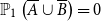 ${\mathbb P}_1\left (\overline {A} \cup \overline {B}\right )=0$
, and if
${\mathbb P}_1\left (\overline {A} \cup \overline {B}\right )=0$
, and if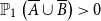 ${\mathbb P}_1\left (\overline {A} \cup \overline {B}\right ) \gt 0$
then (3.22) states that the average value of
${\mathbb P}_1\left (\overline {A} \cup \overline {B}\right ) \gt 0$
then (3.22) states that the average value of $|\phi (u)|$
on
$|\phi (u)|$
on $\overline {A} \cup \overline {B}$
does not exceed three times the average value of
$\overline {A} \cup \overline {B}$
does not exceed three times the average value of $|\phi (u)|$
on
$|\phi (u)|$
on $A \cap B$
, which follows from (3.21).
$A \cap B$
, which follows from (3.21).
Similarly, to pass from $\phi (u)$
to
$\phi (u)$
to $\widehat {\phi }(u)$
for
$\widehat {\phi }(u)$
for $u \in A$
, we change at most
$u \in A$
, we change at most $k-1$
in total functions
$k-1$
in total functions $h_i(\!\cdot | u)$
to
$h_i(\!\cdot | u)$
to $\widehat {h}_i(\!\cdot | u)$
and
$\widehat {h}_i(\!\cdot | u)$
and $f_i(y)$
to
$f_i(y)$
to $\widehat {f}_i(y)$
in (3.12), and hence applying Claim 2 of the induction hypothesis, we obtain
$\widehat {f}_i(y)$
in (3.12), and hence applying Claim 2 of the induction hypothesis, we obtain
 \begin{equation*}|\widehat {\phi }(u)| \ \leq \ \beta ^{k-1} |\phi (u)| \quad \text{for all} \quad u \in A \end{equation*}
and hence
 \begin{equation} \int _{A \cap B} |\widehat {\phi }(u)| \ du \ \leq \ \beta ^{k-1} \int _{A \cap B} | \phi (u)|\ du. \end{equation}
On the other hand, in $\widehat {\phi }(u_2)$
for
$\widehat {\phi }(u_2)$
for $u_2 \in {\mathbf \Omega _1}$
compared to
$u_2 \in {\mathbf \Omega _1}$
compared to $\phi (u_1)$
for
$\phi (u_1)$
for $u_1 \in A$
, we replace additionally up to
$u_1 \in A$
, we replace additionally up to $|I| \leq \Delta$
functions
$|I| \leq \Delta$
functions $h_i(\!\cdot |u_1)$
by
$h_i(\!\cdot |u_1)$
by $h_i(\!\cdot | u_2)$
, and so from Claim 2 of the induction hypothesis, we get
$h_i(\!\cdot | u_2)$
, and so from Claim 2 of the induction hypothesis, we get
 \begin{equation} \begin{aligned} |\widehat {\phi }(u_2)| \ \leq \ &\beta ^{k-1} \beta ^{|I|} |\phi (u_1)| \ \leq \ 3\beta ^{k-1} |\phi (u_1)| \\ &\text{for all} \quad u_1 \in A, \ u_2 \in {\mathbf \Omega _1}. \end{aligned} \end{equation}
It follows then that
 \begin{equation} \int _{\overline {A} \cup \overline {B}} |\widehat {\phi }(u)| \ du \ \leq \ 3 \beta ^{k-1} \frac {{\mathbb P}_1(\overline {A} \cup \overline {B})}{{\mathbb P}_1(A \cap B)} \int _{A \cap B} |\phi (u)| \ du. \end{equation}
Indeed, (3.25) obviously holds if ${\mathbb P}_1(\overline {A} \cup \overline {B})=0$
, and if
${\mathbb P}_1(\overline {A} \cup \overline {B})=0$
, and if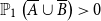 ${\mathbb P}_1\left (\overline {A} \cup \overline {B}\right ) \gt 0$
then (3.25) states that the average value of
${\mathbb P}_1\left (\overline {A} \cup \overline {B}\right ) \gt 0$
then (3.25) states that the average value of $|\widehat {\phi }(u)|$
on
$|\widehat {\phi }(u)|$
on $\overline {A} \cup \overline {B}$
does not exceed
$\overline {A} \cup \overline {B}$
does not exceed $3\beta ^{k-1}$
times the average value of
$3\beta ^{k-1}$
times the average value of $|\phi (u)|$
on
$|\phi (u)|$
on $A \cap B$
, which follows from (3.24).
$A \cap B$
, which follows from (3.24).
3.5
Induction step
$n-1 \Longrightarrow n$
, Claim 1

We compare the first two integrals in (3.13) and argue that the bulk of both integrals come from integrating over the event $A \cap B$
, for
$A \cap B$
, for $A$
defined by (3.15) and
$A$
defined by (3.15) and $B$
defined by (3.17), where the integrals obviously coincide. Indeed, by (3.17) we have
$B$
defined by (3.17), where the integrals obviously coincide. Indeed, by (3.17) we have
 \begin{equation*}\int _{A \cap B} f_n(u) \phi (u) \ du= \int _{A \cap B} \phi (u)\ du.\end{equation*}
From (3.13),
 \begin{equation} \left | \int _{\mathbf{\Omega }} \prod _{i=1}^n f_i(x) \ d x - \int _{A \cap B} \phi (u) \ du \right | \ \leq \ \int _{\overline {A} \cup \overline {B}} | f_n(u) \phi (u)| \ du \end{equation}
and similarly,
 \begin{equation} \left | \int _{\mathbf{\Omega }} \prod _{i=1}^{n-1} f_i(x) \ d x - \int _{A \cap B} \phi (u) \ du \right | \ \leq \ \int _{\overline {A} \cup \overline {B}} | \phi (u)| \ du. \end{equation}
Using (3.2), (3.22), (3.19), and (3.20) in that order, we conclude that
 \begin{equation} \begin{aligned} &\int _{\overline {A} \cup \overline {B}} |f_n(u) \phi (u)| \ d u \ \leq \ \left (1 + \frac {1}{6 \Delta }\right ) \int _{\overline {A} \cup \overline {B}} |\phi (u)| \ du \\ &\qquad \leq \ \left (1+ \frac {1}{6 \Delta }\right ) \frac { 3{\mathbb P}_1(\overline {A} \cup \overline {B})}{{\mathbb P}_1(A \cap B)} \int _{A \cap B} |\phi (u)| \ du \\ &\qquad \leq \ \left (1 + \frac {1}{6\Delta }\right ) \left (\frac {6}{\gamma ^3 \Delta ^2- 2 }\right ) \int _{A \cap B} |\phi (u)| \ du \\ &\qquad \leq \ \left (1 + \frac {1}{6\Delta }\right ) \left (\frac {6}{\gamma ^3 \Delta ^2 -2}\right )\left ( \frac {1}{\cos (1/\Delta )}\right ) \left | \int _{A \cap B} \phi (u) \ du \right |. \end{aligned} \end{equation}
and, similarly,
 \begin{equation} \int _{\overline {A} \cup \overline {B}} |\phi (u)| \ d u \ \leq \ \left (\frac {6}{\gamma ^3 \Delta ^2 -2}\right )\left ( \frac {1}{\cos (1/\Delta )}\right ) \left | \int _{A \cap B} \phi (u) \ du \right |. \end{equation}
In view of (3.26)–(3.29) and Lemma 4, to make sure that
 \begin{equation*}\int _{{\mathbf \Omega }} \prod _{i=1}^n f_i(x) \ dx \ne 0, \quad \int _{{\mathbf \Omega }} \prod _{i=1}^{n-1} f_i(x) \ dx \ne 0\end{equation*}
and that the angles between each of these two integrals and
 \begin{equation*} \int _{A \cap B} \phi (u) \ du \ \ne 0,\end{equation*}
cf. (3.20), do not exceed $\theta /2 = \frac {1}{2 \Delta ^2}$
each, we should make sure that
$\theta /2 = \frac {1}{2 \Delta ^2}$
each, we should make sure that
 \begin{equation} \left (1 + \frac {1}{6\Delta }\right ) \left (\frac {6}{\gamma ^3 \Delta ^2 -2}\right )\left ( \frac {1}{\cos (1/\Delta )}\right ) \ \leq \ \sin \frac {1}{2 \Delta ^2}. \end{equation}
Clearly, (3.30) holds for a sufficiently large $\gamma \gt 1$
. Computations show that (3.30) holds when
$\gamma \gt 1$
. Computations show that (3.30) holds when $\Delta \geq 3$
and
$\Delta \geq 3$
and $\gamma \geq 3$
, so Claim 1 holds.
$\gamma \geq 3$
, so Claim 1 holds.
3.6
Induction step
$n-1 \Longrightarrow n$
, Claim 2

Here we compare the first and the last integrals in (3.13), and once again argue that the main contribution to both come from the integral over the event $A \cap B$
, for
$A \cap B$
, for $A$
defined by (3.15) and
$A$
defined by (3.15) and $B$
defined by (3.17). From (3.13) and (3.2), we have
$B$
defined by (3.17). From (3.13) and (3.2), we have
 \begin{equation*} \begin{aligned} &\left | \int _{{\mathbf \Omega }} \left ( \prod _{i=1}^{n-k} f_i(x) \prod _{i=n-k+1}^n \widehat {f}_i(x) \right ) \ dx\right | = \left | \int _{{\mathbf \Omega _1}} \widehat {f}_n(u) \widehat {\phi }(u) \ du \right | \\ &\qquad \leq \ \left (1+ \frac {1}{6\Delta }\right ) \int _{{\mathbf \Omega _1}} |\widehat {\phi }(u)| \ du. \end{aligned} \end{equation*}
As before, the last integral we split into two cases: over $A \cap B$
and over
$A \cap B$
and over $\overline {A} \cup \overline {B}$
. Applying (3.2), (3.23), (3.25), and (3.20) in that order, we get
$\overline {A} \cup \overline {B}$
. Applying (3.2), (3.23), (3.25), and (3.20) in that order, we get
 \begin{equation*} \begin{aligned} &\left | \int _{{\mathbf \Omega _1}} \widehat {f}_n(u) \widehat {\phi }(u) \ du \right | \ \leq \ \left (1+ \frac {1}{6 \Delta }\right ) \left ( \int _{A \cap B} |\widehat {\phi }(u)| \ du + \int _{\overline {A} \cup \overline {B}} |\widehat {\phi }(u)| \ du \right ) \\ &\qquad \leq \ \beta ^{k-1} \left (1 + \frac {1}{6 \Delta }\right ) \left (1 + 3 \frac {{\mathbb P}_1(\overline {A} \cup \overline {B})}{{\mathbb P}_1(A \cap B)} \right ) \int _{A \cap B} |\phi (u)| \ du \\ &\qquad \leq \ \beta ^{k-1}\left (1+ \frac {1}{6 \Delta }\right ) \left (1+\frac {6}{\gamma ^3 \Delta ^2 -2}\right )\left ( \frac {1}{\cos (1/\Delta )}\right ) \left | \int _{A \cap B} \phi (u) \ du \right |\!. \end{aligned} \end{equation*}
It is clear now that for sufficiently large $\Delta \geq 1$
and
$\Delta \geq 1$
and $\gamma \gt 1$
, we have
$\gamma \gt 1$
, we have
 \begin{equation} \left (1+ \frac {1}{6 \Delta }\right ) \left (1+\frac {6}{\gamma ^3 \Delta ^2 -2}\right )\left ( \frac {1}{\cos (1/\Delta )}\right ) \ \leq \ 1 + \frac {1}{3 \Delta } \end{equation}
and computations show that (3.31) holds for $\Delta \geq 5$
and
$\Delta \geq 5$
and $\gamma \geq 3$
. Hence,
$\gamma \geq 3$
. Hence,
 \begin{equation} \begin{aligned} &\left | \int _{{\mathbf \Omega _1}} \widehat {f}_n(u) \widehat {\phi }(u) \ du \right | \ \leq \ \beta ^{k-1} \left (1 + \frac {1}{3 \Delta }\right ) \left | \int _{A \cap B} \phi (u) \ du\right | \\ &\qquad \text{provided} \quad \Delta \geq 5 \quad \text{and} \quad \gamma \geq 3. \end{aligned} \end{equation}
On the other hand, from (3.13) and (3.28),
 \begin{equation*} \begin{aligned} &\left | \int _{\Omega } \prod _{i=1}^n f_i(x) \ dx\right | = \left | \int _{{\mathbf \Omega _1}} f_n(u) \phi (u) \ du \right | \\ &\qquad \geq \ \left | \int _{A \cap B} \phi (u) \ du \right | - \left | \int _{\overline {A} \cup \overline {B}} f_n(u) \phi (u) \ du \right |\\ &\qquad \geq \ \left (1- \left (1 + \frac {1}{6\Delta }\right ) \left (\frac {6}{\gamma ^3 \Delta ^2 -2}\right )\left ( \frac {1}{\cos (1/\Delta )}\right )\right ) \left | \int _{A \cap B} \phi (u) \ du \right |. \end{aligned} \end{equation*}
It is now clear that if $\Delta \geq 1$
and
$\Delta \geq 1$
and $\gamma \geq 1$
are sufficiently large, then
$\gamma \geq 1$
are sufficiently large, then
 \begin{equation} \left (1+\frac {1}{6\Delta }\right ) \left (\frac {6}{\gamma ^3 \Delta ^2 -2}\right )\left ( \frac {1}{\cos (1/\Delta )}\right ) \ \leq \ \frac {1}{15 \Delta }. \end{equation}
Computations show that (3.33) indeed holds for $\Delta \geq 5$
and
$\Delta \geq 5$
and $\gamma \geq 3$
, so we have
$\gamma \geq 3$
, so we have
 \begin{equation} \begin{aligned} &\left | \int _{{\mathbf \Omega _1}} f_n(u) \phi (u) \ du \right | \ \geq \ \left (1 - \frac {1}{15 \Delta }\right ) \left | \int _{A\cap B} \phi (u) \ du \right | \\ &\quad \text{provided} \quad \Delta \geq 5 \quad \text{and} \quad \gamma \geq 3. \end{aligned} \end{equation}
Since for $\Delta \geq 5$
, we have
$\Delta \geq 5$
, we have
 \begin{equation*}\left ( 1+ \frac {1}{3 \Delta }\right ) \left (1- \frac {1}{15 \Delta }\right )^{-1} \ \lt \ 1+ \frac {1}{\Delta } =\beta ,\end{equation*}
combining (3.13), (3.32), and (3.34), we conclude that Claim 2 holds.
4. Concluding remarks
4.1 Comparison with the cluster expansion method
One can prove a version of Theorem 1 using the method of cluster expansion, see [Reference Jenssen, Fischer and Johnson14] for a survey. This method was also used by Bencs and Regts [Reference Bencs and G. Regts6] in the particular case of approximating the volume of a truncated independence polytope of a graph and then by Guo and N [Reference Guo and Vishvajeet11] to approximate the volume of a truncated matching polytope of a hypergraph. We briefly sketch how cluster expansion can work in the general framework of Theorem 1.
Given events $A_1, \ldots , A_n$
as in Theorem 1, we still consider the polynomial
$A_1, \ldots , A_n$
as in Theorem 1, we still consider the polynomial
 \begin{equation} \begin{aligned} p(z)=&\int _{{\mathbf \Omega }} \prod _{i=1}^n (1-z [A_i]) \ dx\\= &\sum _{k=0}^{n} (\!-\!1)^k z^k \sum _{1 \leq i_1 \lt \ldots \lt i_k \leq n} {\mathbb P}(A_{i_1} \cap \ldots \cap A_{i_k}) \end{aligned} \end{equation}
and aim to prove that $p(z) \ne 0$
in a neighbourhood of
$p(z) \ne 0$
in a neighbourhood of $[0, 1] \subset {\mathbb C}$
, see Sections 2.1 and 2.2. We construct a graph
$[0, 1] \subset {\mathbb C}$
, see Sections 2.1 and 2.2. We construct a graph $G=(V, E)$
with set
$G=(V, E)$
with set $V=\{1, \ldots , n\}$
of vertices, and vertices
$V=\{1, \ldots , n\}$
of vertices, and vertices $i$
and
$i$
and $j$
spanning an edge whenever
$j$
spanning an edge whenever $A_i$
and
$A_i$
and $A_j$
share a coordinate. The expansion (4.1) allows one to apply the polymer model here: for each collection
$A_j$
share a coordinate. The expansion (4.1) allows one to apply the polymer model here: for each collection $1 \leq i_1 \lt \ldots \lt i_k \leq n$
, we consider the subgraph
$1 \leq i_1 \lt \ldots \lt i_k \leq n$
, we consider the subgraph $H=H_{i_1, \ldots , i_k}$
of
$H=H_{i_1, \ldots , i_k}$
of $G$
induced by
$G$
induced by $i_1, \ldots , i_k$
and define its (complex) weight by
$i_1, \ldots , i_k$
and define its (complex) weight by
 \begin{equation*}w(H_{i_1, \ldots , i_k}) = (\!-\!1)^k z^k {\mathbb P}(A_{i_1} \cap \ldots \cap A_{i_k}).\end{equation*}
Then (4.1) is the sum of $w(H)$
over all induced subgraphs
$w(H)$
over all induced subgraphs $H$
of
$H$
of $G$
, including the empty subgraph with weight 1.
$G$
, including the empty subgraph with weight 1.
We say that two connected induced subgraphs $H_1$
and
$H_1$
and $H_2$
of
$H_2$
of $G$
are compatible, denoted
$G$
are compatible, denoted $H_1 \sim H_2$
, if they are vertex-disjoint and there are no vertices
$H_1 \sim H_2$
, if they are vertex-disjoint and there are no vertices $v_1$
of
$v_1$
of $H_1$
and
$H_1$
and $v_2$
of
$v_2$
of $H_2$
spanning an edge of
$H_2$
spanning an edge of $G$
, and incompatible, denoted
$G$
, and incompatible, denoted $H_1 \not \sim H_2$
, otherwise. The crucial property that makes the polymer model work is that if the induced subgraph
$H_1 \not \sim H_2$
, otherwise. The crucial property that makes the polymer model work is that if the induced subgraph $H$
is a union of pairwise compatible connected subgraphs, say
$H$
is a union of pairwise compatible connected subgraphs, say $H^1, \ldots , H^s$
, then
$H^1, \ldots , H^s$
, then
 \begin{equation*}w(H) = w(H^1) \cdots w(H^s).\end{equation*}
The Kotecký–Preiss condition [Reference Kotecký and Preiss17], see also [Reference Jenssen, Fischer and Johnson14] for a survey, then provides a sufficient condition for $p(z)$
to be non-zero: if one can assign non-negative real weights
$p(z)$
to be non-zero: if one can assign non-negative real weights $\psi (H) \geq 0$
to the induced subgraphs
$\psi (H) \geq 0$
to the induced subgraphs $H$
such that for every connected induced subgraph
$H$
such that for every connected induced subgraph $F$
of
$F$
of $G$
, we have
$G$
, we have
 \begin{equation} \sum _{H\,:\,\ H \not \sim F} |w(H)| e^{\psi (H)} \ \leq \ \psi (F), \end{equation}
where the sum is taken over all connected induced subgraphs of $G$
that are incompatible with
$G$
that are incompatible with $F$
, including
$F$
, including $F$
itself. One can bound
$F$
itself. One can bound $|w(H)|$
from above by arguing that the graph
$|w(H)|$
from above by arguing that the graph $H$
with
$H$
with $|H|$
vertices contains a subset of size at least
$|H|$
vertices contains a subset of size at least $|H|/(\Delta +1)$
, corresponding to mutually independent events. The condition (4.2) allows one to establish that
$|H|/(\Delta +1)$
, corresponding to mutually independent events. The condition (4.2) allows one to establish that $p(z) \ne 0$
in a disc
$p(z) \ne 0$
in a disc
 \begin{equation} \bigl \{ z \in {\mathbb C}\,:\, \quad |z| \lt \rho \bigr \} \end{equation}
of some radius $\rho \gt 0$
(one should choose
$\rho \gt 0$
(one should choose $\psi (H)$
to be proportional to the number
$\psi (H)$
to be proportional to the number $|H|$
of vertices in
$|H|$
of vertices in $H$
). The bound one gets from this approach is
$H$
). The bound one gets from this approach is
 \begin{equation} {\mathbb P}(A_i) \lt \Delta ^{-\gamma \Delta }, \end{equation}
for an absolute constant $\gamma \gt 0$
, which is more restrictive than the bound of Theorem 1. After the first version of this paper was posted as a preprint, Mann and Waite [Reference Mann and Waite22], among other results, obtained a similar to (4.4) bound, only they bounded
$\gamma \gt 0$
, which is more restrictive than the bound of Theorem 1. After the first version of this paper was posted as a preprint, Mann and Waite [Reference Mann and Waite22], among other results, obtained a similar to (4.4) bound, only they bounded $|w(H)|$
in terms of the chromatic number of
$|w(H)|$
in terms of the chromatic number of $H$
.
$H$
.
One reason why our inductive proof of Theorems 1 and 2 achieve less restrictive conditions than (4.4) is that we aim to prove that $p(z)$
has no zeros in some fixed, but otherwise arbitrarily small neighbourhood of
$p(z)$
has no zeros in some fixed, but otherwise arbitrarily small neighbourhood of $[0, 1] \subset {\mathbb C}$
, which is still sufficient to deduce Theorem 1 from, while the cluster expansion conditions ensure a stronger claim of
$[0, 1] \subset {\mathbb C}$
, which is still sufficient to deduce Theorem 1 from, while the cluster expansion conditions ensure a stronger claim of $p(z)$
having no zeros in a disc. In our case, for the disc (4.3) to contain a neighbourhood of
$p(z)$
having no zeros in a disc. In our case, for the disc (4.3) to contain a neighbourhood of $[0, 1]$
, we need to have
$[0, 1]$
, we need to have $\rho =1+\delta$
for some fixed
$\rho =1+\delta$
for some fixed $\delta \gt 0$
. If we modify our proof so that it works also for the disc (4.3), we would also arrive to (4.4), basically because the condition (2.3) that
$\delta \gt 0$
. If we modify our proof so that it works also for the disc (4.3), we would also arrive to (4.4), basically because the condition (2.3) that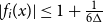 $|f_i(x)| \leq 1 + \frac {1}{6 \Delta }$
would have to be replaced by
$|f_i(x)| \leq 1 + \frac {1}{6 \Delta }$
would have to be replaced by $|f_i(x)| \leq 2 + \delta$
, which would require the values of
$|f_i(x)| \leq 2 + \delta$
, which would require the values of ${\mathbb P}(A_i)$
to be much smaller. On the other hand, one advantage of having the polynomial
${\mathbb P}(A_i)$
to be much smaller. On the other hand, one advantage of having the polynomial $p(z)$
to be non-zero in the disc (4.3) containing
$p(z)$
to be non-zero in the disc (4.3) containing $[0, 1]$
is that it allows one to improve the bound for
$[0, 1]$
is that it allows one to improve the bound for $K$
in Theorem 1 to
$K$
in Theorem 1 to $K=O(\ln (n/\epsilon ))$
, where the implicit constant in the ‘
$K=O(\ln (n/\epsilon ))$
, where the implicit constant in the ‘ $O$
’ notation is absolute.
$O$
’ notation is absolute.
In their approximation of the volume of the truncated hypergraph matching polytope, Guo and N proposed in [Reference Guo and Vishvajeet11] a different polymer model, where the underlying graph is bipartite, with the coordinates on one side matched to the events on the other side. It would be interesting to find out if the model extends to the general case treated in this paper, and if it does, what bounds on the probabilities of $A_i$
it gives.
$A_i$
it gives.
4.2 Optimality
It is unclear if the upper bound for ${\mathbb P}(A_i)$
in Theorem 1 needs to be exponentially small in
${\mathbb P}(A_i)$
in Theorem 1 needs to be exponentially small in $\mu _i$
. From the proof of Theorem 2, the exponential dependence arises because of the following phenomenon: even when an event
$\mu _i$
. From the proof of Theorem 2, the exponential dependence arises because of the following phenomenon: even when an event $A \subset {\mathbf \Omega }_1\times {\mathbf \Omega }_2$
has small probability, for some
$A \subset {\mathbf \Omega }_1\times {\mathbf \Omega }_2$
has small probability, for some $\omega _1 \in {\mathbf \Omega }_1$
, its section
$\omega _1 \in {\mathbf \Omega }_1$
, its section
 \begin{equation} A_{\omega _1}=\bigl \{ \omega _2 \in {\mathbf \Omega }_2\,:\, (\omega _1, \omega _2) \in A \bigr \} \end{equation}
may still have a large probability in ${\mathbf \Omega }_2$
. Since by the Markov inequality, the probability to hit such an
${\mathbf \Omega }_2$
. Since by the Markov inequality, the probability to hit such an $\omega _1 \in {\mathbf \Omega }_1$
cannot be too large, our inductive proof carries through, but the very existence of such
$\omega _1 \in {\mathbf \Omega }_1$
cannot be too large, our inductive proof carries through, but the very existence of such $\omega _1$
creates the exponential in
$\omega _1$
creates the exponential in $\mu _i$
dependence in our proof.
$\mu _i$
dependence in our proof.
When we have a better control over the probability of $A_{\omega _1}$
defined by (4.5), the bounds for
$A_{\omega _1}$
defined by (4.5), the bounds for ${\mathbb P}(A_i)$
improve. In particular, this happens if there is a non-trivial upper bound on
${\mathbb P}(A_i)$
improve. In particular, this happens if there is a non-trivial upper bound on ${\mathbb P}(A_{\omega _1})$
as long as
${\mathbb P}(A_{\omega _1})$
as long as $A_{\omega _1} \ne {\mathbf \Omega }_2$
. This is the case, for example, when each
$A_{\omega _1} \ne {\mathbf \Omega }_2$
. This is the case, for example, when each $\Omega _j$
is a finite subset of some field
$\Omega _j$
is a finite subset of some field $\mathbb F$
and each event
$\mathbb F$
and each event $A_i$
is defined by a polynomial equation. The analysis also becomes simpler, we sketch it in Section 4.3. We also note that in counting solutions to CNF Boolean formulas, hypergraph colourings or independent sets in hypergraphs, where better bounds are known, each event
$A_i$
is defined by a polynomial equation. The analysis also becomes simpler, we sketch it in Section 4.3. We also note that in counting solutions to CNF Boolean formulas, hypergraph colourings or independent sets in hypergraphs, where better bounds are known, each event $A_i \subset {\mathbf \Omega }$
has the structure of a direct product
$A_i \subset {\mathbf \Omega }$
has the structure of a direct product $A_i = A_i^1 \times \cdots \times A_i^m$
with
$A_i = A_i^1 \times \cdots \times A_i^m$
with $A_i^j \subset \Omega _j$
, cf. [Reference Bencs and Buys5], or a union of a small number of such products [Reference Galvin, McKinley, Perkins, Sarantis and Tetali9, Reference He, Wang and Yin12, Reference Jain, Pham and Vuong13, Reference Liu, Wang, Yin and Yu21, Reference Moitra23].
$A_i^j \subset \Omega _j$
, cf. [Reference Bencs and Buys5], or a union of a small number of such products [Reference Galvin, McKinley, Perkins, Sarantis and Tetali9, Reference He, Wang and Yin12, Reference Jain, Pham and Vuong13, Reference Liu, Wang, Yin and Yu21, Reference Moitra23].
On the other hand, the bounds obtained in [Reference Guo and Vishvajeet11] for ‘bad events’ $A_i$
in the problem of approximating the volumes of some combinatorially defined polytopes indeed appear to be exponentially small in
$A_i$
in the problem of approximating the volumes of some combinatorially defined polytopes indeed appear to be exponentially small in $\mu _i$
. More precisely, the bounds of [Reference Guo and Vishvajeet11], when stated in terms of our Theorem 1, appear to be
$\mu _i$
. More precisely, the bounds of [Reference Guo and Vishvajeet11], when stated in terms of our Theorem 1, appear to be ${\mathbb P}(A_i)=\Delta ^{-O(r)} r^{-O(r)}$
for
${\mathbb P}(A_i)=\Delta ^{-O(r)} r^{-O(r)}$
for $r=\max _{i=1, \ldots , n} r_i$
.
$r=\max _{i=1, \ldots , n} r_i$
.
4.3 A simpler case
Let $\Omega _1, \ldots , \Omega _m$
be probability spaces, let
$\Omega _1, \ldots , \Omega _m$
be probability spaces, let ${\mathbf \Omega } = \Omega _1 \times \ldots \times \Omega _m$
be their product, and let
${\mathbf \Omega } = \Omega _1 \times \ldots \times \Omega _m$
be their product, and let $A_1, \ldots , A_n \subset {\mathbf \Omega }$
. As in Section 2.2, we fix a
$A_1, \ldots , A_n \subset {\mathbf \Omega }$
. As in Section 2.2, we fix a $\delta$
-neighbourhood
$\delta$
-neighbourhood $U$
of the interval
$U$
of the interval $[0, 1] \subset {\mathbb C}$
and with a
$[0, 1] \subset {\mathbb C}$
and with a $z \in U$
, we associate a random variable
$z \in U$
, we associate a random variable $f_i\,:\, {\mathbf \Omega } \longrightarrow {\mathbb C}$
defined by
$f_i\,:\, {\mathbf \Omega } \longrightarrow {\mathbb C}$
defined by $f_i(x)=1-z[A_i]$
, so that
$f_i(x)=1-z[A_i]$
, so that
 \begin{equation} | f_i(x)| \ \leq \ 1+ \delta \quad \text{for all} \quad x \in {\mathbf \Omega }. \end{equation}
As before, we assume that each function $f_i$
shares a coordinate with at most
$f_i$
shares a coordinate with at most $\Delta$
other functions
$\Delta$
other functions $f_k$
.
$f_k$
.
We also make a stronger assumption as follows. As in Section 3.4, let us write ${\mathbf \Omega }={\mathbf \Omega }_1 \times {\mathbf \Omega }_2$
and
${\mathbf \Omega }={\mathbf \Omega }_1 \times {\mathbf \Omega }_2$
and ${\mathbb P}={\mathbb P}_1 \times {\mathbb P}_2$
, write
${\mathbb P}={\mathbb P}_1 \times {\mathbb P}_2$
, write $x \in {\mathbf \Omega }$
as
$x \in {\mathbf \Omega }$
as $x=(u, y)$
, where
$x=(u, y)$
, where $u \in {\mathbf \Omega }_1$
and
$u \in {\mathbf \Omega }_1$
and $y \in {\mathbf \Omega }_2$
, and for
$y \in {\mathbf \Omega }_2$
, and for $f_i$
and
$f_i$
and $u \in {\mathbf \Omega }_1$
, consider the restriction
$u \in {\mathbf \Omega }_1$
, consider the restriction $h_i(\!\cdot | u)\,:\, {\mathbf \Omega }_2 \longrightarrow {\mathbb C}$
. Now, we assume that for some
$h_i(\!\cdot | u)\,:\, {\mathbf \Omega }_2 \longrightarrow {\mathbb C}$
. Now, we assume that for some $0 \lt \rho \lt 1/(\Delta +1)$
, each
$0 \lt \rho \lt 1/(\Delta +1)$
, each $f_i$
and every
$f_i$
and every $u \in {\mathbf \Omega }_1$
, we have
$u \in {\mathbf \Omega }_1$
, we have
 \begin{equation} \begin{aligned} &{\mathbb P} (x \in {\mathbf \Omega }\,:\,\ f_i(x) \ne 1 ) \ \leq \ \rho \quad \text{and} \\ &{\mathbb P}_2(y \in {\mathbf \Omega }_2\,:\,\ h_i(y | u) \ne 1\ ) \ \leq \ \rho , \quad \text{unless $h_i(\!\cdot | u)$ is constant on ${\mathbf \Omega }_2$}. \end{aligned} \end{equation}
We assume that (4.7) holds with every decomposition ${\mathbf \Omega }={\mathbf \Omega _1} \times {\mathbf \Omega }_2$
.
${\mathbf \Omega }={\mathbf \Omega _1} \times {\mathbf \Omega }_2$
.
One particular example where (4.7) is satisfied is as follows. Suppose that $\Omega _1=\ldots = \Omega _m$
is a subset with
$\Omega _1=\ldots = \Omega _m$
is a subset with $q$
elements of some field
$q$
elements of some field $\mathbb F$
, each
$\mathbb F$
, each $\Omega _j$
endowed with the uniform probability measure, and suppose that each
$\Omega _j$
endowed with the uniform probability measure, and suppose that each $A_i$
is the set of solutions
$A_i$
is the set of solutions $\left (\xi _1, \ldots , \xi _m\right ) \in {\mathbf \Omega }$
to a polynomial equation of some degree
$\left (\xi _1, \ldots , \xi _m\right ) \in {\mathbf \Omega }$
to a polynomial equation of some degree $d \geq 1$
over
$d \geq 1$
over $\mathbb F$
. In this case, we can choose
$\mathbb F$
. In this case, we can choose $\rho =d/q$
in (4.7), which is known as the Schwartz–Zippel lemma [Reference Schwartz26], see also Theorem 6.13 in [Reference Lidl and Niederreiter18].
$\rho =d/q$
in (4.7), which is known as the Schwartz–Zippel lemma [Reference Schwartz26], see also Theorem 6.13 in [Reference Lidl and Niederreiter18].
We claim that if we choose $\delta =1/2\Delta$
in (4.6) then with
$\delta =1/2\Delta$
in (4.6) then with $\rho =\gamma /\Delta ^2$
in (4.7) for some absolute constant
$\rho =\gamma /\Delta ^2$
in (4.7) for some absolute constant $\gamma \gt 0$
, we have
$\gamma \gt 0$
, we have
 \begin{equation*}\int _{{\mathbf \Omega }} \prod _{i=1}^n f_i(x) \ dx \ne 0 \quad \text{for all} \quad z \in U. \end{equation*}
We sketch the argument below, leaving full detail to the reader, since the proof is very similar to that of Section 3, only that with (4.7) it simplifies a lot. We proceed by induction on $n$
, proving that
$n$
, proving that
 \begin{equation} \int _{{\mathbf \Omega }} \prod _{i=1}^n f_i(x) \ dx \ne 0, \quad \int _{{\mathbf \Omega }} \prod _{i=1}^{n-1} f_i(x) \ dx \ne 0, \end{equation}
the angle between the two complex numbers in (4.8), considered as non-zero vectors in ${\mathbb R}^2={\mathbb C}$
does not exceed some
${\mathbb R}^2={\mathbb C}$
does not exceed some $\theta \leq \pi /2\Delta$
, while the ratio of their absolute values (in either order) does not exceed some
$\theta \leq \pi /2\Delta$
, while the ratio of their absolute values (in either order) does not exceed some $\beta \geq 1+\delta$
.
$\beta \geq 1+\delta$
.
One can easily check that the base of the induction ( $n=1$
) holds when
$n=1$
) holds when
 \begin{equation*}\beta \ \geq \ \frac {1}{1- (2+\delta ) \rho } \quad \text{and} \quad \sin \theta \ \geq \ (2+\delta ) \rho .\end{equation*}
Suppose now that $n \gt 1$
. Let
$n \gt 1$
. Let $\left \{\xi _j\,:\, j \in J \right \}$
be the set of variables that
$\left \{\xi _j\,:\, j \in J \right \}$
be the set of variables that $f_n$
depends on. If
$f_n$
depends on. If $J=\emptyset$
, function
$J=\emptyset$
, function $f_n$
is a constant, necessarily equal to 1, and the assertion holds with any
$f_n$
is a constant, necessarily equal to 1, and the assertion holds with any $\beta \geq 1$
and any
$\beta \geq 1$
and any $\theta \geq 0$
. Assuming that
$\theta \geq 0$
. Assuming that $J \ne \emptyset$
, we split
$J \ne \emptyset$
, we split ${\mathbf \Omega }={\mathbf \Omega }_1 \times {\mathbf \Omega _2}$
by (3.10), write
${\mathbf \Omega }={\mathbf \Omega }_1 \times {\mathbf \Omega _2}$
by (3.10), write $x=(u, y)$
and define
$x=(u, y)$
and define $\phi \,:\, {\mathbf \Omega }_1 \longrightarrow {\mathbb C}$
by the first equation in (3.12), so that the first two equations in (3.13) hold. Next, similarly to Section 3.4, we define two events
$\phi \,:\, {\mathbf \Omega }_1 \longrightarrow {\mathbb C}$
by the first equation in (3.12), so that the first two equations in (3.13) hold. Next, similarly to Section 3.4, we define two events $A, B \subset {\mathbf \Omega }_1$
by
$A, B \subset {\mathbf \Omega }_1$
by
 \begin{align*} \begin{aligned} &A= \{u \in {\mathbf \Omega }_1\,: \quad {\mathbb P}_2\left (h_i(\!\cdot | u) \ne 1 \right ) \ \leq \ \rho \quad \text{for all} \quad i \in I \} \quad \text{and} \\ &B= \{ u \in {\mathbf \Omega }_1\,: \quad f_n(u) = 1 \}. \end{aligned} \end{align*}
As in Section 3.4, we argue that the bulk in both integrals (4.8) are supplied by the integral
 \begin{equation*}\int _{A \cap B} f_n(u) \phi (u) \ du = \int _{A \cap B} \phi (u) \ du.\end{equation*}
Clearly,
 \begin{equation} {\mathbb P}_1 (\overline {B} ) \ \leq \ \rho . \end{equation}
To bound ${\mathbb P}_1(\overline {A})$
, we observe that we can have
${\mathbb P}_1(\overline {A})$
, we observe that we can have ${\mathbb P}_2 (h_i(\!\cdot | u) \ne 1 ) \gt \rho$
only if
${\mathbb P}_2 (h_i(\!\cdot | u) \ne 1 ) \gt \rho$
only if $h_i(\!\cdot |u )$
is a constant other than 1 on
$h_i(\!\cdot |u )$
is a constant other than 1 on ${\mathbf \Omega }_2$
, in which case
${\mathbf \Omega }_2$
, in which case ${\mathbb P}_2 (h_i(\!\cdot | u) \ne 1 ) = 1$
. Since
${\mathbb P}_2 (h_i(\!\cdot | u) \ne 1 ) = 1$
. Since ${\mathbb P} (f_i(x) \ne 1 ) \leq \rho$
, we must have
${\mathbb P} (f_i(x) \ne 1 ) \leq \rho$
, we must have
 \begin{equation*}{\mathbb P}_1 \{ u \in {\mathbf \Omega }_1\,:\, {\mathbb P}_2 (h_i(\!\cdot | u) \ne 1 ) \gt \rho \} \ \leq \ \rho \quad \text{for all} \quad i \in I\end{equation*}
and hence
 \begin{equation} {\mathbb P}_1\left (\overline {A}\right ) \ \leq \ \Delta \rho . \end{equation}
Again, since all functions $h_i(\!\cdot | u)$
satisfying
$h_i(\!\cdot | u)$
satisfying ${\mathbb P}_2 (h_i(\!\cdot | u) \ne 1 ) \gt \rho$
are necessarily constants, in the absolute value not exceeding
${\mathbb P}_2 (h_i(\!\cdot | u) \ne 1 ) \gt \rho$
are necessarily constants, in the absolute value not exceeding $1+\delta$
, we can factor them out from the integral in (3.12) for
$1+\delta$
, we can factor them out from the integral in (3.12) for $\phi (u)$
and conclude by the induction hypothesis that
$\phi (u)$
and conclude by the induction hypothesis that
 \begin{equation} |\phi (u_1)| \ \leq \ \beta ^{2 \Delta } |\phi (u_2)| \quad \text{for all} \quad u_1 \in {\mathbf \Omega }_1 \quad \text{and all} \quad u_2 \in A. \end{equation}
As in Section 3.4, from the induction hypothesis we conclude that for any $u_1, u_2 \in A$
, the angle between any two complex numbers
$u_1, u_2 \in A$
, the angle between any two complex numbers $\phi (u_1)\ne 0$
and
$\phi (u_1)\ne 0$
and $\phi (u_2) \ne 0$
does not exceed
$\phi (u_2) \ne 0$
does not exceed $2 \Delta \theta$
and hence
$2 \Delta \theta$
and hence
 \begin{equation} \left | \int _{A \cap B} \phi (u) \ du \right | \ \geq \ \left ( \cos \Delta \theta \right ) \int _{A \cap B} |\phi (u)| \ du. \end{equation}
Finally, as in Section 3, combining (3.13) and (4.9)–(4.12), we conclude that the induction can proceed provided
 \begin{equation*}\frac {\beta -1}{\beta +1} \ \geq \ \frac {\rho (\Delta +1) \beta ^{2\Delta +1}}{(1-\rho (\Delta +1)) \cos (\Delta \theta )} \quad \text{and} \quad \sin \frac {\theta }{2} \ \geq \ \frac {\rho ( \Delta +1) \beta ^{2\Delta +1}}{\left (1-\rho (\Delta +1)\right ) \cos (\Delta \theta )}, \end{equation*}
(we leave the details to the reader).
Let us choose
 \begin{equation*}\theta = \delta = \frac {1}{2\Delta } \quad \text{and} \quad \beta =1+\frac {1}{\Delta }.\end{equation*}
It follows then that the induction can proceed if in (4.7), we have $\rho =\gamma /\Delta ^2$
for some absolute constant
$\rho =\gamma /\Delta ^2$
for some absolute constant $\gamma \gt 0$
.
$\gamma \gt 0$
.
Acknowledgements
The author is grateful to the anonymous referees for their careful reading of the paper and several suggestions to improve the presentation, and, in particular, for the suggestion to look for a special structure of the events $A_i$
that may improve general bounds.
$A_i$
that may improve general bounds.

 Open access

