


1. Introduction
A sequence $d_1\le \cdots \le d_n$
is graphical if there is a graph on
$d_1\le \cdots \le d_n$
is graphical if there is a graph on $n$
vertices with this degree sequence. The criteria under which sequences are graphical are well-known; see Havel [Reference Havel11], Hakimi [Reference Hakimi10], and Erdős and Gallai [Reference Erdős and Gallai7]. Recently, Balister, the second author, Groenland, Johnston, and Scott [Reference Balister, Donderwinkel, Groenland, Johnston and Scott2] showed that the number
$n$
vertices with this degree sequence. The criteria under which sequences are graphical are well-known; see Havel [Reference Havel11], Hakimi [Reference Hakimi10], and Erdős and Gallai [Reference Erdős and Gallai7]. Recently, Balister, the second author, Groenland, Johnston, and Scott [Reference Balister, Donderwinkel, Groenland, Johnston and Scott2] showed that the number $\mathcal{G}_n$
of such sequences satisfies
$\mathcal{G}_n$
of such sequences satisfies $n^{3/4}\mathcal{G}_n/4^n\to C$
. The constant
$n^{3/4}\mathcal{G}_n/4^n\to C$
. The constant $C$
is expressed as a certain random walk probability
$C$
is expressed as a certain random walk probability $\rho$
; see (4) below.
$\rho$
; see (4) below.
In this work, we show that $C$
can be expressed in terms of the number
$C$
can be expressed in terms of the number $\mathcal{T}_n$
of rooted unlabelled plane trees with
$\mathcal{T}_n$
of rooted unlabelled plane trees with $n$
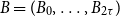
edges. Note that, in counting such trees, two trees are equivalent if one can be transformed into the other by cyclically permuting its subtrees about the root; see Figure 1 below. Using Pólya’s enumeration theorem, Walkup [Reference Walkup19] showed that
$n$
edges. Note that, in counting such trees, two trees are equivalent if one can be transformed into the other by cyclically permuting its subtrees about the root; see Figure 1 below. Using Pólya’s enumeration theorem, Walkup [Reference Walkup19] showed that
 \begin{align} \mathcal{T}_n = \frac {1}{n} \sum _{d|n}\binom{2d-1}{d}\phi (n/d),\end{align}
where $\phi (n)$
is Euler’s totient function. Our main result reveals the following connection between plane trees and graphical sequences.
$\phi (n)$
is Euler’s totient function. Our main result reveals the following connection between plane trees and graphical sequences.
Theorem 1.1.
As $n\to \infty$
, we have that
$n\to \infty$
, we have that
 \begin{align} \frac {n^{3/4}}{4^n} \mathcal{G}_n \to \frac {\Gamma (3/4)}{2^{5/2}\pi }e^\omega , \end{align}
where
 \begin{equation} \omega =\sum _{k=1}^\infty \frac {\mathcal{T}_k}{k4^k}. \end{equation}
Above, as usual, $\Gamma (z)=\int _0^\infty t^{z-1}e^{-t}dt$
is the gamma function. We call
$\Gamma (z)=\int _0^\infty t^{z-1}e^{-t}dt$
is the gamma function. We call $\omega$
Walkup’s constant.
$\omega$
Walkup’s constant.
The formula (1) can be used to numerically approximate the limiting constant on the right-hand side in (2); see (6) below.
The proof of Theorem1.1 involves an interplay between additive number theory, random walks, and renewal theory. The connection with number theory arises through a subset counting formula by von Sterneck (see, e.g., [Reference Bachmann1, Reference Ramanathan16]), which shows that $\mathcal{T}_n$
as in (1) coincides with the number of submultisets of
$\mathcal{T}_n$
as in (1) coincides with the number of submultisets of $\{0,1,\ldots ,n-1\}$
of size
$\{0,1,\ldots ,n-1\}$
of size $n$
that sum to
$n$
that sum to $0$
mod
$0$
mod $n$
. As we will see, this will allow us to relate plane trees to lattice paths (random walk trajectories). The connection between random walks and graphical sequences was observed in [Reference Balister, Donderwinkel, Groenland, Johnston and Scott2] (similar to the lattice path representation of tournament score sequences observed by Erdős and Moser; see, e.g., Moon [Reference Moon14]). In studying the random walks related to graphical sequences, we will use limit theory developed by Hawkes and Jenkins [Reference Hawkes and Jenkins12] (cf. Embrechts and Hawkes [Reference Embrechts and Hawkes6]) for infinitely divisible sequences (of which renewal sequences are a special case) related to the Lévy–Khintchine formula from the theory of Lévy processes. See Sections 1.2 and 2 below for more details.
$n$
. As we will see, this will allow us to relate plane trees to lattice paths (random walk trajectories). The connection between random walks and graphical sequences was observed in [Reference Balister, Donderwinkel, Groenland, Johnston and Scott2] (similar to the lattice path representation of tournament score sequences observed by Erdős and Moser; see, e.g., Moon [Reference Moon14]). In studying the random walks related to graphical sequences, we will use limit theory developed by Hawkes and Jenkins [Reference Hawkes and Jenkins12] (cf. Embrechts and Hawkes [Reference Embrechts and Hawkes6]) for infinitely divisible sequences (of which renewal sequences are a special case) related to the Lévy–Khintchine formula from the theory of Lévy processes. See Sections 1.2 and 2 below for more details.
The $\mathcal{T}_3=4$
rooted unlabelled plane trees with 3 edges.
$\mathcal{T}_3=4$
rooted unlabelled plane trees with 3 edges.

Figure 1 Long description
The image displays four distinct rooted unlabelled plane trees, each consisting of three edges. The trees are arranged in a vertical orientation, with each tree having a unique structure. The first tree is a straight vertical line with three nodes connected by two edges. The second tree has a central node branching into two nodes above it and one node below. The third tree features a central node with one node above it and two nodes below. The fourth tree has a central node with one node above it and two nodes branching out below it.
1.1 Degree sequences, via random walks
As already mentioned, Erdős and Moser observed a connection between random walks and degree sequences in the context of graph tournaments. A similar connection with random walks is used in [Reference Balister, Donderwinkel, Groenland, Johnston and Scott2] to show that
 \begin{equation} \frac {n^{3/4}}{4^n} \mathcal{G}_n\to \frac {\Gamma (3/4)}{2^{5/2}\pi } \frac {1}{\sqrt {1-\rho }}, \end{equation}
where $\rho$
is defined as follows.
$\rho$
is defined as follows.
Let $(Y_k,k\ge 0)$
be a lazy simple symmetric random walk, started at
$(Y_k,k\ge 0)$
be a lazy simple symmetric random walk, started at $Y_0=0$
, with increments
$Y_0=0$
, with increments $Y_{k+1}-Y_k$
equal to
$Y_{k+1}-Y_k$
equal to $\pm 1$
with probability
$\pm 1$
with probability $1/4$
, and
$1/4$
, and $0$
with probability
$0$
with probability $1/2$
. Let
$1/2$
. Let
 \begin{equation*} \tau =\inf \{k\ge 1 \, : \, Y_k=0,\: A_k\le 0\}, \end{equation*}
where $A_k=\sum _{i=1}^k Y_i$
is the area after
$A_k=\sum _{i=1}^k Y_i$
is the area after $k$
steps. Then
$k$
steps. Then
 \begin{equation} \rho =\textbf {P}(A_\tau =0). \end{equation}
In proving Theorem1.1, we obtain the following description of $\rho$
, in terms of Walkup’s constant
$\rho$
, in terms of Walkup’s constant $\omega$
.
$\omega$
.
Theorem 1.2.
We have that $\rho =1-e^{-2\omega }$
.
$\rho =1-e^{-2\omega }$
.
We note that Theorem1.1 follows by combining Theorem1.2 with (4).
1.2 Proof overview
There is a natural representation of the lazy simple symmetric random walk $(Y_k,0\le k\le n)$
in terms of a simple symmetric random walk
$(Y_k,0\le k\le n)$
in terms of a simple symmetric random walk $(X_k,0\le k\le 2n)$
of twice the length. In this representation, the area process is
$(X_k,0\le k\le 2n)$
of twice the length. In this representation, the area process is $A_k=\sum _{i=1}^k Y_i=\frac {1}{2}\sum _{i=1}^k X_{2i}$
. This relationship has a geometric interpretation; see the diamond area discussed in Section 3 below.
$A_k=\sum _{i=1}^k Y_i=\frac {1}{2}\sum _{i=1}^k X_{2i}$
. This relationship has a geometric interpretation; see the diamond area discussed in Section 3 below.
If $X_{2n}=0$
and
$X_{2n}=0$
and $A_k \ge 0$
at all times
$A_k \ge 0$
at all times $0\le k\le n$
for which
$0\le k\le n$
for which $X_{2k}=0$
, we call
$X_{2k}=0$
, we call $(X_k,0\le k\le 2n)$
a graphical walk of length
$(X_k,0\le k\le 2n)$
a graphical walk of length $2n$
. A graphical bridge is a graphical walk whose area returns to
$2n$
. A graphical bridge is a graphical walk whose area returns to $0$
at the end of its trajectory, and a graphical meander is a graphical walk whose area never returns to
$0$
at the end of its trajectory, and a graphical meander is a graphical walk whose area never returns to $0$
. Times
$0$
. Times $k$
when
$k$
when $X_{2k}=A_k=0$
play the role of renewal times, since initially
$X_{2k}=A_k=0$
play the role of renewal times, since initially $X_0=A_0=0$
. Hence a graphical walk can be decomposed into a series of graphical bridges and one final graphical meander. That is, the sequence
$X_0=A_0=0$
. Hence a graphical walk can be decomposed into a series of graphical bridges and one final graphical meander. That is, the sequence $(\mathcal{W}_n,n\ge 1)$
, where
$(\mathcal{W}_n,n\ge 1)$
, where $\mathcal{W}_n$
is the number of graphical walks of length
$\mathcal{W}_n$
is the number of graphical walks of length $2n$
, is a delayed renewal sequence, where the length of the final meander can be understood as the ‘delay’.
$2n$
, is a delayed renewal sequence, where the length of the final meander can be understood as the ‘delay’.
The term $\Gamma (3/4)/2^{5/2}\pi$
in (4) is related to the number of graphical meanders. In this work, to describe the other term
$\Gamma (3/4)/2^{5/2}\pi$
in (4) is related to the number of graphical meanders. In this work, to describe the other term $1/\sqrt {1-\rho }$
appearing in (4), we analyse the renewal sequence (without a delay)
$1/\sqrt {1-\rho }$
appearing in (4), we analyse the renewal sequence (without a delay) $(\mathcal{B}_n,n\ge 1)$
, where
$(\mathcal{B}_n,n\ge 1)$
, where $\mathcal{B}_n$
is the number of graphical bridges of length
$\mathcal{B}_n$
is the number of graphical bridges of length $2n$
. See Sections 2.1 and 2.2 below for more on renewal sequences, and Section 2.3 for more on their connection to the enumeration of
$2n$
. See Sections 2.1 and 2.2 below for more on renewal sequences, and Section 2.3 for more on their connection to the enumeration of $\mathcal{G}_n$
.
$\mathcal{G}_n$
.
To study the asymptotics of $\mathcal{B}_n$
, we use the asymptotic transference theory, developed by Hawkes and Jenkins [Reference Hawkes and Jenkins12] (cf. Embrechts and Hawkes [Reference Embrechts and Hawkes6]), for infinitely divisible distributions. We call this method the Lévy–Khintchine method (see Section 2 below), as it is related to the Lévy–Khintchine transform, which associates each such distribution with a corresponding Lévy process, via another measure called its Lévy measure. We show that the Lévy–Khintchine transform
$\mathcal{B}_n$
, we use the asymptotic transference theory, developed by Hawkes and Jenkins [Reference Hawkes and Jenkins12] (cf. Embrechts and Hawkes [Reference Embrechts and Hawkes6]), for infinitely divisible distributions. We call this method the Lévy–Khintchine method (see Section 2 below), as it is related to the Lévy–Khintchine transform, which associates each such distribution with a corresponding Lévy process, via another measure called its Lévy measure. We show that the Lévy–Khintchine transform $\mathcal{B}_n^*$
of
$\mathcal{B}_n^*$
of $\mathcal{B}_n$
is related to
$\mathcal{B}_n$
is related to $\mathcal{T}_n$
. In fact,
$\mathcal{T}_n$
. In fact, $\mathcal{B}_n^*=2\mathcal{T}_n$
. More specifically, we find that
$\mathcal{B}_n^*=2\mathcal{T}_n$
. More specifically, we find that $p_n=e^{-2\omega }\mathcal{B}^n/4^n$
is an infinitely divisible probability distribution with Lévy measure
$p_n=e^{-2\omega }\mathcal{B}^n/4^n$
is an infinitely divisible probability distribution with Lévy measure $\nu _n=2\mathcal{T}_n/n4^n$
. The measure
$\nu _n=2\mathcal{T}_n/n4^n$
. The measure $\nu _n$
is regularly varying, and it then follows by [Reference Hawkes and Jenkins12] that
$\nu _n$
is regularly varying, and it then follows by [Reference Hawkes and Jenkins12] that $p_n\sim \nu _n$
.
$p_n\sim \nu _n$
.
Our proof that $\mathcal{B}_n^*=2\mathcal{T}_n$
uses a characterisation of the Lévy–Khintchine transform of renewal sequences; see Lemma2.1 below. The proof also involves some combinatorial arguments: roughly speaking, by interleaving the steps of certain lattice paths, we relate the set of cyclical shifts of graphical bridges and the set of rooted plane trees. Our bijective arguments are geometric, using the diamond area; see Figs. 2, 3, 4, 5 and 6.
$\mathcal{B}_n^*=2\mathcal{T}_n$
uses a characterisation of the Lévy–Khintchine transform of renewal sequences; see Lemma2.1 below. The proof also involves some combinatorial arguments: roughly speaking, by interleaving the steps of certain lattice paths, we relate the set of cyclical shifts of graphical bridges and the set of rooted plane trees. Our bijective arguments are geometric, using the diamond area; see Figs. 2, 3, 4, 5 and 6.
Since $\mathcal{B}_n$
is a renewal sequence,
$\mathcal{B}_n$
is a renewal sequence, $\nu _n$
is also the harmonic renewal measure associated with the sequence
$\nu _n$
is also the harmonic renewal measure associated with the sequence $\mathcal{B}_n^{(1)}$
of irreducible graphical bridges. Using this, it follows that
$\mathcal{B}_n^{(1)}$
of irreducible graphical bridges. Using this, it follows that $e^{-2\omega }\nu _n/p_n$
is the harmonic moment
$e^{-2\omega }\nu _n/p_n$
is the harmonic moment $\textbf {E}[1/\mathcal{I}_n]$
of the number
$\textbf {E}[1/\mathcal{I}_n]$
of the number $\mathcal{I}_n$
of irreducible graphical bridges in a uniformly random graphical bridge of length
$\mathcal{I}_n$
of irreducible graphical bridges in a uniformly random graphical bridge of length $n$
and therefore
$n$
and therefore $\textbf {E}[1/\mathcal{I}_n]\to e^{-2\omega }$
(since
$\textbf {E}[1/\mathcal{I}_n]\to e^{-2\omega }$
(since $p_n\sim \nu _n$
).
$p_n\sim \nu _n$
).
Moreover, it can be shown that $\mathcal{I}_n$
converges to a negative binomial with parameters
$\mathcal{I}_n$
converges to a negative binomial with parameters $r=2$
and
$r=2$
and $p=1-\rho$
. Intuitively, renewal times will only occur near the start and end of the bridge. The numbers of such times on either side of the bridge are approximately independent and geometric with
$p=1-\rho$
. Intuitively, renewal times will only occur near the start and end of the bridge. The numbers of such times on either side of the bridge are approximately independent and geometric with $p=1-\rho$
. Therefore,
$p=1-\rho$
. Therefore, $\textbf {E}[1/\mathcal{I}_n]\to 1-\rho$
, and so we find that
$\textbf {E}[1/\mathcal{I}_n]\to 1-\rho$
, and so we find that $1-\rho =e^{-2\omega }$
, yielding Theorem1.2. Hence,
$1-\rho =e^{-2\omega }$
, yielding Theorem1.2. Hence, $1/\sqrt {1-\rho }=e^\omega$
, and so Theorem1.1 follows by (4).
$1/\sqrt {1-\rho }=e^\omega$
, and so Theorem1.1 follows by (4).
1.3 Ordered graphical sequences
The polytope $D_n$
of degree sequences was introduced by Koren [Reference Koren13] and studied by Peled and Srinivasan [Reference Peled and Srinivasan15]. Stanley [Reference Stanley18, Corollary 3.4] found a formula for the number of lattice points in
$D_n$
of degree sequences was introduced by Koren [Reference Koren13] and studied by Peled and Srinivasan [Reference Peled and Srinivasan15]. Stanley [Reference Stanley18, Corollary 3.4] found a formula for the number of lattice points in $D_n\cap \textbf {Z}^n$
with even sum, expressed in terms of quasi-forests. Such points are associated with ordered graphical sequences
$D_n\cap \textbf {Z}^n$
with even sum, expressed in terms of quasi-forests. Such points are associated with ordered graphical sequences $d_1,\ldots ,d_n$
. On the other hand, Theorem1.1 relates the number of unordered graphical sequences
$d_1,\ldots ,d_n$
. On the other hand, Theorem1.1 relates the number of unordered graphical sequences $d_1\le \cdots \le d_n$
and Walkup’s plane trees.
$d_1\le \cdots \le d_n$
and Walkup’s plane trees.
1.4 Numerics
Finally, let us note that the expression for $C$
in Theorem1.1 can be used to approximate
$C$
in Theorem1.1 can be used to approximate $\mathcal{G}_n$
, for large
$\mathcal{G}_n$
, for large $n$
. Observing that the formula (1) for
$n$
. Observing that the formula (1) for $\mathcal{T}_n$
is dominated by the
$\mathcal{T}_n$
is dominated by the $d=n$
term, one can show that
$d=n$
term, one can show that
 \begin{equation} \frac {n^{3/4}}{4^n}\mathcal{G}_n \to C \approx 0.099094083237488745361449340935. \end{equation}
See the discussion of this work in [Reference Balister, Donderwinkel, Groenland, Johnston and Scott2] for more details.
2. The Lévy–Khintchine method
A random variable $X$
is infinitely divisible if, for all
$X$
is infinitely divisible if, for all $n\ge 1$
, there are independent and identically distributed
$n\ge 1$
, there are independent and identically distributed $X_i$
such that
$X_i$
such that $\sum _{i=1}^n X_i$
and
$\sum _{i=1}^n X_i$
and $X$
are equal in distribution (see, e.g., [Reference Feller8]).
$X$
are equal in distribution (see, e.g., [Reference Feller8]).
Suppose that a positive sequence $(1=a_0,a_1,\ldots )$
is summable, so that it is proportional to a probability distribution
$(1=a_0,a_1,\ldots )$
is summable, so that it is proportional to a probability distribution $(\pi _n,n\ge 0)$
on the non-negative integers
$(\pi _n,n\ge 0)$
on the non-negative integers $n\ge 0$
. As is well-known (see, e.g., [Reference Hawkes and Jenkins12]) such a
$n\ge 0$
. As is well-known (see, e.g., [Reference Hawkes and Jenkins12]) such a $(\pi _n,n\ge 0)$
is infinitely divisible if and only if, for some non-negative sequence
$(\pi _n,n\ge 0)$
is infinitely divisible if and only if, for some non-negative sequence $(a^*_1, a^*_2,\ldots )$
, we have that
$(a^*_1, a^*_2,\ldots )$
, we have that
 \begin{equation} \sum _{n=0}^\infty a_n x^n =\exp \left (\sum _{k=1}^\infty \frac {a^*_k}{k}x^k\right ). \end{equation}
In this case, we call $(a_0,a_1,\ldots )$
an infinitely divisible sequence. By taking
$(a_0,a_1,\ldots )$
an infinitely divisible sequence. By taking $\log$
s and differentiating with respect to
$\log$
s and differentiating with respect to $x$
on both sides of (7) and then comparing coefficients, we see that (7) is equivalent to the recursion
$x$
on both sides of (7) and then comparing coefficients, we see that (7) is equivalent to the recursion
 \begin{equation} na_n =\sum _{i=1}^n a^*_i a_{n-i}, \quad \quad n\ge 1. \end{equation}
Since, as discussed in [Reference Embrechts and Hawkes6], (7) is a special case of the Lévy–Khintchine formula, we call $a_n^*$
the Lévy–Khintchine transform of
$a_n^*$
the Lévy–Khintchine transform of $a_n$
. We note that, in fact,
$a_n$
. We note that, in fact, $(\nu _n=a^*_n/n,n\ge 1)$
is the Lévy measure (see, e.g., [Reference Bertoin4]) associated with the Lévy process
$(\nu _n=a^*_n/n,n\ge 1)$
is the Lévy measure (see, e.g., [Reference Bertoin4]) associated with the Lévy process $(\mathcal{L}_t:t\ge 0)$
, for which the law of the process
$(\mathcal{L}_t:t\ge 0)$
, for which the law of the process $\mathcal{L}_1$
at time
$\mathcal{L}_1$
at time $t=1$
is described by the infinitely divisible probability measure
$t=1$
is described by the infinitely divisible probability measure
 \begin{equation*} \pi _n =a_n\exp \left (-\sum _{k=1}^\infty \frac {a^*_k}{k}\right ), \quad \quad n\ge 0. \end{equation*}
In combinatorial settings, it is convenient to consider $a_n=A_n/\alpha ^n$
, where
$a_n=A_n/\alpha ^n$
, where $A_n$
enumerates a class of objects of size
$A_n$
enumerates a class of objects of size $n$
that has exponential growth rate
$n$
that has exponential growth rate $\alpha$
. If
$\alpha$
. If $a_n$
is infinitely divisible, then
$a_n$
is infinitely divisible, then $A_n$
and
$A_n$
and $A^*_n=\alpha ^n a_n^*$
also satisfy (7) and (8), and naturally we also call
$A^*_n=\alpha ^n a_n^*$
also satisfy (7) and (8), and naturally we also call $A^*_n$
the Lévy–Khintchine transform of
$A^*_n$
the Lévy–Khintchine transform of $A_n$
.
$A_n$
.
A positive sequence $\vartheta (n)$
is regularly varying, with index
$\vartheta (n)$
is regularly varying, with index $\gamma$
, if
$\gamma$
, if
 \begin{equation*} \lim _{n\to \infty }\frac {\vartheta (\lfloor xn\rfloor )}{\vartheta (n)} =x^\gamma , \quad \quad \forall x\gt 0. \end{equation*}
One of our main tools for studying the asymptotics of sequences with a Lévy–Khintchine transform is a result by Hawkes and Jenkins [Reference Hawkes and Jenkins12], which shows that, if $a_n^*$
is regularly varying with some index
$a_n^*$
is regularly varying with some index $\gamma \lt 0$
, then
$\gamma \lt 0$
, then
 \begin{equation} a_n \sim \frac {a_n^*}{n} \exp \left (\sum _{k=1}^\infty \frac {a^*_k}{k}\right ). \end{equation}
In other words, in terms of the underlying Lévy process, the associated infinitely divisible probability measure $\pi _n$
and its corresponding Lévy measure
$\pi _n$
and its corresponding Lévy measure $\nu _n$
are asymptotically equivalent,
$\nu _n$
are asymptotically equivalent, $\pi _n\sim \nu _n$
as
$\pi _n\sim \nu _n$
as $n\to \infty$
. This is related to the well-known one big jump principle in Lévy process theory.
$n\to \infty$
. This is related to the well-known one big jump principle in Lévy process theory.
2.1 Renewal sequences
A subfamily of sequences $(A_n,n\ge 0)$
that have a Lévy–Khintchine transform is the class of renewal sequences. See, e.g., Feller [Reference Feller8, Section XIII] for background information on renewal theory.
$(A_n,n\ge 0)$
that have a Lévy–Khintchine transform is the class of renewal sequences. See, e.g., Feller [Reference Feller8, Section XIII] for background information on renewal theory.
Definition 2.1. We call a sequence $(A_n,n\ge 0)$
a renewal sequence if its generating function
$(A_n,n\ge 0)$
a renewal sequence if its generating function $A(x)=\sum _{n\ge 1} A_n x^n$
can be written as
$A(x)=\sum _{n\ge 1} A_n x^n$
can be written as
 \begin{equation*} A(x)=\frac {1}{1-A^{(1)}(x)}, \end{equation*}
where $A^{(1)}(x)=\sum _{n\ge 0} A^{(1)}_n x^n$
is the generating function of some other sequence
$A^{(1)}(x)=\sum _{n\ge 0} A^{(1)}_n x^n$
is the generating function of some other sequence $(A^{(1)}_n,n\ge 0)$
.
$(A^{(1)}_n,n\ge 0)$
.
In combinatorics, such a sequence often arises when $A_n$
counts the number of some type of structures of length
$A_n$
counts the number of some type of structures of length $n$
, each of which can be decomposed into a series of irreducible parts. In this context,
$n$
, each of which can be decomposed into a series of irreducible parts. In this context, $A^{(1)}_n$
counts the number of irreducible structures of length
$A^{(1)}_n$
counts the number of irreducible structures of length $n$
.
$n$
.
It is well known (see, e.g., [Reference Hawkes and Jenkins12, p. 66]) that renewal sequences are infinitely divisible. In our recent work, we show that, if $(A_n,n\ge 0)$
is a renewal sequence then the Lévy–Khintchine transform
$(A_n,n\ge 0)$
is a renewal sequence then the Lévy–Khintchine transform $A^*_n$
of
$A^*_n$
of $A_n$
takes a special form.
$A_n$
takes a special form.
Lemma 2.1 [Reference Bassan, Donderwinkel and Kolesnik3, Lemma 2]. If $(A_n,n\ge 0)$
is a renewal sequence then
$(A_n,n\ge 0)$
is a renewal sequence then
-
(1) the Lévy–Khintchine transform $A_n^*$
of
$A_n$
is the number of pairs
$(X,m)$
, where
$X$
is a structure of length
$n$
and
$0\le m \lt \ell$
, where
$\ell =\ell (X)$
is the length of the first irreducible part of
$X$
, and
$A_n^*$
of
$A_n$
is the number of pairs
$(X,m)$
, where
$X$
is a structure of length
$n$
and
$0\le m \lt \ell$
, where
$\ell =\ell (X)$
is the length of the first irreducible part of
$X$
, and
-
(2) we have that
(10)where
\begin{equation} \frac {A_n^*}{nA_n} =\mathbf{E}\left [ \frac {1}{\mathcal{I}_n} \right ], \end{equation}
$\mathcal{I}_n$
is the number of irreducible parts in a uniformly random structure of length
$n$
.


We note that, in terms of the underlying Lévy process, the formula (10) says that, when $(A_n,n\ge 0)$
is a renewal sequence with growth rate
$(A_n,n\ge 0)$
is a renewal sequence with growth rate $\alpha$
, the Lévy measure
$\alpha$
, the Lévy measure $\nu _n=A_n^*/n\alpha ^n$
is the harmonic renewal measure (see, e.g., [Reference Greenwood, Omey and Teugels9]) associated with the measure
$\nu _n=A_n^*/n\alpha ^n$
is the harmonic renewal measure (see, e.g., [Reference Greenwood, Omey and Teugels9]) associated with the measure $\mu _n=A_n^{(1)}/\alpha ^n$
.
$\mu _n=A_n^{(1)}/\alpha ^n$
.
Remark 2.1. With Lemma 2.1 in hand, one can use (9) to obtain the asymptotics of a renewal sequence $(A_n,n\ge 1)$
using its Lévy–Khintchine transform
$(A_n,n\ge 1)$
using its Lévy–Khintchine transform $A^*_n$
, provided that there exists an
$A^*_n$
, provided that there exists an $\alpha \gt 0$
for which
$\alpha \gt 0$
for which $A^*_n/\alpha ^n$
is regularly varying with some index
$A^*_n/\alpha ^n$
is regularly varying with some index $\gamma \lt 0$
. In our experience, the sequence
$\gamma \lt 0$
. In our experience, the sequence $A^*_n$
tends to be more tractable than
$A^*_n$
tends to be more tractable than $A_n$
itself, and this lies at the core of the method.
$A_n$
itself, and this lies at the core of the method.
2.2 Delayed renewal sequences
A related family of sequences $(A_n,n\ge 0)$
is the class of delayed renewal sequences. Such sequences arise when
$(A_n,n\ge 0)$
is the class of delayed renewal sequences. Such sequences arise when $A_n$
enumerates structures of length
$A_n$
enumerates structures of length $n$
that can be decomposed into exactly one special part (the ‘delay’) and a sequence of irreducible parts. In this case, the generating function
$n$
that can be decomposed into exactly one special part (the ‘delay’) and a sequence of irreducible parts. In this case, the generating function $A$
of
$A$
of $(A_n,n\ge 0)$
satisfies
$(A_n,n\ge 0)$
satisfies
 \begin{equation} A(x)=\frac {D(x)}{1-A^{(1)}(x)}, \end{equation}
where $D(x)$
is the generating function of the delay and
$D(x)$
is the generating function of the delay and $A^{(1)}(x)$
is the generating function of the irreducible structures. Note that the geometric series
$A^{(1)}(x)$
is the generating function of the irreducible structures. Note that the geometric series
 \begin{equation*} \frac {1}{1-A^{(1)}(x)} =\sum _{k=0}^\infty (A^{(1)}(x))^k \end{equation*}
takes into account structures with any number $k$
of irreducible parts.
$k$
of irreducible parts.
Although $A_n$
itself may not necessarily admit a Lévy–Khintchine transform, we illustrate in this work that the asymptotic growth of
$A_n$
itself may not necessarily admit a Lévy–Khintchine transform, we illustrate in this work that the asymptotic growth of $A_n$
can still be understood by studying the delay and its renewal structure separately. We believe that this method will be useful in enumerating many other combinatorial sequences of interest.
$A_n$
can still be understood by studying the delay and its renewal structure separately. We believe that this method will be useful in enumerating many other combinatorial sequences of interest.
2.3 Application to
$\boldsymbol{\mathcal{G}}_n$

By the lattice path representation of graphical sequences in [Reference Balister, Donderwinkel, Groenland, Johnston and Scott2], we have that $\mathcal{G}_n=\mathcal{W}_n$
, where
$\mathcal{G}_n=\mathcal{W}_n$
, where $\mathcal{W}_n$
counts the number of graphical walks
$\mathcal{W}_n$
counts the number of graphical walks $(X_k,0\le k\le 2n)$
of length
$(X_k,0\le k\le 2n)$
of length $2n$
, such that (1)
$2n$
, such that (1) $X_0=X_{2n}=0$
and (2)
$X_0=X_{2n}=0$
and (2) $A_k\ge 0$
for all
$A_k\ge 0$
for all $0\le k\le n$
. We let
$0\le k\le n$
. We let $\mathcal{M}_n$
denote the number of graphical meanders such that (1) holds and also (2’)
$\mathcal{M}_n$
denote the number of graphical meanders such that (1) holds and also (2’) $A_k\gt 0$
for all
$A_k\gt 0$
for all $0\lt k\le n$
. We also let
$0\lt k\le n$
. We also let $\mathcal{B}_n$
be the number of graphical bridges such that (1) and (2) hold and also (3)
$\mathcal{B}_n$
be the number of graphical bridges such that (1) and (2) hold and also (3) $A_n=0$
. Note that every graphical walk can be uniquely expressed in terms of a graphical bridge and a graphical meander. In other words, if
$A_n=0$
. Note that every graphical walk can be uniquely expressed in terms of a graphical bridge and a graphical meander. In other words, if $\mathcal{W}(x)=\sum _{n\ge 1} \mathcal{W}_n x^n$
,
$\mathcal{W}(x)=\sum _{n\ge 1} \mathcal{W}_n x^n$
, $\mathcal{M}(x)=\sum _{n\ge 1} \mathcal{M}_n x^n$
and
$\mathcal{M}(x)=\sum _{n\ge 1} \mathcal{M}_n x^n$
and $\mathcal{B}(x)=\sum _{n\ge 1} \mathcal{B}_n x^n$
are the corresponding generating functions, then
$\mathcal{B}(x)=\sum _{n\ge 1} \mathcal{B}_n x^n$
are the corresponding generating functions, then
 \begin{equation} \mathcal{W}(x)=\mathcal{M}(x)\mathcal{B}(x) \end{equation}
The sequence $(\mathcal{B}_n,n\ge 1)$
is a renewal sequence (since
$(\mathcal{B}_n,n\ge 1)$
is a renewal sequence (since $X_0=A_0=0$
is the initial condition of a graphical walk). In other words, any graphical bridge can be decomposed into a series of irreducible graphical bridges. We let
$X_0=A_0=0$
is the initial condition of a graphical walk). In other words, any graphical bridge can be decomposed into a series of irreducible graphical bridges. We let $\mathcal{B}^{(1)}_n$
denote the number of irreducible graphical bridges of length
$\mathcal{B}^{(1)}_n$
denote the number of irreducible graphical bridges of length $2n$
, for which (1) and (3) hold and also (2”)
$2n$
, for which (1) and (3) hold and also (2”) $A_k\gt 0$
for all
$A_k\gt 0$
for all $0\lt k\lt n$
. Then
$0\lt k\lt n$
. Then
 \begin{equation} \mathcal{W}(x)=\frac {\mathcal{M}(x)}{1-\mathcal{B}^{(1)}(x)}, \end{equation}
where $\mathcal{B}^{(1)}(x)=\sum _{n\ge 1} \mathcal{B}_n^{(1)} x^n$
. In this sense (see (11) above), the sequence
$\mathcal{B}^{(1)}(x)=\sum _{n\ge 1} \mathcal{B}_n^{(1)} x^n$
. In this sense (see (11) above), the sequence $(\mathcal{G}_n,n\ge 1)$
is a delayed renewal sequence.
$(\mathcal{G}_n,n\ge 1)$
is a delayed renewal sequence.
However, as we will see, in studying the asymptotics of $\mathcal{G}_n$
via (13), the contribution from
$\mathcal{G}_n$
via (13), the contribution from $\mathcal{M}(x)$
is already accounted for by the factor
$\mathcal{M}(x)$
is already accounted for by the factor $\Gamma (3/4)/2^{5/2}\pi$
in (2) and (4) above. Indeed, as it turns out (see Remark3.1 below), the factor
$\Gamma (3/4)/2^{5/2}\pi$
in (2) and (4) above. Indeed, as it turns out (see Remark3.1 below), the factor $1/\sqrt {1-\rho }$
in (4) is related only to
$1/\sqrt {1-\rho }$
in (4) is related only to $\mathcal{B}(x)=1/(1-\mathcal{B}^{(1)}(x))$
in (12) and (13). We will deduce Theorem1.1 from (4) and Theorem1.2, which gives a formula for
$\mathcal{B}(x)=1/(1-\mathcal{B}^{(1)}(x))$
in (12) and (13). We will deduce Theorem1.1 from (4) and Theorem1.2, which gives a formula for $\rho$
in terms of Walkup’s constant
$\rho$
in terms of Walkup’s constant $\omega$
. In studying the asymptotics of
$\omega$
. In studying the asymptotics of $\mathcal{B}_n$
, we will apply the Lévy–Khintchine method, as described above. More specifically, we consider
$\mathcal{B}_n$
, we will apply the Lévy–Khintchine method, as described above. More specifically, we consider $a_n=\mathcal{B}_n/4^n$
, and its Lévy–Khintchine transform
$a_n=\mathcal{B}_n/4^n$
, and its Lévy–Khintchine transform $a^*_n$
, and show that the limit in (9) equals
$a^*_n$
, and show that the limit in (9) equals $1-\rho$
. Finally, we use Lemma2.1 and a bijective argument to prove that
$1-\rho$
. Finally, we use Lemma2.1 and a bijective argument to prove that $a^*_n=2\mathcal{T}_n/4^n$
, leading to the appearance of
$a^*_n=2\mathcal{T}_n/4^n$
, leading to the appearance of $\mathcal{T}_n$
and
$\mathcal{T}_n$
and $\omega$
in Theorems1.1 and 1.2. We note that the two parts of Lemma2.1 above will each play essential roles in our arguments. Lemma2.1(1) allows us to approach the asymptotics of
$\omega$
in Theorems1.1 and 1.2. We note that the two parts of Lemma2.1 above will each play essential roles in our arguments. Lemma2.1(1) allows us to approach the asymptotics of $\mathcal{B}_n$
combinatorially, and Lemma2.1(2) opens the door to probability theory.
$\mathcal{B}_n$
combinatorially, and Lemma2.1(2) opens the door to probability theory.
3. Graphical bridges
Suppose that $X=(X_0,\ldots ,X_{2n})$
is a walk with
$X=(X_0,\ldots ,X_{2n})$
is a walk with $\pm 1$
increments.
$\pm 1$
increments.
Definition 3.1. We call
 \begin{equation} \sigma (X)= \frac {1}{2} \sum _{i=1}^n X_{2i} \end{equation}
the diamond area of $X$
.
$X$
.
In fact, $\sigma (X)$
is the usual area of the lazy version
$\sigma (X)$
is the usual area of the lazy version $\Lambda (X)$
of
$\Lambda (X)$
of $X$
, defined as follows. Let
$X$
, defined as follows. Let $\Delta _i=X_i-X_{i-1}$
, for
$\Delta _i=X_i-X_{i-1}$
, for $i\ge 1$
, be the increments of
$i\ge 1$
, be the increments of $X$
. The increments
$X$
. The increments $\Delta '_i$
of
$\Delta '_i$
of $\Lambda (X)$
are the averages
$\Lambda (X)$
are the averages $\Delta '_i=(\Delta _{2i}+\Delta _{2i-1})/2$
, for
$\Delta '_i=(\Delta _{2i}+\Delta _{2i-1})/2$
, for $i\ge 1$
. Informally, we look at the steps of
$i\ge 1$
. Informally, we look at the steps of $X$
as a series of pairs: then to obtain
$X$
as a series of pairs: then to obtain $\Lambda (X)$
, we convert each (up,up) pair to one up step, each (down,down) pair to one down step, and each (up,down) or (down,up) pair to one lazy step. Note that, if
$\Lambda (X)$
, we convert each (up,up) pair to one up step, each (down,down) pair to one down step, and each (up,down) or (down,up) pair to one lazy step. Note that, if $X$
has increments
$X$
has increments $\pm 1$
with probability
$\pm 1$
with probability $1/2$
, then
$1/2$
, then $\Lambda (X)$
has increments
$\Lambda (X)$
has increments $\pm 1$
with probability
$\pm 1$
with probability $1/4$
, and
$1/4$
, and $0$
with probability
$0$
with probability $1/2$
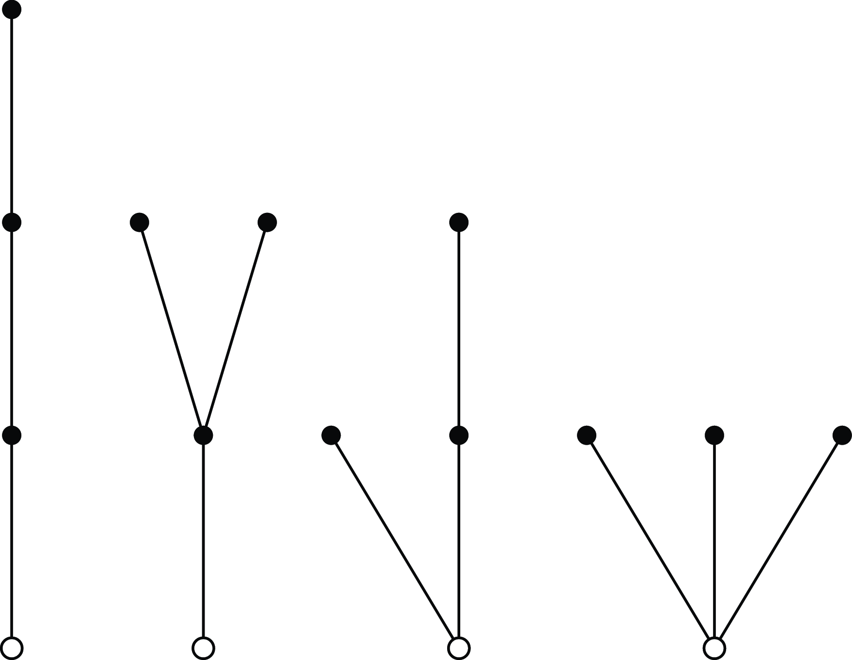
. The reason for the name ‘diamond area’ is that
$1/2$
. The reason for the name ‘diamond area’ is that $\sigma (X)$
is the signed area under the walk that lies outside a rotated checkerboard of diamonds, as in Figure 2.
$\sigma (X)$
is the signed area under the walk that lies outside a rotated checkerboard of diamonds, as in Figure 2.
A bridge $B$
with diamond area
$B$
with diamond area $\sigma (B)=2$
, which equals the signed area enclosed by
$\sigma (B)=2$
, which equals the signed area enclosed by $B$
and the
$B$
and the $x$
-axis, minus the area in grey. In the figure, the rotated squares all represent area
$x$
-axis, minus the area in grey. In the figure, the rotated squares all represent area $1$
. We also depict its lazy version
$1$
. We also depict its lazy version $\Lambda (B)$
, whose regular integral equals
$\Lambda (B)$
, whose regular integral equals $\sigma (B)$
.
$\sigma (B)$
.

Figure 2 Long description
The image depicts a bridge labeled B with a diamond-shaped area, denoted as sigma(B), which equals the signed area enclosed by B and the x-axis, minus the grey area. The figure includes rotated squares, each representing an area of 1. Additionally, the lazy version of the bridge, labeled Lambda(B), is shown, with its regular integral equaling sigma(B).
For walks $X=(X_0,X_1,\ldots )$
, we let
$X=(X_0,X_1,\ldots )$
, we let $X^{(k)}=(X_0,X_1,\ldots ,X_k)$
.
$X^{(k)}=(X_0,X_1,\ldots ,X_k)$
.
Definition 3.2. A bridge $B=(B_0,\ldots ,B_{2n})$
of length
$B=(B_0,\ldots ,B_{2n})$
of length $2n$
with increments
$2n$
with increments $\pm 1$
is graphical if
$\pm 1$
is graphical if $\sigma (B)=0$
and
$\sigma (B)=0$
and $\sigma _{2k}=\sigma (B^{(2k)})\ge 0$
, for all
$\sigma _{2k}=\sigma (B^{(2k)})\ge 0$
, for all $1\le k\lt n$
. A graphical bridge
$1\le k\lt n$
. A graphical bridge $B$
is irreducible if
$B$
is irreducible if $\sigma _{2k}\gt 0$
, for all
$\sigma _{2k}\gt 0$
, for all $1\le k\lt n$
. We let
$1\le k\lt n$
. We let $\mathcal{B}_n$
be the number of graphical bridges of length
$\mathcal{B}_n$
be the number of graphical bridges of length $2n$
. See Figure
3
.
$2n$
. See Figure
3
.
There are $\mathcal{B}_5=38$
graphical bridges of length
$\mathcal{B}_5=38$
graphical bridges of length $10$
. Of these, 32 stay within the string of grey diamonds centred along the
$10$
. Of these, 32 stay within the string of grey diamonds centred along the $x$
-axis. The other 6 are depicted above. The top two are irreducible. All others have two irreducible parts. Irreducible parts are separated by solid dots.
$x$
-axis. The other 6 are depicted above. The top two are irreducible. All others have two irreducible parts. Irreducible parts are separated by solid dots.

Figure 3 Long description
The image shows six graphical bridges of length 10 on a diamond grid. The bridges are represented by black lines connecting red and blue squares. The top two bridges are irreducible, while the others have two irreducible parts separated by solid dots. The bridges are set against a background of grey diamonds centered along the x-axis.
3.1 Relation to
$\rho$

Recall that $\rho$
is defined, in Section 1.1 above, in terms of a lazy random walk. We can rephrase
$\rho$
is defined, in Section 1.1 above, in terms of a lazy random walk. We can rephrase $\rho$
in terms of a standard, simple symmetric random walk
$\rho$
in terms of a standard, simple symmetric random walk $(X_n)$
with
$(X_n)$
with $\pm 1$
increments, started from
$\pm 1$
increments, started from $X_0=0$
, using its diamond area. Specifically, let
$X_0=0$
, using its diamond area. Specifically, let $\sigma _{2k}=\sigma (X^{(2k)})$
denote the diamond area accumulated after
$\sigma _{2k}=\sigma (X^{(2k)})$
denote the diamond area accumulated after $2k$
steps. Since, as discussed above, the diamond area of
$2k$
steps. Since, as discussed above, the diamond area of $X$
is the usual area of its lazy version
$X$
is the usual area of its lazy version $\Lambda (X)$
, it follows that
$\Lambda (X)$
, it follows that
 \begin{equation*} \rho =\textbf {P}(\sigma _{2\kappa }=0), \quad \quad \quad \kappa =\inf \{k\ge 1\,:\,X_{2k}=0,\: \sigma _{2k}\le 0\}. \end{equation*}
To see how $\rho$
relates to our problem, we observe that a bridge
$\rho$
relates to our problem, we observe that a bridge $B=(B_0,\ldots ,B_{2n})$
(with
$B=(B_0,\ldots ,B_{2n})$
(with $\pm 1$
increments) is graphical if and only if
$\pm 1$
increments) is graphical if and only if $\sigma (B)=0$
and
$\sigma (B)=0$
and $\sigma _{2k}=\sigma (B^{(2k)})\ge 0$
, for all times
$\sigma _{2k}=\sigma (B^{(2k)})\ge 0$
, for all times $2k$
for which
$2k$
for which $B_{2k}=0$
, since
$B_{2k}=0$
, since $\sigma$
is monotone between such diagnostic times. Then, roughly speaking,
$\sigma$
is monotone between such diagnostic times. Then, roughly speaking, $\rho$
is the probability that, the first time a random walk trajectory is in danger of not satisfying
$\rho$
is the probability that, the first time a random walk trajectory is in danger of not satisfying $\sigma _{2k}\ge 0$
, at such a diagnostic time
$\sigma _{2k}\ge 0$
, at such a diagnostic time $2k$
, the condition is in fact satisfied with equality
$2k$
, the condition is in fact satisfied with equality $\sigma _{2k}=0$
.
$\sigma _{2k}=0$
.
Consider now a random walk $X=(X_0,X_1,\ldots )$
. If
$X=(X_0,X_1,\ldots )$
. If $X_{2k}=\sigma _{2k}=0$
at the first diagnostic time
$X_{2k}=\sigma _{2k}=0$
at the first diagnostic time $2k\lt 2n$
, then
$2k\lt 2n$
, then $(X_0,\ldots ,X_{2n})$
is a graphical bridge if and only if
$(X_0,\ldots ,X_{2n})$
is a graphical bridge if and only if $(X_{2k},\ldots ,X_{2n})$
is a graphical bridge. Therefore, times at which
$(X_{2k},\ldots ,X_{2n})$
is a graphical bridge. Therefore, times at which $X_{2k}=\sigma _{2k}=0$
are of crucial importance, as they decompose a graphical bridge into its irreducible parts and correspond to renewal times in the analysis.
$X_{2k}=\sigma _{2k}=0$
are of crucial importance, as they decompose a graphical bridge into its irreducible parts and correspond to renewal times in the analysis.
Remark 3.1. As mentioned at the end of Section 2.3 above, the probability $\rho$
is only related to graphical bridges. Indeed, this can be seen directly from the definition of
$\rho$
is only related to graphical bridges. Indeed, this can be seen directly from the definition of $\rho$
in (5) above, since
$\rho$
in (5) above, since $\rho$
is the probability that, at time
$\rho$
is the probability that, at time $\tau$
, the walk
$\tau$
, the walk $Y=(Y_k,0\le k\le \tau )$
is the lazy version
$Y=(Y_k,0\le k\le \tau )$
is the lazy version $Y=\Lambda (B)$
of a graphical bridge
$Y=\Lambda (B)$
of a graphical bridge $B=(B_0,\ldots ,B_{2\tau })$
of length
$B=(B_0,\ldots ,B_{2\tau })$
of length $2\tau$
.
$2\tau$
.
Definition 3.3. We let $\mathcal{I}_n$
denote the number of irreducible parts in a uniformly random graphical bridge of length
$\mathcal{I}_n$
denote the number of irreducible parts in a uniformly random graphical bridge of length $2n$
.
$2n$
.
The following fact will play a central role in our arguments.
Lemma 3.1. We have that
 \begin{equation} \mathcal{I}_n\overset {d}{\to }1+\mathcal{X}, \end{equation}
where $\mathcal{X}$
is a negative binomial with parameters
$\mathcal{X}$
is a negative binomial with parameters $r=2$
and
$r=2$
and $p=1-\rho$
.
$p=1-\rho$
.
This result follows by (the proof of) [Reference Donderwinkel and Kolesnik5, Proposition 21]. The appearance of the negative binomial random variable can, intuitively, be explained as follows: with high probability, renewal times occur only very close to the start and end of the bridge. Moreover, the number of renewal times on either side are approximately geometric and independent.
3.2 Calculating
$\boldsymbol{\rho}$

We observed that a graphical bridge can be decomposed into a series of irreducible parts, and so $(\mathcal{B}_n,n\ge 0)$
is a renewal sequence. As discussed in Section 2, this means that the generating function
$(\mathcal{B}_n,n\ge 0)$
is a renewal sequence. As discussed in Section 2, this means that the generating function $\mathcal{B}(x)=\sum _n \mathcal{B}_nx^n$
can be expressed as
$\mathcal{B}(x)=\sum _n \mathcal{B}_nx^n$
can be expressed as
 \begin{equation*} \mathcal{B}(x)=\frac {1}{1-\mathcal{B}^{(1)}(x)}, \end{equation*}
where $\mathcal{B}^{(1)}(x)=\sum _n \mathcal{B}_n^{(1)}x^n$
is the generating function for the number
$\mathcal{B}^{(1)}(x)=\sum _n \mathcal{B}_n^{(1)}x^n$
is the generating function for the number $\mathcal{B}_n^{(1)}$
of irreducible graphical bridges of length
$\mathcal{B}_n^{(1)}$
of irreducible graphical bridges of length $2n$
.
$2n$
.
Therefore, by Lemma2.1(2), we have
 \begin{equation} \frac {\mathcal{B}_n^*}{n\mathcal{B}_n} =\textbf {E}\left [\frac {1}{\mathcal{I}_n}\right ]. \end{equation}
Note that $I_n\le 1$
, and so
$I_n\le 1$
, and so $1/I_n$
is uniformly integrable. Therefore, combining (15) and (16), we find that
$1/I_n$
is uniformly integrable. Therefore, combining (15) and (16), we find that
 \begin{equation} \frac {\mathcal{B}^*_n}{n\mathcal{B}_n}\to 1-\rho . \end{equation}
Hence, in proving Theorem1.2, the following is key.
Proposition 3.2.
We have that $\mathcal{B}^*_n=2 \mathcal{T}_n$
.
$\mathcal{B}^*_n=2 \mathcal{T}_n$
.
We prove Proposition3.2 in the next two sections. For now, let us note that our main result follows.
Proof of Theorem 1.2. By (1) and Proposition3.2,
 \begin{equation*} \frac {\mathcal{B}^*_n}{4^n} \sim \frac {1}{n4^n}\binom{2n}{n} \sim \frac {1}{\sqrt {\pi }n^{3/2}} \end{equation*}
is regularly varying with index $\gamma =-3/2$
. Therefore, by (9),
$\gamma =-3/2$
. Therefore, by (9),
 \begin{align} \frac {\mathcal{B}^*_n}{n\mathcal{B}_n} \to \exp\!(\!-2\omega ). \end{align}
Combining (17) and (18), we find that $\rho =1-\exp\!(\!-2\omega )$
, as claimed.
$\rho =1-\exp\!(\!-2\omega )$
, as claimed.
4. Combinatorial lemmas
In this section, we prove two combinatorial lemmas, showing that $2\mathcal{T}_n$
can be described in terms of areas
$2\mathcal{T}_n$
can be described in terms of areas $\alpha$
below lattice paths
$\alpha$
below lattice paths $L$
and diamond areas
$L$
and diamond areas $\sigma$
under bridges
$\sigma$
under bridges $B$
.
$B$
.
4.1 Lattice paths
Suppose that $L$
is an
$L$
is an $\uparrow ,\rightarrow$
lattice path from
$\uparrow ,\rightarrow$
lattice path from $(a_1,b_1)$
to
$(a_1,b_1)$
to $(a_2,b_2)$
, for some integers
$(a_2,b_2)$
, for some integers $a_1\le a_2$
and
$a_1\le a_2$
and $b_1\le b_2$
. We let
$b_1\le b_2$
. We let $\alpha (L)$
denote the area of the region between
$\alpha (L)$
denote the area of the region between $L$
and the lines
$L$
and the lines $x=a_2$
and
$x=a_2$
and $y=b_1$
.
$y=b_1$
.
Definition 4.1. We let $\mathcal{N}_n$
be the number of lattice paths
$\mathcal{N}_n$
be the number of lattice paths $L$
from
$L$
from $(0,0)$
to
$(0,0)$
to $(n,n)$
such that
$(n,n)$
such that $\alpha (L)\equiv 0$
mod
$\alpha (L)\equiv 0$
mod $n$
.
$n$
.
To see the relationship between $\mathcal{N}_n$
and
$\mathcal{N}_n$
and $\mathcal{T}_n$
, first note that the area of a lattice path
$\mathcal{T}_n$
, first note that the area of a lattice path $L$
from
$L$
from $(0,0)$
to
$(0,0)$
to $(n,n)$
is
$(n,n)$
is
 \begin{equation} \alpha (L)=\sum _i u_i, \end{equation}
summing over the sequence $u_1\le \cdots \le u_n$
, where
$u_1\le \cdots \le u_n$
, where $u_i$
is the number of
$u_i$
is the number of $\uparrow$
steps before the
$\uparrow$
steps before the $i$
th
$i$
th $\rightarrow$
step of
$\rightarrow$
step of $L$
. In other words, if we picture
$L$
. In other words, if we picture $L$
as a bar graph, then the
$L$
as a bar graph, then the $u_i$
are the heights of the bars. Hence,
$u_i$
are the heights of the bars. Hence, $\mathcal{N}_n$
is the number of submultisets of
$\mathcal{N}_n$
is the number of submultisets of $\{0,1,\ldots ,n\}$
of size
$\{0,1,\ldots ,n\}$
of size $n$
that sum to
$n$
that sum to $0$
mod
$0$
mod $n$
. On the other hand, recall that, as was already mentioned above,
$n$
. On the other hand, recall that, as was already mentioned above, $\mathcal{T}_n$
can be counted using a formula by von Sterneck.
$\mathcal{T}_n$
can be counted using a formula by von Sterneck.
Lemma 4.1 (von Sterneck [Reference Bachmann1, Reference Ramanathan16]). Let $\mathcal{S}_n$
be the number of submultisets
$\mathcal{S}_n$
be the number of submultisets $\{0,1,\ldots ,n-1\}$
of size
$\{0,1,\ldots ,n-1\}$
of size $n$
that sum to
$n$
that sum to $0$
mod
$0$
mod $n$
. Then
$n$
. Then $\mathcal{S}_n=\mathcal{T}_n$
.
$\mathcal{S}_n=\mathcal{T}_n$
.
Using these observations, we show the following.
Lemma 4.2.
We have that $\mathcal{N}_n = 2\mathcal{T}_n$
.
$\mathcal{N}_n = 2\mathcal{T}_n$
.
Proof.
Note that Lemma4.1 allows us to instead prove that $\mathcal{N}_n = 2\mathcal{S}_n$
. To this end, we first claim that
$\mathcal{N}_n = 2\mathcal{S}_n$
. To this end, we first claim that $\mathcal{S}_n$
is the number of
$\mathcal{S}_n$
is the number of $\uparrow ,\rightarrow$
lattice paths
$\uparrow ,\rightarrow$
lattice paths $L$
from
$L$
from $(0,0)$
to
$(0,0)$
to $(n,n-1)$
with
$(n,n-1)$
with $\alpha (L)\equiv 0$
mod
$\alpha (L)\equiv 0$
mod $n$
. Indeed, submultisets
$n$
. Indeed, submultisets $0\le u_1\le \cdots \le u_n\le n-1$
correspond to such
$0\le u_1\le \cdots \le u_n\le n-1$
correspond to such $L$
with
$L$
with $\rightarrow$
steps at heights
$\rightarrow$
steps at heights $u_i$
, and so
$u_i$
, and so $\alpha (L)=\sum _i u_i\equiv 0$
mod
$\alpha (L)=\sum _i u_i\equiv 0$
mod $n$
. Next, let
$n$
. Next, let $\mathcal{L}_n^\uparrow$
(resp.
$\mathcal{L}_n^\uparrow$
(resp. $\mathcal{L}_n^\rightarrow$
) be the number of lattice paths
$\mathcal{L}_n^\rightarrow$
) be the number of lattice paths $L$
from
$L$
from $(0,0)$
to
$(0,0)$
to $(n,n)$
such that
$(n,n)$
such that $\alpha (L)\equiv 0$
mod
$\alpha (L)\equiv 0$
mod $n$
, ending with an
$n$
, ending with an $\uparrow$
(resp.
$\uparrow$
(resp. $\rightarrow$
) step. Then
$\rightarrow$
) step. Then $\mathcal{N}_n=\mathcal{L}_n^\uparrow +\mathcal{L}_n^\rightarrow$
. To conclude, we show that
$\mathcal{N}_n=\mathcal{L}_n^\uparrow +\mathcal{L}_n^\rightarrow$
. To conclude, we show that $\mathcal{L}_n^\uparrow =\mathcal{L}_n^\rightarrow =\mathcal{S}_n$
. Indeed,
$\mathcal{L}_n^\uparrow =\mathcal{L}_n^\rightarrow =\mathcal{S}_n$
. Indeed, $\mathcal{L}_n^\uparrow =\mathcal{L}_n^\rightarrow$
follows by symmetry, reflecting over
$\mathcal{L}_n^\uparrow =\mathcal{L}_n^\rightarrow$
follows by symmetry, reflecting over $x=y$
, and observing that divisibility by
$x=y$
, and observing that divisibility by $n$
of the enclosed area is invariant under this reflection. Finally,
$n$
of the enclosed area is invariant under this reflection. Finally, $\mathcal{L}_n^\uparrow =\mathcal{S}_n$
, since if
$\mathcal{L}_n^\uparrow =\mathcal{S}_n$
, since if $L$
from
$L$
from $(0,0)$
to
$(0,0)$
to $(n,n)$
has last step
$(n,n)$
has last step $\uparrow$
, then removing this step yields a corresponding
$\uparrow$
, then removing this step yields a corresponding $L'$
from
$L'$
from $(0,0)$
to
$(0,0)$
to $(n,n-1)$
with the same area as
$(n,n-1)$
with the same area as $L$
.
$L$
.
4.2 Bridges
Next, we connect $\mathcal{N}_n$
to bridges.
$\mathcal{N}_n$
to bridges.
Definition 4.2. We let $\mathcal{N}_n'$
denote the number of bridges
$\mathcal{N}_n'$
denote the number of bridges $B$
of length
$B$
of length $2n$
, with diamond area
$2n$
, with diamond area $\sigma (B)\equiv 0$
mod
$\sigma (B)\equiv 0$
mod $n$
.
$n$
.
Lemma 4.3.
We have that $\mathcal{N}_n = \mathcal{N}_n'$
.
$\mathcal{N}_n = \mathcal{N}_n'$
.
Proof.
To obtain a correspondence between bridges $B=(B_0,\ldots ,B_{2n})$
of length
$B=(B_0,\ldots ,B_{2n})$
of length $2n$
such that
$2n$
such that $\sigma (B)\equiv 0$
mod
$\sigma (B)\equiv 0$
mod $n$
and lattice paths
$n$
and lattice paths $L$
from
$L$
from $(0,0)$
to
$(0,0)$
to $(n,n)$
with
$(n,n)$
with $a(L)\equiv 0$
mod
$a(L)\equiv 0$
mod $n$
, we proceed as follows.
$n$
, we proceed as follows.
First, let $\Delta _i = B_i-B_{i-1}$
be the
$\Delta _i = B_i-B_{i-1}$
be the $i$
th increment of
$i$
th increment of $B$
. For
$B$
. For $1\le k\le n$
, put
$1\le k\le n$
, put
 \begin{equation*} B^{\mathrm{odd}}_k=\sum _{i=1}^k \Delta _{2i-1}, \quad \quad B^{\mathrm{even}}_k=\sum _{i=1}^k \Delta _{2i}, \end{equation*}
so that $B^{\mathrm{odd}}=(B^{\mathrm{odd}}_1,\ldots ,B^{\mathrm{odd}}_n)$
and
$B^{\mathrm{odd}}=(B^{\mathrm{odd}}_1,\ldots ,B^{\mathrm{odd}}_n)$
and $B^{\mathrm{even}}=(B^{\mathrm{even}}_1,\ldots ,B^{\mathrm{even}}_n)$
are the walks with the odd and even increments of
$B^{\mathrm{even}}=(B^{\mathrm{even}}_1,\ldots ,B^{\mathrm{even}}_n)$
are the walks with the odd and even increments of $B$
, respectively.
$B$
, respectively.
Next, rotate $B^{\mathrm{odd}}$
counterclockwise by
$B^{\mathrm{odd}}$
counterclockwise by $\pi /4$
to obtain a lattice path
$\pi /4$
to obtain a lattice path $L_1$
from
$L_1$
from $(0,0)$
to
$(0,0)$
to $(n-\ell ,\ell )$
for some
$(n-\ell ,\ell )$
for some $\ell$
(since
$\ell$
(since $B^{\mathrm{odd}}$
has
$B^{\mathrm{odd}}$
has $n$
steps). Likewise, rotate
$n$
steps). Likewise, rotate $B^{\mathrm{even}}$
counterclockwise by
$B^{\mathrm{even}}$
counterclockwise by $\pi /4$
to obtain a lattice walk
$\pi /4$
to obtain a lattice walk $L_2$
from
$L_2$
from $(n-\ell ,\ell )$
to
$(n-\ell ,\ell )$
to $(n,n)$
(since
$(n,n)$
(since $B$
is a bridge). Let
$B$
is a bridge). Let $L$
be the concatenation of
$L$
be the concatenation of $L_1$
and
$L_1$
and $L_2$
. This procedure is depicted in Figure 4.
$L_2$
. This procedure is depicted in Figure 4.
The bijection in Lemma4.3.

Figure 4 Long description
A flowchart illustrating a bijection in Lemma 4.3. The diagram features two main paths: one zigzagging upwards from the origin (0,0) to the point (2n,0) labeled B, and another path moving right and upwards to the point (n,n). The paths are marked with arrows indicating direction. Key points are labeled, such as (0,0), (2n,0), (n,n), and (n-ℓ,ℓ). The paths are divided into segments labeled α(L1), α(L2), and ℓ², with L representing a horizontal segment. The diagram visually represents the relationship and transformation between different sequences in a graphical context.
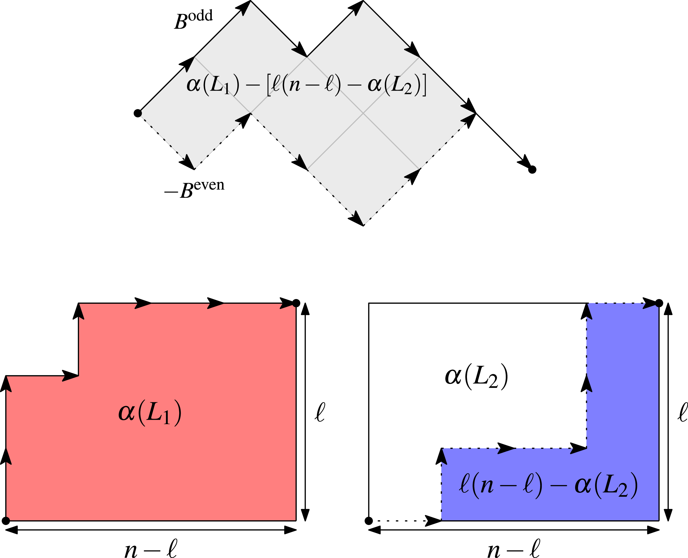
Calculating areas in Lemma4.3.

Figure 5 Long description
The diagram consists of three main parts. The top part shows a diamond-shaped figure with arrows indicating directions and labeled with mathematical expressions involving alpha, B odd, and B even. The bottom left part depicts a red square with a notch, labeled with alpha L1 and dimensions n minus l by l. The bottom right part shows a white square with blue regions, labeled with alpha L2 and l times n minus l minus alpha L2, with dimensions n minus l by l. Arrows indicate the flow and relationships between the different sections.
Geometric considerations (see Figure 5) imply that
 \begin{equation*} \alpha (L) =\alpha (L_1)+\alpha (L_2)+\ell ^2. \end{equation*}
Furthermore, observe that, by definition,
 \begin{equation*} \sigma (B) =\frac {1}{2}\sum _{i=1}^n \sum _{j=1}^i \left ( \Delta _{2j-1} + \Delta _{2j}\right ) =\frac {1}{2}\sum _{k=1}^n (B^{\mathrm{odd}}_k+B^{\mathrm{even}}_k), \end{equation*}
which equals the signed area enclosed by $B^{\mathrm{odd}}$
and
$B^{\mathrm{odd}}$
and $-B^{\mathrm{even}}$
, as depicted in Figure 5. Therefore, it can be seen that
$-B^{\mathrm{even}}$
, as depicted in Figure 5. Therefore, it can be seen that
 \begin{equation*} \sigma (B) =\alpha (L_1)-[\ell (n-\ell )-\alpha (L_2)] =\alpha (L)-\ell n. \end{equation*}
Since $\alpha (L)\equiv \sigma (B)$
mod
$\alpha (L)\equiv \sigma (B)$
mod $n$
, this completes the proof.
$n$
, this completes the proof.
5. The Lévy–Khintchine transform
We are now in a position to prove our key result Proposition3.2, which identifies $\mathcal{B}_n^*= 2\mathcal{T}_n$
as the Lévy–Khintchine transform of
$\mathcal{B}_n^*= 2\mathcal{T}_n$
as the Lévy–Khintchine transform of $\mathcal{B}_n$
.
$\mathcal{B}_n$
.
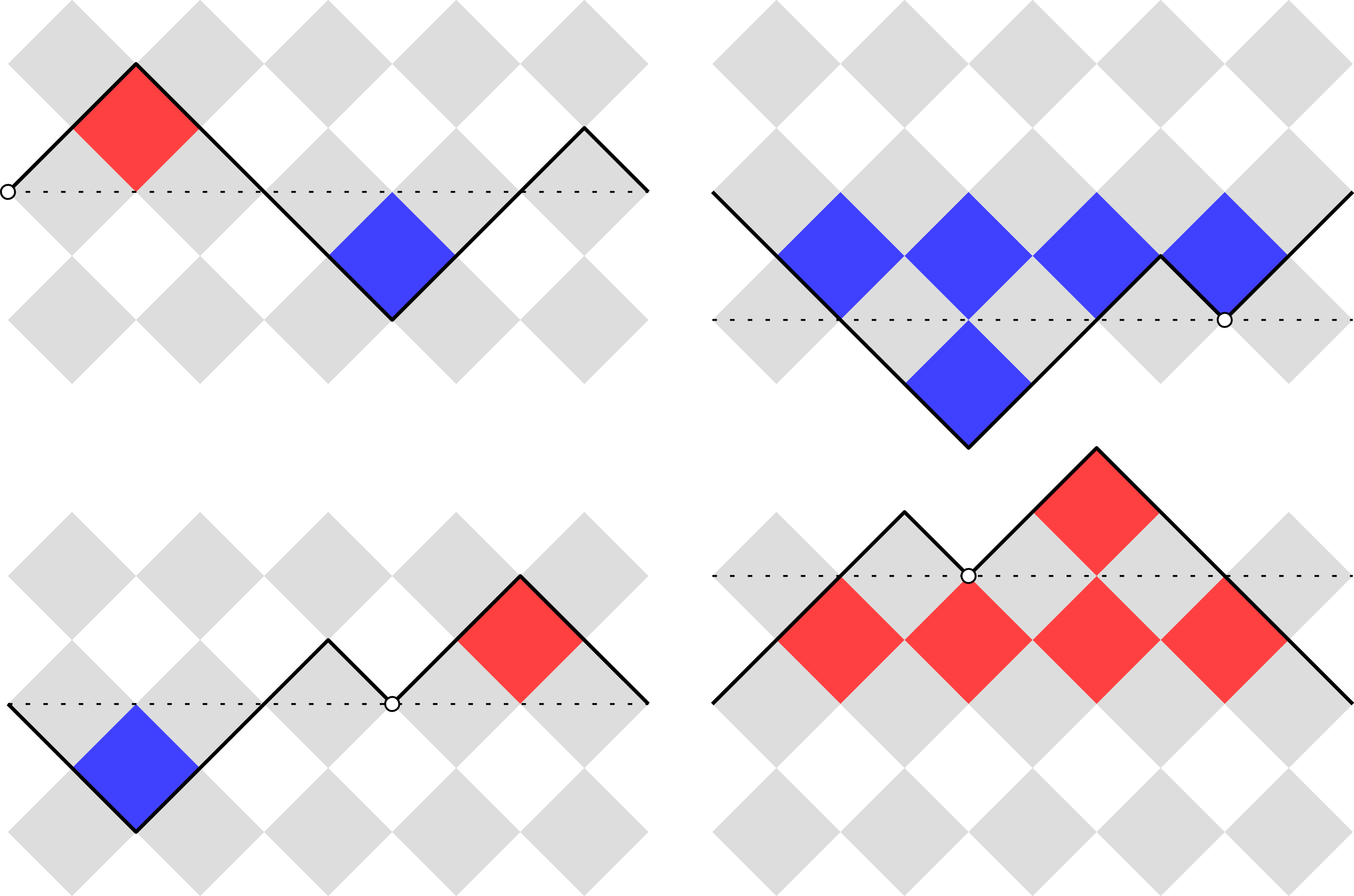
A graphical bridge $B$
(top left) of length 10, with first irreducible part of length 8. The bridge
$B$
(top left) of length 10, with first irreducible part of length 8. The bridge $B$
is
$B$
is $\phi (B,0)$
. Its other shifts
$\phi (B,0)$
. Its other shifts $\phi (B,i)$
, for
$\phi (B,i)$
, for $1\le i\lt 4$
, are also depicted. All bridges have diamond area divisible by 5. To find the inverse mapping
$1\le i\lt 4$
, are also depicted. All bridges have diamond area divisible by 5. To find the inverse mapping $\phi ^{-1}$
, we shift the
$\phi ^{-1}$
, we shift the $x$
-axis (see dotted line) by some factor of 2 so that the diamond area is equal to 0, and then find the rightmost point (open dot) that starts a graphical sequence. Such a point exists by Raney’s lemma.
$x$
-axis (see dotted line) by some factor of 2 so that the diamond area is equal to 0, and then find the rightmost point (open dot) that starts a graphical sequence. Such a point exists by Raney’s lemma.

Figure 6 Long description
The image depicts a graphical bridge labeled B with a total length of 10 units, where the first irreducible part has a length of 8 units. The bridge B is represented as phi(B,0). The image also shows other shifts of the bridge, denoted as phi(B,i) for values of i ranging from 1 to less than 4. All bridges depicted have diamond areas that are divisible by 5. To find the inverse mapping phi inverse, the x-axis is shifted by a factor of 2 so that the diamond area equals 0, and then the rightmost point that starts a graphical sequence is identified. This point is marked with an open dot and its existence is guaranteed by Raney's lemma.
Proof of Proposition
3.2
. As discussed, $(\mathcal{B}_n,n\ge 0)$
is a renewal sequence, and so
$(\mathcal{B}_n,n\ge 0)$
is a renewal sequence, and so $\mathcal{B}_n^*$
can be described in terms of Lemma2.1(1). Combining this with our combinatorial results Lemmas4.2 and 4.3 above, it follows that, to show that
$\mathcal{B}_n^*$
can be described in terms of Lemma2.1(1). Combining this with our combinatorial results Lemmas4.2 and 4.3 above, it follows that, to show that $\mathcal{B}_n^*=2\mathcal{T}_n$
, it suffices to find a bijection:
$\mathcal{B}_n^*=2\mathcal{T}_n$
, it suffices to find a bijection:
-
• from the set of ordered pairs
$(B,i)$
, where
$B$
is a graphical bridge of length
$2n$
, whose first irreducible part is of length
$2\ell$
, and
$0\le i\lt \ell$
-
• to the set of bridges
$B'$
of length
$2n$
, with diamond area
$\sigma (B')\equiv 0$
mod
$n$
.


We claim that such a bijection can be constructed as follows: for each such pair $(B,i)$
, let
$(B,i)$
, let $\phi (B,i)$
be the bridge
$\phi (B,i)$
be the bridge $B'$
obtained from
$B'$
obtained from $B$
, via a cyclical shift to the right by
$B$
, via a cyclical shift to the right by $2i$
. Note that, geometrically,
$2i$
. Note that, geometrically, $B'$
can be obtained from
$B'$
can be obtained from $B$
by shifting the
$B$
by shifting the $x$
-axis up or down by some multiple of
$x$
-axis up or down by some multiple of $2$
and then starting the bridge from a particular intersection point of the new
$2$
and then starting the bridge from a particular intersection point of the new $x$
-axis and the bridge
$x$
-axis and the bridge $B$
. Only the former operation affects the total diamond area. In fact, by (14), it can be seen that such a shift changes the area by a multiple of
$B$
. Only the former operation affects the total diamond area. In fact, by (14), it can be seen that such a shift changes the area by a multiple of $n$
. Since
$n$
. Since $\sigma (B)=0$
, it follows, again by (14), that
$\sigma (B)=0$
, it follows, again by (14), that $\sigma (B')\equiv 0$
mod
$\sigma (B')\equiv 0$
mod $n$
. See Figure 6.
$n$
. See Figure 6.
On the other hand, for any $B'$
with
$B'$
with $\sigma (B')\equiv 0$
mod
$\sigma (B')\equiv 0$
mod $n$
, the inverse
$n$
, the inverse $\phi ^{-1}(B')$
is found as follows. Select the unique shift of the
$\phi ^{-1}(B')$
is found as follows. Select the unique shift of the $x$
-axis for which the diamond area becomes 0, and then choose the rightmost starting point
$x$
-axis for which the diamond area becomes 0, and then choose the rightmost starting point $2n-2i$
for which the resulting bridge
$2n-2i$
for which the resulting bridge $B$
is graphical; then
$B$
is graphical; then $\phi ^{-1}(B')=(B,i)$
. Such a point exists by Raney’s lemmaFootnote
1
[Reference Raney17], and by choosing
$\phi ^{-1}(B')=(B,i)$
. Such a point exists by Raney’s lemmaFootnote
1
[Reference Raney17], and by choosing $i$
minimal we ensure that
$i$
minimal we ensure that $2i$
is smaller than the length of the first irreducible part of
$2i$
is smaller than the length of the first irreducible part of $B$
.
$B$
.
Acknowledgments
We thank the referees whose comments helped improve the presentation of this article. MB is supported by a Clarendon Fund Scholarship and a Keble Sloane-Robinson Graduate Scholarship. SD acknowledges the financial support of the CogniGron research center and the Ubbo Emmius Funds (Univ. of Groningen). Her research was also supported by the Marie Skłodowska-Curie grant GraPhTra (Universality in phase transitions in random graphs), grant agreement ID 101211705. BK was partially supported by a Florence Nightingale Bicentennial Fellowship (Oxford Statistics) and a Senior Demyship (Magdalen College).


 T3=4
T3=4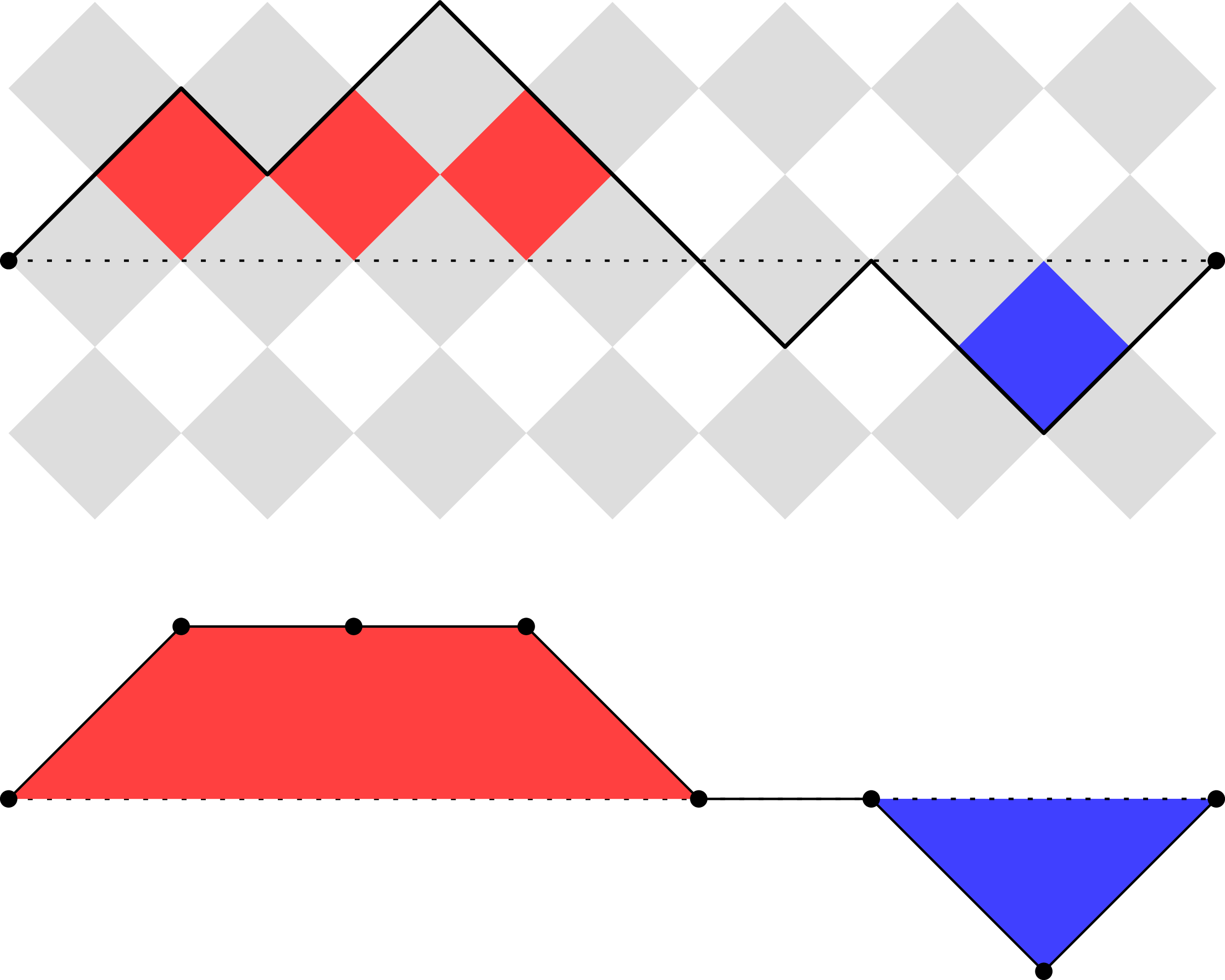
 B
B σ(B)=2
 B
B x
x 1
1 Λ(B)
Λ(B) σ(B)
σ(B)
 B5=38
B5=38 10
10 x
x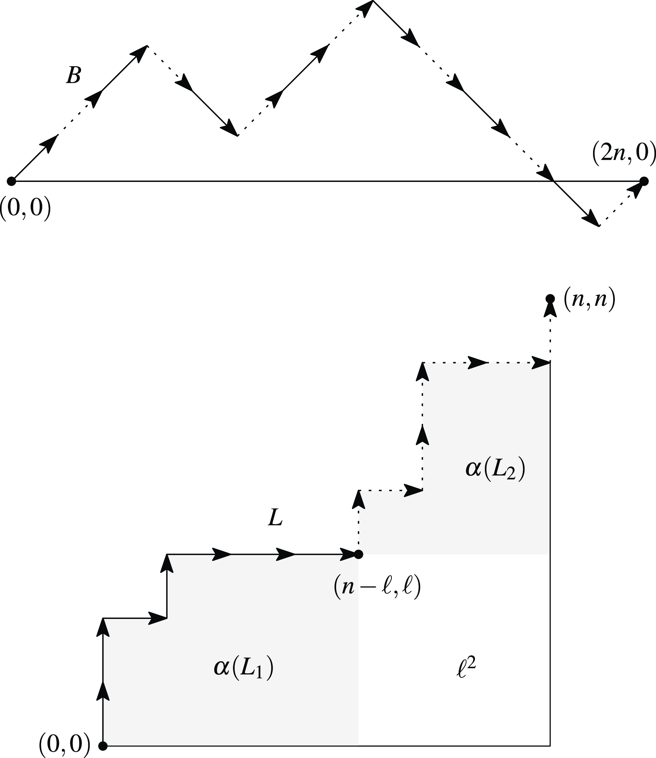
 B
B B
B ϕ(B,0)
 ϕ(B,i)
 1≤i<4
1≤i<4 ϕ−1
ϕ−1 x
x
 Open access