


1. Introduction
1.1 Overview
In his seminal work [Reference RouquierRou08], Rouquier introduced a notion of dimension for triangulated categories. A sketch of the definition may be given as follows: if  $\mathcal {T}$ is a triangulated category and $G$ is a (split) generator, then $G$ is said to generate $\mathcal {T}$ in time $t$ if every object of $\mathcal {T}$ can be built from $G$ by taking finite direct sums, shifts, summands, and at most $t$ cones. The Rouquier dimension of $\mathcal {T}$ is, by definition, the minimal generation time over all generators of $\mathcal {T}$. (If $\mathcal {T}=0$, then we define the dimension to be $-1$.)
In symplectic topology, an important class of triangulated categories are derived Fukaya categories in their various guises. We are mainly interested in wrapped Fukaya categories of Liouville manifolds. More precisely, given a Liouville manifold  $(X, \lambda )$, its wrapped Fukaya category $\mathcal {W}(X)$ is an $A_\infty$ category and, as such, it canonically determines a triangulated category $H^0(\operatorname {Perf} \mathcal {W}(X))$. The Rouquier dimension of this triangulated category is a numerical invariant of $(X, \lambda )$, which is the focus of this paper.
Our applications are twofold: first, to a problem in algebraic geometry; second, to quantitative questions in symplectic topology. We discuss each of these two classes of applications in turn in the remainder of this introduction.
1.2 An application of symplectic topology to algebraic geometry
1.2.1 Motivation
In classical algebraic geometry, one is typically interested in spaces (varieties, schemes, stacks, etc.) which are locally modeled on the spectrum of a commutative ring. According to the philosophy of non-commutative geometry, it is often profitable to regard  $A_\infty$ categories as ‘non-commutative’ spaces. One can then attempt to generalize classical algebraic geometry to the setting of $A_\infty$ category theory.
For example, there are standard notions smoothness, properness, dimension, etc. in classical algebraic geometry. It turns out that there also exist non-commutative analogs of some of these notions. Namely, an  $A_\infty$ category is defined to be smooth if its diagonal bimodule is perfect; it is defined to be proper if its diagonal bimodule is proper.Footnote 1 The dimension of an $A_\infty$ category is simply its Rouquier dimension.Footnote 2
If  $Y$ is an ordinary algebraic variety, then one can associate to it the $A_\infty$ category $D^b\operatorname {Coh}(Y)$. One typically regards $D^b\operatorname {Coh}(Y)$ as the non-commutative partner of the classical object $Y$. It is then natural to ask: do the non-commutative notions of smoothness, properness, and dimension coincide with their classical counterparts?
As one might hope, it is known that  $D^b\operatorname {Coh}(Y)$ is smooth and proper if and only if $Y$ is smooth and proper in the classical sense. Concerning dimension, there is the following well-known conjecture of Orlov.
Conjecture 1.1 (Orlov [Reference OrlovOrl09a, Conjecture 10])
Let  $Y$ be a smooth quasi-projective scheme of dimension $n$. Then
 \begin{equation} \operatorname{Rdim}D^{b} \operatorname{Coh}(Y) = n. \end{equation}
 The assumption that  $Y$ is smooth is necessary; see Example 2.17. Orlov's conjecture is, in general, wide open. It has only been established for the following rather restrictive classes of examples, thanks to the combined work of many authors (to the best of the authors’ knowledge, this list is exhaustive).
(i) Smooth affine varieties, projective spaces, and smooth projective quadrics [Reference RouquierRou08, Proposition 7.18, Examples 7.7, 7.8].
(ii) All smooth projective curves [Reference OrlovOrl09a, Theorem 6].
(iii) The following schemes defined over an algebraically closed field of characteristic $0$: del Pezzo surfaces with $\operatorname {rk} \operatorname {Pic}(Y) \leqslant 7$, Fano threefolds of type $V_5$ and $V_{22}$, toric surfaces with nef anti-canonical divisor, toric Deligne–Mumford stacks defined over $\mathbb {C}$ of dimension no more than $2$ or Picard number no more than $2$, Hirzebruch surfaces [Reference Ballard and FaveroBF12].
(iv) The product of varieties from (iii) [Reference YangYan16].
(v) The product of two Fermat elliptic curves with the Fermat
$K3$ surface [Reference Ballard, Favero and KatzarkovBFK14, Theorem 1.6].(vi) Smooth toric Fano varieties of dimension
$3$ or $4$ [Reference Ballard, Duncan and McFaddinBDM19, Propositions 2.15 and 2.16].(vii) Certain blow-ups of the projective space [Reference PirozhkovPir19, Theorem 4.1].
(viii) Some weak del Pezzo surfaces [Reference Elagin, Xu and ZhangEXZ21, Corollary 7.5].


We remark that Rouquier proved that, for smooth  $Y$,
$Y$,
 \begin{equation} n \leqslant \operatorname{Rdim}D^{b} \operatorname{Coh}(Y) \leqslant 2n, \end{equation}
so the content of Orlov's conjecture lies in improving the upper bound. See § 2.6 for further discussion and references.
1.2.2 Results
We introduce new methods from the flexible side of symplectic topology to study Orlov's conjecture. More precisely, we prove the following result.
Theorem 1.2 Suppose that  $Y$ is a variety over $\mathbb {C}$ of complex dimension $n$ which admits a homological mirror given by a polarizable Weinstein pair. Then $\operatorname {Rdim}D^b\operatorname {Coh}(Y)=n$ if $n \leqslant 3$. For $n \geqslant 4$, we have $\operatorname {Rdim}D^b\operatorname {Coh}(Y)\leqslant 2n -3$.
(A Weinstein pair  $(X, A)$ is said to be polarizable if $X$ admits a global Lagrangian plane field $\xi$.) Theorem 1.2 implies the following new cases of Orlov's conjecture.
Corollary 1.3 Conjecture 1.1 is true for all three-dimensional toric varieties over  $\mathbb {C}$ and the log Calabi–Yau surfaces in Example 4.20.
In fact, Theorem 1.2 shows that (1.1) holds for a large class of (possibly singular) schemes and stacks over  $\mathbb {C}$, see § 4.4 for the list. It also gives a new proof of some of the known cases of Orlov's conjecture listed above. Finally, Theorem 1.2 improves Rouquier's upper bound (1.2) for $\operatorname {Rdim}D^b\operatorname {Coh}(-)$ for many examples in dimensions $n \geqslant 4$ (including all smooth toric varieties and DM stacks).
1.2.3 Methods: symplectic flexibility
Although Orlov's conjecture is a problem in algebraic geometry, our proof of Theorem 1.2 is entirely symplectic. As mentioned in (1.2), it is already known that  $\operatorname {Rdim}D^b\operatorname {Coh}(Y) \geqslant n$. Hence, we only need to prove the claimed upper bounds. To do this, we apply homological mirror symmetry. This transforms Theorem 1.2 into a statement about the Rouquier dimension of wrapped Fukaya categories of Weinstein pairs; namely, it is enough to prove that the Rouquier dimension of a (polarizable) Weinstein pair of real dimension $2n$ is bounded above by $n$ when $n \leqslant 3$ and by $2n-3$ when $n \geqslant 4$. This is now purely a problem in symplectic topology which can be approached using symplectic tools.
According to the recent work of Ganatra, Pardon, and Shende [Reference Ganatra, Pardon and ShendeGPS22], wrapped Fukaya categories of Liouville manifolds satisfy ‘Weinstein sectorial descent’. Essentially, this means that if we (suitably) cover a Liouville manifold  $X$ by Weinstein sectors $\{ X_\alpha \}_{\alpha \in I}$, then $\mathcal {W}(X)$ can be expressed as the homotopy colimit of the wrapped Fukaya categories of the form $\mathcal {W}(\cap _{\alpha \in J} X_\alpha )$ (where $J$ ranges over all non-empty subsets of $I$ and the homotopy colimit is indexed by the obvious diagram of inclusions).
It is not hard to show that the Rouquier dimension of a homotopy colimit can be bounded from above by the Rouquier dimension of its individual pieces. This bound depends on (a) the ‘depth’ of the diagram (i.e. the longest chain of arrows) and (b) the Rouquier dimension of the individual pieces; see Lemma 2.15 for a precise statement. This suggests a possible strategy for upper bounding the Rouquier dimension of a Weinstein manifold: construct a sectorial cover of ‘small’ depth, such that each piece in the cover has ‘small’ Rouquier dimension.
Let us first implement this strategy in the special case where  $X=T^*M$, for $M$ a closed $n$-manifold. We construct a sectorial cover as follows. First, triangulate $M$. Then set $X_\alpha := T^*\operatorname {star}(v_\alpha )$ where $v_\alpha$ ranges over the vertices of the triangulation. Observe that the intersection of any collection of stars in a triangulation is either empty, or is the star of some higher-dimensional cell. From this, it follows that the cover has depth $n+1$. It also follows (after appropriate smoothing) that $\bigcap _{\alpha _1, \ldots, \alpha _n} T^*\operatorname {star}(v_{\alpha _i}) \simeq T^*D^n$ and, hence, the Rouquier dimension of the overlaps is zero. Plugging these numbers into Lemma 2.15, one finds that $\operatorname {Rdim} \mathcal {W}(T^*M) \leqslant n$. This upper bound is sharp in general.Footnote 3
We would like to extend this argument to an arbitrary Weinstein manifold  $X$. Unfortunately, the naive generalization does not work. If $X$ is an arbitrary Weinstein manifold, its skeleton may be a highly singular object. Even assuming the skeleton can be triangulated (which is not automatic), it is completely unclear how to control the Rouquier dimension of the resulting sectorial cover. It is also unclear how to convert a cover of the skeleton into a sectorial cover of its thickening (in the cotangent bundle case, there is a canonical Morse–Bott form which allows one to easily perform this conversion).
To overcome these difficulties, we take advantage of recent advances from the flexible side of symplectic geometry. Namely, the arborealization theorem of Álvarez-Gavela, Eliashberg, and Nadler [Reference Alvarez-Gavela, Eliashberg and NadlerAGEN21a, Reference Alvarez-Gavela, Eliashberg and NadlerAGEN21b, Reference Alvarez-Gavela, Eliashberg and NadlerAGEN20] provides an h-principle for simplifying the singularities of the skeleton. The upshot is that, under rather mild topological assumptions, one can homotope a Weinstein manifold so that the singularities of its skeleton are of ‘arboreal’ type. Such homotopies do not affect the wrapped Fukaya category.
Arboreal singularities are indexed by finite rooted trees. Morally, if  $\mathcal {S}_\sigma$ is a Liouville sector obtained by thickening an arboreal singularity $\sigma$, one expects that $\mathcal {W}(\mathcal {S}_\sigma )$ is Morita equivalent to $\operatorname {Rep}(T_\sigma )$, the derived representation category of the corresponding tree $T_\sigma$. Moreover, it is known that $\operatorname {Rdim} \operatorname {Rep}(T_\sigma )=0$ if $T_\sigma$ is of Dynkin type (i.e. the underlying graph is a Dynkin diagram) and $\operatorname {Rdim} \operatorname {Rep}(T_\sigma )=1$ otherwise. This suggests that sectorial thickenings of arboreal singularities are a good substitute for $T^*D^n$.
Arboreal skeleta admit a canonical stratification by ‘singularity order’. We prove in § 4.2 that this stratification is Whitney. By a well-known theorem of Goresky, any Whitney stratification can be refined to a (possibly non-Whitney) triangulation. This suggests the following updated strategy: given a (polarizable) Weinstein manifold  $X$ of dimension $2n$, apply a homotopy to make the skeleton arboreal. It therefore admits a triangulation. Now construct a sectorial cover by taking arboreal thickenings of the stars of the vertices, like for cotangent bundles.
Unfortunately, there are significant obstructions to making this strategy rigorous. To begin with, one would need to develop a good theory of arboreal sectors (which should be closed under intersections), as well as a procedure for constructing a ‘sectorial thickening’ of an arboreal singularity. Moreover, one would need a method for construct arboreal sectors from stars of (possibly non-Whitney) triangulations. Due to this difficulties, it is unclear to us whether the above strategy can feasibly be implemented in the framework of Fukaya categories.
Instead, we work in the framework of microlocal sheaf theory. The details of this approach are carried out in § 4. After reviewing some basic properties of microlocal sheaves, we study the stratified topology of arboreal skeleta, and use this to construct a suitable triangulation. We then carry through a microlocal sheaf analog of the above covering argument to obtain an upper bound on the Rouquier dimension of the category of microlocal sheaves. Finally, we apply the main result of [Reference Ganatra, Pardon and ShendeGPS20b] to pass back to wrapped Fukaya categories.
The precise upper bound which we obtain via this argument (and under the assumption that  $X$ is stably polarizable) is $\operatorname {Rdim} \mathcal {W}(X^{2n}) \leqslant n$ for $n \leqslant 3$, and $\operatorname {Rdim} \mathcal {W}(X^{2n}) \leqslant 2n-3$ for $n>3$. We know no counterexample to the inequality $\operatorname {Rdim} \mathcal {W}(X^{2n}) \leqslant n$ for arbitrary Weinstein manifolds.
1.2.4 A digression on motives
As a byproduct of our method, we derive some consequences for the structure of non-commutative motives on partially wrapped Fukaya categories. The notion of a non-commutative motive is was introduced by Tabuada [Reference TabuadaTab15] and is briefly summarized in § 4.5. To give an illustration, suppose that  $(X,A)$ is a polarizable Weinstein pair such that $\mathcal {W}(X,A)$ is proper (it is always smooth according to [Reference Ganatra, Pardon and ShendeGPS22, Corollary 1.19]). Then we find that:
(i)
$HH_\bullet (\mathcal {W}(X,A))$ is concentrated in degree zero;(ii)
$\operatorname {Perf} \mathcal {W}(X,A)$ satisfies the non-commutative Weil conjecture introduced by Tabuada (following proposals of Kontsevich) in [Reference TabuadaTab22].


Both of these statements follow from a more general result about non-commutative motives, which is itself an easy consequence of the arborealization method described previously. We refer the reader to § 4.5 for details.
1.3 Quantitative problems in symplectic topology
1.3.1 Motivation
As motivation for the geometrically inclined symplectic topologist, we state some quantitative questions of rather classical flavor.
Question 1.4 Let  $(X, \lambda )$ be a WeinsteinFootnote 4 manifold with skeleton ${\frak c}_X$. If $\phi : X \to X$ is a compactly supported Hamiltonian diffeomorphism, what is the minimal possible number of intersection points of $\phi ({\frak c}_X)$ with ${\frak c}_X$?
If  $(X, \lambda )=(T^*M, pdq)$ for a closed manifold $M$, then ${\frak c}_X= 0_M$ and Question 1.4 is classical. As is now well-known, it follows from the existence of Floer cohomology (or finite-dimensional analogs) that $|{\frak c}_X \cap \phi ({\frak c}_X)|$ is bounded from below by the sum of the Betti numbers of $M$.
$M$.
In general, however, the skeleton of a Weinstein manifold is a highly singular object for which there is no available notion of Floer cohomology (and it seems rather unlikely that such a notion exists). Note that even for the cotangent bundle of a closed manifold, equipped with a Weinstein structure homotopic to the standard Morse–Bott one, the skeleton is typically singular.
To the best of the authors’ knowledge, the only systematic result in the literature addressing Question 1.4 is the lower bound  $|{\frak c}_X \cap \phi ({\frak c}_X)| \geqslant 1$, which holds whenever the Rabinowitz–Floer homology $RFH(X)$ is non-zero [Reference Cieliebak and FrauenfelderCF09]. The nonvanishing of $RFH(-)$ for Weinstein manifolds is now known to be equivalent to the nonvanishing of $SH(-)$ and $\mathcal {W}(-)$; see [Reference RitterRit13, § 1.6].
Question 1.5 Let  $X$ be a Liouville manifold, considered up to homotopy. What is the minimal possible number of critical points of a Lefschetz fibration $f: X \to \mathbb {C}$ with Weinstein fibers?
Let us denote this number by  $\operatorname {Lef}_w(X) \in \mathbb {N} \cup \{\infty \}$. According to work of Giroux and Pardon [Reference Giroux and PardonGP17], any Weinstein manifold admits a Lefschetz fibration with Weinstein fibers, so $\operatorname {Lef}_w(X)<\infty$ if and only if $X$ is Weinstein (up to homotopy). It is also clear that $\operatorname {Lef}_w(X)=0$ if and only if $X$ is subcritical (by a result of Cieliebak [Reference CieliebakCie02], this means equivalently that $X$ admits a Weinstein presentation with only handles of index strictly less than the middle dimension, or that $X$ is Weinstein deformation equivalent to the product of a lower-dimensional Weinstein manifold with $\mathbb {C}$). For topological reasons, one has the lower bound $\operatorname {Lef}_w(X) \geqslant \operatorname {rk} H_n(X; \mathbb {Z})$ when $X$ has real dimension $2n$. These are the only lower bounds in the literature that we are aware of.
An analog of  $\operatorname {Lef}_w(X)$ in real Morse theory was considered by Abouzaid and Seidel [Reference Abouzaid and SeidelAbSe10b] under the name ‘complexity’. By definition, the complexity of a Weinstein manifold $X$, which we denote by $\operatorname {WMor}(X)$, is the minimal number of critical points of a Weinstein Morse function on $X$, where $X$ is considered up to Weinstein homotopy.Footnote 5 Surprisingly, Lazarev [Reference LazarevLaz20] showed that for Weinstein manifolds having non-zero middle homology, one has $\operatorname {WMor}(X)= \operatorname {Mor}(X)$, where $\operatorname {Mor}(X)$ denotes the minimal number of critical points of a smooth Morse function on $X$. Does a similar phenomenon hold for $\operatorname {Lef}_w(X)$?
1.3.2 Results
We give partial answers to the above questions. As we explain, our results appear to be the first to go beyond the basic flexible/rigid dichotomy.
We first consider Question 1.4. To this end, suppose that  $(X, \lambda )$ be a Weinstein manifold with properly embedded cocores (this is a generic condition). Let $R \subseteq SH^0(X)$ be a subalgebra which is of finite type over a field $k$, and suppose that there exists a (split-)generating Lagrangian $K \in \mathcal {W}(X)$ such that $HW^\bullet (K,K)$ is a Noetherian $R$-module, where $R$ acts via the closed–open string map.
Theorem 1.6 (= Proposition 6.9 + Theorem 5.2)
Under the above assumptions, if  $\phi : X \to X$ is a generic compactly supported Hamiltonian symplectomorphism, then
 \begin{equation} | {\frak c}_X \cap \phi({\frak c}_X) | \geqslant \dim_R HW^\bullet(K,K) +1. \end{equation}
 Here  $\dim _R (-)$ denotes the Krull dimension of an $R$-module. Both $\mathcal {W}(X)$ and $SH^{\bullet }(X)$ are defined over $k$ and are, say, $\mathbb {Z}/2$-graded. Here are some examples illustrating applications of Theorem 1.6.
Example 1.7 For  $(T^*S^n, \lambda )$, where $n \geqslant 2$ and $\lambda$ is homotopic to the standard Morse–Bott form $pdq$, we show that $\operatorname {Rdim} \mathcal {W}(T^*S^n)=1$ (say with $\mathbb {Z}/2$-gradings and $\mathbb {Q}$-coefficients) and, hence, $|{\frak c}_X \cap \phi ({\frak c}_X)| \geqslant 2$. This lower bound is of course sharp.
Example 1.8 Let  $G$ be a compact, simply connected Lie group. Suppose that $(T^*G, \lambda )$ is a Weinstein structure which is homotopic to $(T^*G, pdq)$. Then we show that $\operatorname {Rdim} \mathcal {W}(T^*G) \geqslant \operatorname {rank} G$ and, hence, $|{\frak c}_X \cap \phi ({\frak c}_X)| \geqslant \operatorname {rank} G + 1$.
Example 1.9 Let us consider the case where  $2c_1(X) = 0$ so that both $SH^{\bullet }(X)$ and $\mathcal {W}(X)$ are $\mathbb {Z}$-graded. Following [Reference PomerleanoPom21], an object $L_0 \in \mathcal {W}(X)$ is called a homological section if the restriction of the closed–open map $\mathcal {CO}$ to the degree $0$ part of $SH^{\bullet }(X)$
 \begin{equation} \mathcal{CO}: SH^{0}(X) \to HW^{\bullet}(L_0, L_0) \end{equation}
defines an isomorphism of algebras. If  $\operatorname {Spec}(SH^{0}(X))$ is smooth, [Reference PomerleanoPom21, Corollary 1.4] tells us $L_0$ is a split-generator. Then we can conclude
 \begin{equation} |{\frak c}_X \cap \phi({\frak c}_X)| \geqslant \operatorname{Rdim} \mathcal{W}(X) +1 \geqslant \dim SH^{0}(X) +1. \end{equation}
In practice, a large class of such Weinstein manifolds arise from the complement of the anti-canonical divisor of log Calabi–Yau varieties.
We now turn to Question 1.5. We have the following result.
Theorem 1.10 (= Proposition 6.6 + Theorem 5.2)
If  $R \subseteq SH^0(X)$ and $K \in \mathcal {W}(X)$ are as in Theorem 1.6, then
 \begin{equation} \operatorname{Lef}_w(X) \geqslant \dim_R HW^\bullet(K,K) +1. \end{equation}
Example 1.11 We have  $\operatorname {Lef}_w(T^*S^n) = 2$ for $n \geqslant 2$. If $G$ is a simply connected compact Lie group, then $\operatorname {Lef}_w(T^*G) \geqslant \operatorname {rank} G + 1$. If $X$ admits a homological section as in Example 1.9, then $\operatorname {Lef}_w(X) \geqslant \dim SH^{0}(X) +1$.
Example 1.12 If  $\mathcal {W}(X)$ is $\mathbb {Z}$-graded and $L \in \mathcal {W}(X)$ is diffeomorphic to a $n$-torus, then $L$ is a point-like object. By work of Elagin and Lunts [Reference Elagin and LuntsEL18], the existence of such an $L$ implies that $\operatorname {Rdim} \mathcal {W}(X) \geqslant n$ (see Example 3.12). Hence, $\operatorname {Lef}_w(X) \geqslant n+1$.
As an application of Theorem 1.10, we prove that the natural complex analog of Lazarev's previously mentioned result ‘ $\operatorname {WMor}(X)= \operatorname {Mor}(X)$’ fails. This is a consequence of the following corollary.
Corollary 1.13 (= Corollary 6.8)
There exists a Liouville manifold  $T^*S^3_{\operatorname {exotic}}= (T^*S^3, \lambda )$ which is formally isotopic to $(T^* S^3, pdq)$, but where
 \begin{equation} \operatorname{Lef}_w (T^* S^3) \neq \operatorname{Lef}_w(T^*S^3_{\operatorname{exotic}}). \end{equation}
 The term ‘formally isotopic’ should be interpreted in the context of the h-principle: it means that  $pdq$ and $\lambda$ are indistinguishable from the perspective of differential topology. Corollary 1.13 provides the first example of a pair of formally isotopic Weinstein manifolds with non-zero middle homology which can be distinguished by $\operatorname {Lef}_w(X)$.Footnote 6 In particular, Corollary 1.13 implies that, in contrast to $\operatorname {WMor}(-)$, the number $\operatorname {Lef}_w(-)$ is a truly symplectic invariant.
The proof of Corollary 1.13 uses a construction of Eliashberg, Ganatra, and Lazarev [Reference Eliashberg, Ganatra and LazarevEGL20], who exhibited an exotic  $T^*S^3_{\operatorname {exotic}}$ which contains a regular Lagrangian $3$-torus. We show that this implies that $\operatorname {Rdim} \mathcal {W}(T^*S^3_{\operatorname {exotic}}) = 3$ and, hence, $\operatorname {Lef}_w(T^*S^3_{\operatorname {exotic}}) \geqslant 4$. In contrast, it is known that $T^*S^3$ admits a Lefschetz fibration with two critical points.
1.3.3 Methods: bounds on the Rouquier dimension coming from geometry
It turns out that the Rouquier dimension of wrapped Fukaya categories provides a lower bound for the quantities we wish to study.
Proposition 1.14 (= Proposition 6.9)
Let  $(X, \lambda )$ be a Weinstein manifold with properly embedded cocores (this is a generic condition). If $\phi : X \to X$ is a generic compactly supported Hamiltonian symplectomorphism, then
 \begin{equation} | {\frak c}_X \cap \phi({\frak c}_X) | \geqslant \operatorname{Rdim} \mathcal{W}(X) +1. \end{equation}
 (The result we prove in Proposition 6.9 is stated slightly differently and is more general.) Let us sketch the proof of Proposition 1.14. To begin with, it can be shown that the Rouquier dimension of any  $A_\infty$ category is bounded above by the length of the shortest resolution of the diagonal bimodule by Yoneda bimodules (minus $1$). This is a purely algebraic fact which has nothing to do with Fukaya categories.
We now set  $r=|{\frak c}_X \cap \phi ({\frak c}_X)|$. Our goal is to construct a resolution of the diagonal bimodule $\Delta _{\mathcal {W}(X)}$ of length $r$. We do this by the following geometric argument. First, observe that the intersection points of ${\frak c}_X$ with $\phi ({\frak c}_X)$ are in bijection with the intersection points of the skeleton of $(\overline {X} \times X, -\lambda \oplus \phi _*\lambda )$ with the diagonal Lagrangian. As ${\frak c}_X \pitchfork \phi ({\frak c}_X)$, the diagonal intersects the skeleton transversally in $r$ points. By applying deep work of Chantraine et al. [Reference Chantraine, Rizell, Gigghini and GolovkoCRGG17] or Ganatra, Pardon, and Shende [Reference Ganatra, Pardon and ShendeGPS22], one can then construct a resolution of the diagonal by $r$ cocores of $\overline {X} \times X$. Morally, the idea is that as one scales the diagonal Lagrangian by the Liouville flow, it converges to cocores at each point where it intersects the skeleton. The upshot is that we have resolved the diagonal Lagrangian by $r$ cocores in $\overline {X} \times X$, which are just products of cocores in $X$. Finally, we can turn this resolution of the diagonal Lagrangian into a resolution of the diagonal bimodule. This last step is carried out in the Appendix, following the methods of [Reference GanatraGan12, Reference Ganatra, Pardon and ShendeGPS22].
There is also an upper bound on the Rouquier dimension coming from Lefschetz fibrations.
Proposition 1.15 (= Proposition 6.6)
Let  $X$ be a Liouville manifold. Then we have
 \begin{equation} \operatorname{Lef}_w(X) \geqslant \operatorname{Rdim} \mathcal{W}(X) +1. \end{equation}
The proof of Proposition 1.15 is straightforward and (at least implicitly) well-known to experts: the Fukaya–Seidel category associated to a Lefschetz fibration admits a semi-orthogonal decomposition of length equal to the number of critical points of the fibration, which immediately implies the corresponding upper bound for the Rouquier dimension.
1.3.4 Methods: commutative ring actions on wrapped Fukaya categories
In order to obtain conclusions about quantitative symplectic topology, we need a method for obtaining lower bounds on the Rouquier dimension of wrapped Fukaya categories which can then be combined with the upper bounds stated in Propositions 1.14 and 1.15. These lower bounds will ultimately arise from considering a canonical action of the Hochschild cohomology ring on the Fukaya category. To explain this, it is natural to start the discussion in a more general setting.
Let  $\mathcal {C}$ be a pre-triangulated $A_\infty$ category and let $\mathcal {T}= H^0(\mathcal {C})$ be its homotopy category. Let $Z^\bullet (\mathcal {T})$ be the (graded-commutative) ring of graded natural transformations of the identity on $\mathcal {T}$. Given a graded-commutative ring $R$, a central action of $R$ on the triangulated category $\mathcal {T}$ is, by definition, a morphism of graded-commutative rings $R \to Z^\bullet (\mathcal {T})$. Concretely, this is the data of a morphism $R \to \hom _{H(\mathcal {C})}^\bullet (K, K)$ for each object $K \in \mathcal {C}$ such that the induced left and right module structures on $\hom _{H(\mathcal {C})}^\bullet (K, L)$ coincide up to sign.
The upshot is that the morphism spaces of objects of  $\mathcal {T}$ define modules over $R$. One can then study the triangulated category $\mathcal {T}$ using tools from (graded-)commutative algebra. This perspective leads to a very rich theory; see, e.g., [Reference Benson, Iyengar and KrauseBIK08].
The workhorse result for lower-bounding the Rouquier dimension of wrapped Fukaya categories in this paper is the following:
Theorem 1.16 (= Theorem 5.2)
Let  $\mathcal {T}$ be a $\mathbb {Z}/m$-graded triangulated category $(1 \leqslant m \leqslant \infty )$ and let $R$ be a finite type $k$-algebra acting centrally on $\mathcal {T}$. Suppose that there exists a (split) generator $G \in \mathcal {T}$ such that $\operatorname {Hom}_{\mathcal {T}}^\bullet (G,G)$ is a Noetherian $R$-module. Then $\operatorname {Rdim} \mathcal {T} \geqslant \operatorname {dim}_R \operatorname {Hom}_{\mathcal {T}}^\bullet (G,G).$
Theorem 5.2 can be viewed as an ‘affine’ analog of a beautiful theorem of Bergh et al. [Reference Bergh, Iyengar, Krause and OppermannBIK10, Theorem 4.2]. In fact (as we show), one could directly apply [Reference Bergh, Iyengar, Krause and OppermannBIK10, Theorem 4.2] and still obtain useful lower bounds for certain examples. However, for our purposes, [Reference Bergh, Iyengar, Krause and OppermannBIK10, Theorem 4.2] suffers from two limitations. First, it is essentially never sharp (there is a pesky  $-1$ which comes, ultimately, from working in the ‘projective’ rather than ‘affine’ setting). Second, it requires rather strong hypotheses on $R$ and $\operatorname {Hom}_{\mathcal {T}}^\bullet (G,G)$ which do not hold in many cases of interest to us (for instance, Examples 1.9 and 5.18 would fail).Footnote 7 In contrast, Theorem 5.2 is sharp for many examples (such as cotangent bundles of $n$-spheres and $n$-tori), and more widely applicable.
Our general approach to proving Theorem 5.2 via Koszul objects follows [Reference Bergh, Iyengar, Krause and OppermannBIK10]; however, the input from graded-commutative algebra is replaced by new arguments from (ungraded) commutative algebra. We crucially use the hypothesis that  $R$ is of finite type. This hypothesis is rather severe from the representation theoretic perspective taken in [Reference Bergh, Iyengar, Krause and OppermannBIK10]. However, from the symplectic perspective which we adopt in this paper, this assumption is rather mild.
Of course, Theorem 1.16 is useless without a good supply of central actions. Happily, for any pre-triangulated  $A_\infty$ category $\mathcal {C}$, there is a canonical central action of the Hochschild cohomology ring $HH^\bullet (\mathcal {C})$ on $\mathcal {T}= H^0(\mathcal {C})$ called the characteristic morphism. Given any object $K \in \mathcal {C}$, this is just the map $HH^\bullet (\mathcal {C}) \to \hom ^\bullet _{H(\mathcal {C})}(K, K)$ that projects a Hochschild cochain onto its length zero part. In general, the characteristic morphism is neither injective nor surjective.
In the case which is relevant to us, namely when  $\mathcal {T}=H^0(\operatorname {Perf} \mathcal {W}(X))$ and $X$ is Weinstein, the characteristic morphism is known to admit a concrete description in terms of the familiar closed–open map. To explain this a little, recall that the closed–open map defines a ring morphism $SH^\bullet (X) \to HW^\bullet (L, L)$, for any object $L \in \mathcal {W}(X)$. On the other hand, if $X$ is Weinstein, there is an isomorphism of graded-commutative rings $HH^\bullet (\mathcal {W}(X))= SH^\bullet (X)$ [Reference Chantraine, Rizell, Gigghini and GolovkoCRGG17]. Now the point is simply that the obvious diagram formed by these maps commutes. As a result, we obtain the following corollary which is the desired lower bound.
Corollary 1.17 (= Corollary 5.17)
Suppose that  $SH^0(X)$ admits a subring $R$ of finite-type over $k$, and suppose there exists a (split) generator $K \in \mathcal {W}(X)$ such that $HW^\bullet (K,K)$ is Noetherian over $R$, where $R$ acts via the closed–open map. Then
 \begin{equation} \operatorname{Rdim} \mathcal{W}(X) \geqslant \dim_R HW^\bullet(K,K). \end{equation}
 Corollary 1.17 works with any choice of gradings, but  $SH^\bullet (X)$ will typically be $\mathbb {Z}$-graded or $\mathbb {Z}/2$-graded, depending on the application. The flexibility to choose different gradings is convenient in practice, because of course $SH^0(X)$ will admit different subrings depending on the choice of grading.
2. Category theory
2.1 Notation and conventions
Unless otherwise indicated,  $k$ denotes a field.
Let  $\mathcal {T}$ be a category. We routinely abuse notation by writing $K \in \mathcal {T}$ to mean that $K$ is an object of $\mathcal {T}$. Similarly, we write $\mathcal {I} \subseteq \mathcal {T}$ to mean that $\mathcal {I}$ is a full subcategory of $\mathcal {T}$. Given two full subcategories $\mathcal {I}, \mathcal {J}$ of $\mathcal {T}$, we let $\mathcal {I} \cup \mathcal {J}$ be the full subcategory with objects the union of the objects in $\mathcal {I}$ and those in $\mathcal {J}$.
A full subcategory  $\mathcal {I} \subseteq \mathcal {T}$ is said to be strictly full if is closed under isomorphisms. We sometimes implicitly identify a set of objects with the corresponding full subcategory (respectively, identify a set of isomorphism classes of objects with the corresponding strictly full subcategory).
Given an object  $K \in \mathcal {T}$, a summand of $K$ is a triple $(Z, k, r)$ consists of an object $Z \in \mathcal {T}$ along with maps $r \in \hom (Z, K), k \in \hom (K, Z)$ such that $k \circ r=\operatorname {id}$ and $r \circ k$ is an idempotent. An idempotent $e \in \hom (K, K)$ is said to split if $e = r \circ k$ for some summand $(Z, k, r)$. A category is said to be idempotent complete (or Karoubi complete) if all idempotents split.
2.2 Triangulated categories
A triangulated category  $\mathcal {T}=(\mathcal {T}, \Sigma, \Delta )$ is an additive category $\mathcal {T}$ equipped with an autoequivalence $\Sigma : \mathcal {T} \to \mathcal {T}$, called the shift functor, and a class of distinguished triangles $\Delta$. These data are required to satisfy certain axioms. A standard reference for triangulated categories is [Reference NeemanNee01].
We say that a triangulated category  $\mathcal {T}$ is $\mathbb {Z}/m$-graded (for $m \in \mathbb {N}_+ \cup \{\infty \}$ and $\mathbb {Z}/\infty := \mathbb {Z}$) if $\Sigma ^m= \operatorname {id}$. If $\mathcal {T}$ is $\mathbb {Z}/m$-graded, we define $\operatorname {Hom}_\mathcal {T}^\bullet (X, Y):= \bigoplus _{i=1}^m\operatorname {Hom}_\mathcal {T}(X, \Sigma ^i Y)$ for $m<\infty$ and $\operatorname {Hom}_\mathcal {T}^\bullet (X, Y):= \bigoplus _{i \in \mathbb {Z}}\operatorname {Hom}_\mathcal {T}(X, \Sigma ^i Y)$ for $m =\infty$.
Given full subcategories  $\mathcal {I}_0, \mathcal {I}_1$ of $\mathcal {T}$, let $\mathcal {I}_0 * \mathcal {I}_1$ be the strictly full subcategory which is uniquely characterized by the following property: an object $K \in \mathcal {T}$ is contained in $\mathcal {I}_0 * \mathcal {I}_1$ if there exists a distinguished triangle $K_0 \to K \to K_1 \to$ with $K_0 \in \mathcal {I}_0$ and $K_1 \in \mathcal {I}_1$. It is a straightforward consequence of the octahedral axiom for triangulated categories that the operation $(\mathcal {I}_0, \mathcal {I}_1) \mapsto \mathcal {I}_0 * \mathcal {I}_1$ is associative (see, e.g., [Reference Beĭlinson, Bernstein and DeligneBBD81, Lemma 1.3.10]).
Given  $\mathcal {I} \subseteq \mathcal {T}$ a full subcategory, let $[\mathcal {I}]$ be the smallest strictly full subcategory of $\mathcal {T}$ containing $\mathcal {I}$ and closed under finite direct sums and shifts. Let $\langle \mathcal {I} \rangle$ be the smallest strictly full subcategory of $\mathcal {T}$ closed under finite direct sums, shifts and taking summands. Let $\operatorname {ads}(\mathcal {I})$ be the smallest strictly full subcategory of $\mathcal {T}$ containing $\mathcal {I}$ and closed under arbitrary direct sums and shifts.
We set  $[\mathcal {I}]_0:= 0$ and we inductively define $[\mathcal {I}]_n= [\mathcal {I}]_{n-1} * [\mathcal {I}]$ and $\langle \mathcal {I} \rangle _n = \langle \langle \mathcal {I} \rangle _{n-1} * \langle \mathcal {I} \rangle \rangle$. We set $[\mathcal {I}]_\infty := \cup _{n \in \mathbb {N}} [\mathcal {I}]_n$ and $\langle \mathcal {I} \rangle _\infty = \cup _{n \in \mathbb {N}} \langle \mathcal {I} \rangle _n$.
Finally, we let  $\mathcal {I}_{sd}$ be the smallest strictly full subcategory containing all summands of $\mathcal {I}$ (this is often called the ‘Karoubi completion’). A full subcategory of a triangulated category is called thick if it is closed under taking summands.
Remark 2.1 Some sources (e.g. [Reference Elagin and LuntsEL19]) adopt a different convention in which the indices in  $\langle - \rangle _n$ and $[-]_n$ are shifted down by $1$.
$1$.
Lemma 2.2 The following properties hold for all  $n \in \mathbb {N} \cup \{\infty \}$ and any $\mathcal {I} \subseteq \mathcal {T}$:
(i)
$[\mathcal {I} ] = [[ \mathcal {I} ]]$, $\mathcal {I}_{sd} = ( \mathcal {I}_{sd})_{sd}$ and $[ \mathcal {I}_{sd} ] \subseteq [ \mathcal {I} ]_{sd}$;(ii)
$\langle \mathcal {I} \rangle _n = ( [\mathcal {I}]_n)_{sd}$;(iii)
$[ [ \mathcal {I}]_n ] = [ \mathcal {I}]_n$ and $\langle \langle \mathcal {I} \rangle _n \rangle = \langle \mathcal {I} \rangle _n$;(iv) given objects
$G, H \in \mathcal {T}$, we have $\langle G \rangle _n \subseteq \langle G \oplus H \rangle _n$ and $\langle H \rangle _n \subseteq \langle G \oplus H \rangle _n$.


Proof. Property (i) is obvious. Property (ii) can be established by following the argument of [Reference SeidelSei08b, Lemma 4.1] (and is stated without proof in [Reference RouquierRou08, Remark 3.1]). Property (iii) is straightforward using property (ii). Property (iv) is obvious.
Lemma 2.3 Let  $\mathcal {T}$ be a triangulated category. Let $\mathcal {I}, \mathcal {J}$ be thick full triangulated subcategories such that $\mathcal {T}= \langle \mathcal {I} \cup \mathcal {J} \rangle _\infty$ and $\hom (K, L)=0$ for all $K \in \mathcal {J}$ and $L \in \mathcal {I}$. Then $\mathcal {T}= \langle \mathcal {J} * \mathcal {I} \rangle$.
Proof. The proof is standard; see, e.g., [Reference BondalBon89, Lemma 3.1]. As  $\langle \mathcal {J} * \mathcal {I} \rangle$ contains $\mathcal {I}$ and $\mathcal {J}$, it is enough to verify that $\langle \mathcal {J} * \mathcal {I} \rangle$ is closed under cones. This is a straightforward check using [Reference Beĭlinson, Bernstein and DeligneBBD81, Proposition 1.1.11].
Lemma 2.4 Let  $\mathcal {T}$ be a triangulated category. Let $\mathcal {I}_1, \ldots, \mathcal {I}_r$ be full triangulated subcategories which are mutually orthogonal, in the sense that $\hom (K, L)=0$ for all $K \in \mathcal {I}_k$ and $L \in \mathcal {I}_l$ if $k \neq l$. Then $\langle \mathcal {I}_1 \cup \cdots \cup \mathcal {I}_r \rangle _n = \langle \langle \mathcal {I}_1 \rangle _n \cup \cdots \cup \langle \mathcal {I}_r \rangle _n \rangle$ for all $n \in \mathbb {N} \cup \{\infty \}$.
The following lemma is well-known; see, e.g., [Reference RouquierRou08, Corollary 3.14].
Lemma 2.5 Let  $\mathcal {T}$ be a triangulated category and let $\mathcal {T}^{\rm c}$ denote the full triangulated subcategory of compact objects. Then given $\mathcal {I} \subseteq \mathcal {T}^{\rm c}$, we have $\mathcal {T}^{\rm c} \cap \langle \operatorname {ads}(\mathcal {I}) \rangle _d = \langle \mathcal {I} \rangle _d$.
2.3 $A_\infty$ categories

2.3.1 Basic definitions
Unless otherwise indicated, we follow the conventions of [Reference SeidelSei08b, Reference SeidelSei13] when discussing  $A_\infty$ categories. We work mostly with $\mathbb {Z}/2$-graded or $\mathbb {Z}$-graded $A_\infty$ categories, which are always assumed to be defined over a field $k$. However, the categorical reasoning in this paper applies with purely superficial changes to the setting of $\mathbb {Z}/n$-graded $A_\infty$ categories for any $n \in \mathbb {N}_+$ (the case $n=1$ corresponds to an ungraded $A_\infty$ category).
Given  $A_\infty$ categories $\mathcal {C}_1$ and $\mathcal {C}_2$, an $(\mathcal {C}_1, \mathcal {C}_2)$-bimodule is an $A_\infty$ functor $\mathcal {C}_1^{\operatorname {op}} \times \mathcal {C}_2 \to \operatorname {Ch} k$, where $\operatorname {Ch} k$ is the dg category of chain complexes of $k$-vector spaces. Note that $(\mathcal {C}_1, \mathcal {C}_2)$-bimodules form a dg category, which is denoted by $(\mathcal {C}_1, \mathcal {C}_2)-\operatorname {mod}$. As usual, two such bimodules are said to be quasi-isomorphic if they are isomorphic in the homotopy category $H^0((\mathcal {C}_1, \mathcal {C}_2)-\operatorname {mod})$. Let $\Delta _{\mathcal {C}}$ be the diagonal bimodule over an $A_\infty$ category $\mathcal {C}$. A right (respectively, left) module over $\mathcal {C}$ is a $(k \times \mathcal {C})$-bimodule (respectively, a $(\mathcal {C} \times k)$-bimodule). The right (respectively, left) modules over $\mathcal {C}$ form a dg category $\operatorname {Mod} \mathcal {C}$ (respectively, $\operatorname {Mod} \mathcal {C}^{\operatorname {op}}$).
Let  $\{ \mathcal {C}_i \}_{i=1,2,3}$ be $A_\infty$ categories. Given a $(\mathcal {C}_1,\mathcal {C}_2)$-bimodule $\mathcal {P}$ and a $(\mathcal {C}_2, \mathcal {C}_3)$-bimodule $\mathcal {Q}$, we can form their convolution (bimodule tensor product) $\mathcal {P} \otimes _{\mathcal {C}_2} \mathcal {Q}$. Using the same notation, the convolution has the following properties:
(i) it is strictly associative;
(ii) we have quasi-isomorphisms between bimodules
$\Delta _{\mathcal {C}_1} \otimes _{\mathcal {C}_1} \mathcal {P} \to \mathcal {P}$ and $\mathcal {P} \otimes _{\mathcal {C}_2} \Delta _{\mathcal {C}_2} \to \mathcal {P}$;(iii) the convolution
$- \otimes _{\mathcal {C}_2} \mathcal {Q}$ induces a dg functor $(\mathcal {C}_1, \mathcal {C}_2)-\operatorname {mod}$ to $(\mathcal {C}_1, \mathcal {C}_3)-\operatorname {mod}$; similarly for $\mathcal {Q} \otimes _{\mathcal {C}_3} -$.


There is a canonical Yoneda embedding  $\mathcal {C} \to \operatorname {Mod} \mathcal {C}$. Let $\operatorname {Tw} \mathcal {C} \subseteq \operatorname {Mod} \mathcal {C}$ be the closure of the image of the Yoneda embedding under taking mapping cones. Let $\operatorname {Perf} \mathcal {C} \subseteq \operatorname {Mod} \mathcal {C}$ be the closure of the image of the Yoneda embedding under taking mapping cones and summands. Note that we have
 \begin{equation} \operatorname{Perf} \mathcal{C} = (\operatorname{Mod} \mathcal{C})^{\rm c}, \end{equation}
where  $(-)^{\rm c}$ means taking compact objects; see [Reference Ganatra, Pardon and ShendeGPS20b, (A.2) and Proposition A.3].
An  $A_\infty$ category $\mathcal {C}$ is said to be pre-triangulated if the canonical embedding $\mathcal {C}\hookrightarrow \operatorname {Tw} \mathcal {C}$ is a quasi-equivalence. The homotopy category $H^0(\mathcal {C})$ of a pre-triangulated $A_\infty$ category is a triangulated category.
Given an  $A_\infty$ category $\mathcal {C}$ and a set of objects $\mathcal {A}$, we can form the quotient $A_\infty$ category $\mathcal {C}/\mathcal {A}$ (see [Reference Lyubashenko and OvsienkoLO06, Reference DrinfeldDri04]), which comes equipped with a canonical map $q: \mathcal {C} \to \mathcal {C}/\mathcal {A}$. Suppose $\mathcal {B}$ is another $A_\infty$ category. Given a functor $\mathcal {C} \to \mathcal {B}$ which sends $\mathcal {A}$ to acyclic objects, there is an induced functor $\mathcal {C}/\mathcal {A} \to \mathcal {B}$ (see [Reference Ganatra, Pardon and ShendeGPS20b, § A.7]). We note that the canonical map $(\operatorname {Tw} \mathcal {C})/ \mathcal {A} \to \operatorname {Tw} (\mathcal {C}/\mathcal {A})$ is a quasi-equivalence, and the canonical map $\operatorname {Perf} \mathcal {C}/ \mathcal {A} \to \operatorname {Perf}(\mathcal {C}/\mathcal {A})$ is a Morita equivalence (it is not in general a quasi-equivalence; see [Reference Pavic and ShinderPS21, § 2] for concrete counterexamples).
2.3.2 Equivalent constructions of the derived category of a (dg) $k$-algebra

In the literature, one encounters various definitions of the derived category of a (dg)  $k$-algebra. We therefore collect some standard facts which will be implicitly assumed in the following.
Lemma 2.6 Let  $\mathcal {A}$ be a dg $k$-algebra. The following constructions of the derived category $D(\mathcal {A})$ produce equivalent triangulated categories.
(i) Consider the quotient (in the sense of Drinfeld [Reference DrinfeldDri04]) of the dg category of dg
$\mathcal {A}$-modules by the dg subcategory of acyclic dg $\mathcal {A}$-modules. Then pass to $H^0(-)$.(ii) View
$\mathcal {A}$ as an $A_\infty$ algebra and consider $\operatorname {Mod} \mathcal {A}$, the $A_\infty$ category of $A_\infty$ $\mathcal {A}$-modules. Now pass to $H^0(-)$.


Lemma 2.7 Let  $A$ be a $k$-algebra. The following constructions of the derived category $D(A)$ produce equivalent triangulated categories.
(i) Consider the abelian category of modules over
$A$ and let $K(A)$ be the homotopy category. Then take the quotient (in the sense of Verdier) of $K(A)$ by the subcategory of acyclic complexes.(ii) View
$A$ as a dg algebra concentrated in degree zero with the trivial differential. Now apply either one of the equivalent constructions of Lemma 2.6.


In contrast to Lemma 2.7, if  $A$ is a graded $k$ algebra, it is not, in general, the case that the derived category of the abelian category of graded $A$-modules coincides with the derived category of dg $A$-modules.
Remark 2.8 Let  $A$ be a $k$-algebra. Viewing $A$ as a dg $k$-algebra, we can consider the $A_\infty$ category $\operatorname {Perf} A$. Then $H^0(\operatorname {Perf}A) \subseteq H^0(\operatorname {Mod} A)= D(A)$ is equivalent to the smallest idempotent complete triangulated subcategory of $D(A)$ containing $A$ (where $A$ is viewed as a module over itself). It is shown in [SP21, Proposition 07LT] that the objects of this latter category are precisely the perfect complexes, i.e. the complexes of $A$-modules quasi-isomorphic to a bounded complex of finite projective $A$-modules.
2.4 The Rouquier dimension
In his remarkable paper [Reference RouquierRou08], Rouquier introduced the following notion of dimension for triangulated categories.
Definition 2.9 The Rouquier dimension of a triangulated category  $\mathcal {T}$ is the smallest $n \in \mathbb {Z}_{\geqslant -1} \cup \{ \infty \}$ such that there exists an object $G \in \mathcal {T}$ with $\mathcal {T}= \langle G \rangle _{n+1}$. We denote the Rouquier dimension of $\mathcal {T}$ by $\operatorname {Rdim}\mathcal {T}$.
The Rouquier dimension of an  $A_\infty$ category $\mathcal {C}$ is defined to be the Rouquier dimension of $H^0(\operatorname {Perf} \mathcal {C})$ and is denoted by $\operatorname {Rdim}\mathcal {C}$.
We now collect some standard properties of the Rouquier dimension which are needed in the following. The following lemma is a useful inequality for the Rouquier dimension of semi-orthogonal decompositions.
Lemma 2.10 Let  $\mathcal {T}$ be a triangulated category. Let $\mathcal {I}_1, \ldots,\mathcal {I}_m$ be thick full triangulated subcategories satisfying the following conditions:
(i) for any
$j>i$, we have $\hom (K, L)=0$ for all $K \in \mathcal {I}_j$ and $L \in \mathcal {I}_i$;(ii)
$\langle \mathcal {I}_1 \cup \cdots \cup \mathcal {I}_m \rangle _\infty = \mathcal {T}$.


Then
 \begin{equation} \operatorname{Rdim}\mathcal{T} \leqslant \sum_{l=1}^m (\operatorname{Rdim}\mathcal{I}_l+1) -1. \end{equation}
 Equation (2.2) is, in general, far from sharp. For example, if  $\Gamma$ is a quiver whose underlying graph is a Dynkin diagram of type ADE, then $\operatorname {Rdim}(\operatorname {Perf} k[\Gamma ])=0$ (see Proposition 2.18). However, $\operatorname {Perf} k[\Gamma ]$ admits a full exceptional collection of length $|\Gamma |$ (see [Reference ElaginEla20, § 2.4]).
Proof. Note that  $\mathcal {T}= \langle \mathcal {I}_1 \cup \cdots \cup \mathcal {I}_m \rangle _\infty = \langle \langle \mathcal {I}_1 \cup \cdots \cup \mathcal {I}_{m-1} \rangle _\infty \cup \mathcal {I}_m \rangle _\infty$. Hence, it is sufficient to treat the case where $m=2$.
Suppose  $\operatorname {Rdim}\mathcal {I}_1 = n_1$ and $\operatorname {Rdim}\mathcal {I}_2=n_2$. This means that there exist objects $G \in \mathcal {I}_1$ and $H \in \mathcal {I}_2$ such that $\mathcal {I}_1 = \langle G \rangle _{n_1+1}$ and $\mathcal {I}_2= \langle H \rangle _{n_2+1}$.
We now have, by Lemma 2.3,  $\mathcal {T} = \langle \langle H \rangle _{n_2+1} * \langle G \rangle _{n_1+1} \rangle \subseteq \langle \langle G \oplus H \rangle _{n_2+1} *$ $ \langle G \oplus H \rangle _{n_1+1} \rangle = \langle ([G \oplus H]_{n_2+1})_sd * ([G \oplus H]_{n_1+1})_sd \rangle \subseteq \langle ([G \oplus H]_{n_2+1}*$ $[G \oplus H]_{n_1+1})_sd \rangle = \langle ([G \oplus H]_{n_1+n_2+2})_sd \rangle = \langle \langle G \oplus H \rangle _{n_1+n_2+2} \rangle$.
The following statements show that the Rouquier dimension is non-increasing under quotients of categories.
Lemma 2.11 [Reference RouquierRou08, Lemma 3.4]
Let  $\mathcal {T}$ and $\mathcal {T}'$ be triangulated categories. If there exists an exact functor $\mathcal {T} \to \mathcal {T}'$ with dense image (i.e. every object in $\mathcal {T}'$ is isomorphic to a summand of an object in the image), then $\operatorname {Rdim}\mathcal {T}' \leqslant \operatorname {Rdim}\mathcal {T}$.
Corollary 2.12 Let  $\mathcal {C}$ be an $A_\infty$ category and let $\mathcal {A}$ denote a set of objects. Then $\operatorname {Rdim}\mathcal {C}/\mathcal {A} \leqslant \operatorname {Rdim}\mathcal {C}$.
When a triangulated category comes from an  $A_\infty$ category, the following lemma shows that the Rouquier dimension is bounded above by the length of the shortest resolution of the diagonal bimodule.
Lemma 2.13 Let  $\mathcal {C}$ be an $A_\infty$ category and let $\Delta _\mathcal {C}$ denote the diagonal bimodule. Suppose there exists a resolution of length $\ell \in \mathbb {N}$
 \begin{equation} 0 = \mathcal{M}_0 \to \mathcal{M}_1 \to \dots \to \mathcal{M}_\ell \end{equation}
of  $(\mathcal {C}, \mathcal {C}$)-bimodules where
(i)
$\Delta _\mathcal {C}$ is a summand of $\mathcal {M}_\ell$;(ii) there exists perfect modules
$\mathcal {P}^r_i \in \operatorname {Perf} \mathcal {C}$ and $\mathcal {P}^l_i \in \operatorname {Perf} \mathcal {C}^{\operatorname {op}}$ such that $\operatorname {cone}(\mathcal {M}_{i-1} \to \mathcal {M}_i) \in [\mathcal {P}^l_i \otimes \mathcal {P}^r_i]$ in $H^0( (\mathcal {C}, \mathcal {C})-\operatorname {mod})$.


Then  $\operatorname {Rdim}\mathcal {C} \leqslant \ell -1$.
Proof. Given  $Q \in \operatorname {Perf} \mathcal {C}$, we convolve $\mathcal {Q}$ with the above resolution (i.e. we apply the functor $\mathcal {Q} \otimes _{\mathcal {C}} -$). Note that $\mathcal {Q} \otimes _\mathcal {C} \mathcal {P}^l_i \otimes \mathcal {P}^r_i \simeq H^\bullet (\mathcal {Q} \otimes _\mathcal {C} \mathcal {P}^l_i) \otimes \mathcal {P}^r_i$, because we are working over a field. Writing $C_i:= H^\bullet (\mathcal {Q} \otimes _\mathcal {C} \mathcal {P}^l_i)$, it follows that $\mathcal {Q} \in \langle \oplus _{i=1}^\ell (C_i \otimes \mathcal {P}^r_i) \rangle _\ell \subseteq \langle \operatorname {ads}(\mathcal {G}) \rangle _\ell$, where $\mathcal {G}= \bigoplus _{i=1}^\ell \mathcal {P}^r_i$. As $\mathcal {Q}$ and $\mathcal {G}$ are compact objects in $\operatorname {Mod} \mathcal {C}$ (see (2.1)), this implies that $\mathcal {Q} \in \langle \mathcal {G} \rangle _\ell$ by Lemma 2.5.
2.5 Homotopy colimits
Given a diagram of  $A_\infty$ categories $\{\mathcal {C}_\sigma \}_{\sigma \in \Sigma }$ indexed by a poset $\Sigma$, one can form the Grothendieck construction (or semiorthogonal gluing)
 \begin{equation} \operatorname{Groth}_{\sigma \in \Sigma} \mathcal{C}_\sigma. \end{equation}
This is an  $A_\infty$ category with $\operatorname {Ob} (\operatorname {Groth}_{\sigma \in \Sigma } \mathcal {C}_\sigma )= \bigsqcup _{\sigma \in \Sigma } \operatorname {Ob} \mathcal {C}_\sigma$. It satisfies the following important property: if $K \in \mathcal {C}_{\sigma }$ and $L \in \mathcal {C}_{\sigma '}$ are objects, then the space of morphism from $K$ to $L$ in $\operatorname {Groth}_{\sigma \in \Sigma } \mathcal {C}_\sigma$ is zero unless $\sigma \leqslant \sigma '$.
The category  $\operatorname {Groth}_{\sigma \in \Sigma } \mathcal {C}_\sigma$ admits a distinguished collection of morphism $A_\Sigma$ called adjacency morphisms. The homotopy colimit of the diagram $\{\mathcal {C}_\sigma \}_{\sigma \in \Sigma }$ may be defined as the localization of the Grothendieck construction at the adjacency morphisms:
 \begin{equation} \operatorname{hocolim}_{\sigma \in \Sigma}:= \left( \operatorname{Groth}_{\sigma \in \Sigma} \mathcal{C}_\sigma \right)[A_\Sigma]^{-1}. \end{equation}
We refer the reader to [Reference Ganatra, Pardon and ShendeGPS22, A.4] for details on the Grothendieck construction and homotopy colimit. We do not need any properties of these constructions beyond those mentioned. (Note that (2.5) should really be viewed as a construction which happens to compute the homotopy colimit, in the sense that it satisfies an appropriate universal property as discussed, for instance, in [Reference LurieLur09, § 1.2.13]. However, the reader is free to take it as a definition.)
We now collect some lemmas about the Rouquier dimension of homotopy colimits. We begin with a small piece of notation: given a finite poset  $\Sigma$ and an element $\sigma \in \Sigma$, we let $h(\sigma ) \in \mathbb {N}_+$ be the length of the longest chain $\sigma _1<\cdots <\sigma _{h(\sigma )}=\sigma$ terminating at $\sigma$. Note that $h(\sigma )= h(\sigma ')$ implies that $\sigma$ and $\sigma '$ are either incomparable or equal. Let $D$ be the maximum of $h(\sigma )$ for all $\sigma \in \Sigma$.
Let us now consider the triangulated categories  $\mathcal {T}= H^0(\operatorname {Perf} \operatorname {Groth}_{\sigma \in \Sigma } \mathcal {C}_\sigma )$ as well as $\mathcal {T}'= H^0(\operatorname {Perf} \operatorname {hocolim}_{\sigma \in \Sigma } \mathcal {C}_\sigma )$. We write $\mathcal {I}_\ell = \langle \bigcup _{h(\sigma )=\ell } \mathcal {C}_\sigma \rangle \subseteq \mathcal {T}$.
Lemma 2.14 We have  $\operatorname {Rdim}\mathcal {I}_\ell = \operatorname {max}_{h(\sigma )=\ell } \operatorname {Rdim} \mathcal {C}_\sigma$.
Proof. This follows from Lemma 2.4 and the fact that  $\mathcal {C}_\sigma, \mathcal {C}_{\sigma '}$ are orthogonal whenever $\sigma \neq \sigma '$.
Lemma 2.15 We have  $\operatorname {Rdim}\mathcal {T}' \leqslant \operatorname {Rdim}\mathcal {T} \leqslant \sum _{\ell =1}^D (\operatorname {Rdim}\mathcal {I}_\ell +1)-1$.
Proof. The first inequality follows from Corollary 2.12. For the second inequality, observe that  $\langle \bigcup _{\ell =1}^L \mathcal {I}_\ell \rangle _\infty = \mathcal {T}$. As noted previously, we have $\hom _\mathcal {T}(K, L)=0$ if $K \in \mathcal {I}_j$ and $L \in \mathcal {I}_i$ for $j>i$. The claim thus follows from Lemma 2.10.
2.6 The Rouquier dimension of some triangulated categories
We collect some computations from the literature to be used later. For many other interesting computations, we refer to [Reference ElaginEla20].
2.6.1 Coherent sheaves
We let  $D^b \operatorname {Coh}(Y)$ denote the bounded derived category of coherent sheaves over a scheme $Y$, which is always assumed to be separated and of finite type over a field.
The following facts are due to Rouquier [Reference RouquierRou08].
(i) If
$Y$ is a separated scheme of finite type over a perfect field, then $\operatorname {Rdim}D^b \operatorname {Coh}(Y)$ is finite [Reference RouquierRou08, Theorem 7.38].(ii) If
$Y$ is a smooth quasi-projective scheme over a field, then $\operatorname {Rdim}D^b \operatorname {Coh}(Y) \leqslant 2 \operatorname {dim}(Y)$ (see [Reference RouquierRou08, Proposition 7.9]).(iii) If
$Y$ is a reduced separated scheme of finite type over a field, then $\operatorname {Rdim}D^b \operatorname {Coh}(Y) \geqslant \operatorname {dim}(Y)$ (see [Reference RouquierRou08, Proposition 7.16]).(iv) If
$Y$ is a smooth affine scheme of finite type over a field, then $\operatorname {Rdim}D^b \operatorname {Coh}(Y) = \operatorname {dim}(Y)$ (see [Reference RouquierRou08, Theorem 7.17]).


Remark 2.16 The idea of Rouquier's proof of the upper bound  $\operatorname {Rdim}D^b \operatorname {Coh}(Y) \leqslant 2 \operatorname {dim}(Y)$ is to resolve the diagonal in $Y \times Y$ and conclude by an analog of Lemma 2.13. Such a resolution has $\operatorname {dim}(X \times X)+1= 2 \operatorname {dim}X +1$ terms, which explains the factor of $2$.
$2$.
It follows from the above facts that  $\operatorname {Rdim}D^b \operatorname {Coh}(Y)= \dim Y$ if $Y$ is affine. Orlov conjectured in [Reference OrlovOrl09a, Conjecture 10] that this equality holds for any smooth quasi-projective variety. We return to this conjecture in § 4.4.
If  $Y$ is a variety which is not assumed to be smooth, then the Rouquier dimension $D^b \operatorname {Coh}(Y)$ can be bigger than its Krull dimension. The following example, which was communicated to us by W. Hara, shows that there exist projective curves whose which have arbitrarily large Rouquier dimension.
Example 2.17 Fix a positive integer  $m$. Wantanabe [Reference WatanabeWat73, Theorem 1] constructed a $k$-algebra $(A, {\frak m})$ which is a complete intersection Noetherian local domain of Krull dimension $1$ and with $\operatorname {dim}_{R/{\frak m}} {\frak m}/ {\frak m}^2= m$. Moreover, by construction, $A$ is the localization of a finite-type $k$-algebra $B$ at a maximal ideal.
Let  $Y_0 = \operatorname {Spec} B$ and let $Y \subseteq \mathbb {P}^n$ be the projective compactification of $Y_0$. We then have $\operatorname {Rdim}D^b \operatorname {Coh}(Y) \geqslant \operatorname {Rdim}D^b \operatorname {Coh}(Y_0) \geqslant \operatorname {Rdim}D^bCoh(R)$, where the second inequality is by [Reference Aihara and TakahashiAT15, Lemma 4.2]. We now appeal to [Reference Bergh, Iyengar, Krause and OppermannBIK10, Corollary 5.10], which implies that $\operatorname {Rdim}D^bCoh(R) \geqslant m- \operatorname {dim} Y -1= m-2$.
Ballard and Favero gave examples of singular varieties whose Rouquier dimension equals their Krull dimension (see [Reference Ballard and FaveroBF12, Corollary 3.3]). We prove in § 4.4 that such an equality holds for all toric boundary divisors of smooth quasi-projective DM stacks over the complex numbers of dimension at most  $3$ and some other singular varieties.
2.6.2 Representation categories of quivers
In this paper, a quiver  $\Gamma$ is a directed graph which is connected, finite, and acyclic (i.e. having no loops and no cycles).
Given a quiver  $\Gamma$ and a field $k$, we can consider the path algebra $k[\Gamma ]$. As a vector space, $k[\Gamma ]$ is generated by words of composable arrows; in particular, it is finite dimensional as a $k$-vector space because $\Gamma$ is acyclic. The product of two words is given by concatenation when this makes sense and is defined to be zero otherwise. The path algebra of a quiver is in general non-commutative. Unless otherwise indicated, we always view $k[\Gamma ]$ as an ungraded algebra (although it admits a natural grading by path length).
For a quiver  $\Gamma$, we are interested in the $A_\infty$ category $\operatorname {Perf} k[\Gamma ]$, as well as in the associated triangulated category $H^0(\operatorname {Perf} k[\Gamma ])$. As noted in Remark 2.8, the later category is equivalent to the smallest idempotent complete triangulated subcategory of $D(k[\Gamma ])$ containing $k[\Gamma ]$.
A quiver is said to be of Dynkin ADE type if its underlying graph is a Dynkin diagram of type  $A_n, D_n, E_6, E_7, E_8$.
The following proposition is a special case of [Reference ElaginEla20, Propositions 4.3 and 4.4] and is ultimately an application of Gabriel's theorem [Reference Derksen and WeymanDW17, Ch. 4]. (We warn the reader that the notation  $\operatorname {Perf}(A)$ in [Reference ElaginEla20] denotes the triangulated category which we have been denoting by $H^0(\operatorname {Perf} A)$.)
Proposition 2.18 Let  $\Gamma$ be a quiver.
(i) If
$\Gamma$ is of Dynkin ADE type, then $\operatorname {Rdim}(\operatorname {Perf} k[\Gamma ])= 0$.(ii) If
$\Gamma$ is not of Dynkin ADE type, then $\operatorname {Rdim}(\operatorname {Perf} k[\Gamma ])=1$.


3. Wrapped Fukaya categories
3.1 Liouville manifolds and related objects
3.1.1 Basic definitions
A Liouville vector field on a symplectic manifold  $(X, \omega )$ is a vector field $V$ which satisfies $\mathcal {L}_V \omega =\omega$. Dually, a Liouville $1$-form $\lambda$ on a symplectic manifold $(X, \omega )$ is a primitive for $\omega$.
A Liouville cobordism is an exact symplectic manifold  $(X_0, \lambda _0)$ with boundary $\partial X_0= \partial _+X_0 \sqcup \partial _- X_0$, such that the Liouville vector field is outward pointing along $\partial _+X_0$ and inward pointing along $\partial _-X_0$. If $\partial _- X_0 = \emptyset$, such a cobordism is called a Liouville domain.
A Liouville manifold is an exact symplectic manifold  $(X, \lambda )$ which is modeled near infinity on the symplectization of a closed contact manifold $(Y, \xi =\operatorname {ker} \lambda _Y)$. More formally, this means that there exists a proper embedding
 \begin{equation} e: (SY, \lambda_Y) \hookrightarrow (X, \lambda) \end{equation}
which covers the complement of a compact set and satisfies  $e^*\lambda =\lambda _Y$. Here $(SY, \lambda _Y)= \{\sigma \in T^*Y \mid \sigma |_\xi =0\}$ denotes the symplectization of $(Y, \xi )$, where $\lambda _Y$ is the (restriction of) the tautological $1$-form on $T^*Y$. A Liouville manifold can equivalently be viewed as the result of completing a Liouville domain by gluing on the positive symplectization of its boundary. The contact manifold $Y$ is written as $\partial _{\infty } X$ and is called the ideal contact boundary of $X.$
$X.$
A Liouville sector is a Liouville manifold with boundary whose characteristic foliation on the boundary satisfies a niceness condition which ensures that Floer theory is well-behaved (see [Reference Ganatra, Pardon and ShendeGPS20a, Definition 2.4] for the precise definition). A Liouville manifold is, in particular, a Liouville sector. One example of a Liouville sector which is not a Liouville manifold is the cotangent bundle of a compact manifold with boundary. Given a Liouville sector  $(X,\lambda )$, a stop is an arbitrary closed subset ${\frak f} \subseteq (\partial _\infty X)^\circ$. Such a pair $(X, {\frak f})$ is often called a stopped Liouville sector.
A Liouville manifold  $(X, \lambda )$ is said to be Weinstein if the Liouville vector field $V$ is gradient-like with respect to a proper Morse function $\phi$. Note that according to this definition, being Weinstein is a property of Liouville manifolds rather than an extra structure. A Liouville cobordism is said to be Weinstein if its completion is Weinstein; a Liouville sector is said to be Weinstein if its convex completion [Reference Ganatra, Pardon and ShendeGPS20a, § 2.7] is Weinstein. A Liouville pair consists of a pair $(X, A)$ such that $X$ is a Liouville manifold and $A$ (possibly empty) is a Liouville hypersurface embedded inside the ideal contact boundary $\partial _{\infty } X$, i.e. the induced contact form $\lambda _{\partial _{\infty } X}$ from the Liouville $1$-form $\lambda$ restricts to the Liouville $1$-form on $A$. The pair $(X, A)$ is called a Weinstein pair of both $X$ and $A$ are Weinstein. A deformation of Liouville manifolds/sectors/cobordisms is a one-parameter family of such objects.
3.1.2 Skeleta
The skeleton  ${\frak c}_X \subset X$ of a Liouville manifold or sector $(X, \lambda )$ is the set of points which do not escape to infinity under the positive Liouville flow. (More formally, $p \in {\frak c}_X \subset X$ if and only if there exists a compact subset $K \subset X$ containing $p$ and such that $p$ does not leave $K$ under the positive Liouville flow.) The skeleton is sometimes called the core in the literature.
The (relative) skeleton  ${\frak c}_{X, {\frak f}}$ of a stopped Liouville manifold $(X, {\frak f})$ is defined to be the set of points which do not escape to $\partial _\infty X- {\frak f}$ under the positive Liouville flow. If $(X, A)$ is a Liouville pair, we similarly define the (relative) skeleton ${\frak c}_{X, A}$ to be the set of points which do not escape to $\partial _\infty X- {\frak c}_A$ under the positive Liouville flow.
The skeleton of an arbitrary Liouville manifold always has measure zero. If  $(X, \lambda )$ is Weinstein, then a choice of a gradient-like proper Morse function $\phi : X \to \mathbb {R}$ defines a handlebody decomposition of $X$. The skeleton is then precisely the union of the stable manifolds associated to this decomposition. In particular, the skeleton is stratified by isotropic submanifolds. In contrast, the skeleton of an arbitrary Liouville manifold can be much larger (see, e.g., McDuff's examples in [Reference McDuffMcD91]).
3.2 Invariants of Liouville manifolds
The wrapped Fukaya category  $\mathcal {W}(X)$ of a Liouville manifold $(X, \lambda )$ is an $A_\infty$ category. The objects of this category are exact, cylindrical Lagrangian submanifolds. The $A_\infty$ operations are constructed by counting pseudoholomorphic curves. The wrapped Fukaya category was first constructed by Abouzaid and Seidel [Reference Abouzaid and SeidelAbSe10a] and has become a fundamental invariant in the study of Liouville manifolds.
More generally, one can also consider the wrapped Fukaya category  $\mathcal {W}(X,{\frak f})$ of a stopped Liouville sector. The relevant theory was developed by Ganatra, Pardon, and Shende (see [Reference Ganatra, Pardon and ShendeGPS22, § 2] for an overview), following earlier work of Sylvan [Reference SylvanSyl19b].
The wrapped Fukaya category is invariant up to quasi-equivalence under deformations of the underlying Liouville manifold/sector. More generally, the wrapped Fukaya category of a stopped Liouville manifold is invariant under deformations which preserve the contactomorphism type of the complement of the stop [Reference Ganatra, Pardon and ShendeGPS22, Theorem 1.4].
The symplectic cohomology  $SH^\bullet (X)$ of a Liouville manifold $(X,\lambda )$ is a graded-commutative ring (meaning that $a b= (-1)^{|a| |b|} b a$). The generators can be interpreted as orbits for a Hamiltonian on $X$ which grows suitably fast at infinity, and the differential counts pseudoholomorphic curves. Our grading conventions for symplectic cohomology are uniquely determined by stipulating that the differential increases grading and that the unit lives in degree zero. They match those of, e.g., [Reference SeidelSei08a, Reference GanatraGan12].
Symplectic cohomology was originally introduced by Floer and Hofer [Reference Floer and HoferFH94] and subsequently recast by Viterbo [Reference ViterboVit99]. We refer to [Reference SeidelSei08a] for a beautiful survey which also matches our sign and grading conventions.
Remark 3.1 (Orientations/gradings)
Note that one must fix additional orientations/grading data in order for the above invariants to be  $\mathbb {Z}$-graded and defined over a field of characteristic zero. We generally avoid discussing signs/gradings in this paper (see instead [Reference Ganatra, Pardon and ShendeGPS20b, § 5.3]).
Remark 3.2 (Technical setups)
There are multiple technical setups for Floer theoretic invariants on Liouville manifolds in the literature. In particular, there are (at least) three distinct versions of the wrapped Fukaya category of a Liouville manifold. The first is the so-called ‘linear’ version of [Reference Abouzaid and SeidelAbSe10a]. The second is the so-called ‘quadratic’ version, which first appeared in [Reference AbouzaidAbo10]. The third is the so-called ‘localization’ version which was first implemented in the literature by Ganatra, Pardon, and Shende in [Reference Ganatra, Pardon and ShendeGPS20a]. Some standard references (such as [Reference Abbondandolo and SchwarzAbSc10, Reference GanatraGan12]) also construct Floer theoretic invariants using almost-complex structures of ‘rescaled contact type’, which is in contrast to the previously cited references which only use almost-complex structures of contact type.
The fact that all of these setups yield isomorphic theories is a folklore result which is routinely assumed in the literature. However, to the best of the authors’ knowledge, detailed proofs for most of these equivalences have yet to appear (see, however, [Reference SylvanSyl19a, Proposition 2.6] concerning the comparison between the quadratic and localization versions). In this paper, the reader is free to assume throughout that the wrapped Fukaya category is defined according to the localization setup of [Reference Ganatra, Pardon and ShendeGPS20a] (this is the only setup available for sectors). However, we quote facts from [Reference Abbondandolo and SchwarzAbSc10, Reference GanatraGan12] in § 5.4, and we sometimes also appeal to certain mirror symmetry results from the literature which are proved using other setups.
3.3 Structural facts about wrapped Fukaya categories
We collect some structural properties of wrapped Fukaya categories which are used in the following. Unless otherwise indicated, the theory summarized here is due to Ganatra, Pardon, and Shende [Reference Ganatra, Pardon and ShendeGPS20a, Reference Ganatra, Pardon and ShendeGPS22].
Definition 3.3 [Reference Ganatra, Pardon and ShendeGPS22, Definition 1.7]
A closed subset  ${\frak c}$ of a symplectic manifold $W$ is said to be mostly Lagrangian if it admits a decomposition ${\frak c}= {\frak c}^{\operatorname {crit}} \cup {\frak c}^{\operatorname {subcrit}}$, where ${\frak c}^{\operatorname {crit}}$ is a Lagrangian submanifold (in general, non-compact) and ${\frak c}^{\operatorname {subcrit}}$ is closed and covered by the smooth image of a second countable manifold of dimension at most $\frac {1}{2} \operatorname {dim} W-1$. We similarly define the notion of a mostly Legendrian subset of a contact manifold.
If  ${\frak c}_X \subset X$ is mostly Lagrangian, a generalized cocore associated to a connected component of ${\frak c}_X^{\operatorname {crit}}$ is an exact (cylindrical at infinity) Lagrangian which intersects this component transversally in a single point. There is a closely related notion for stops: suppose ${\frak c} \subseteq \partial _\infty X$ is a stop and let $p \in {\frak c}^{\operatorname {crit}}$. Then there is an associated Lagrangian submanifold $L_p \subseteq X$ called the linking disk, which is well-defined up to isotopy and depends only on the connected component of ${\frak c}^{\operatorname {crit}}$ containing $p$.
$p$.
Example 3.4 If the cocores of  $(X, \lambda )$ are properly embedded (this condition holds after a generic perturbation of $\lambda$), then the skeleton is mostly Lagrangian. Similarly, the skeleton of a Weinstein hypersurface $V \subseteq \partial _\infty X$ is mostly Legendrian after possibly perturbing $V$. See [Reference Ganatra, Pardon and ShendeGPS22, § 1.3].
If  $X$ is a Liouville sector and ${\frak c} \subseteq \partial _\infty X$ is a stop, then there is a natural functor (often called ‘pushforward’ or ‘stop-removal’)
 \begin{equation} \mathcal{W}(X, {\frak c}) \to \mathcal{W}(X). \end{equation}
This functor is characterized as follows when  ${\frak c}$ is mostly Legendrian.
Theorem 3.5 [Reference Ganatra, Pardon and ShendeGPS22, Theorem 1.20]
If  ${\frak c} \subseteq \partial _\infty X$ is mostly Legendrian, then (3.2) induces a quasi-equivalence
 \begin{equation} \mathcal{W}(X, {\frak c})/ \mathcal{D} \xrightarrow{\sim} \mathcal{W}(X), \end{equation}
where  $\mathcal {D}$ is the collection of linking disks associated to ${\frak c}^{\operatorname {crit}}$.
It is a fundamental fact due independently to Chaintraine et al. [Reference Chantraine, Rizell, Gigghini and GolovkoCRGG17] and Ganatra, Pardon, and Shende [Reference Ganatra, Pardon and ShendeGPS22, Theorem 1.13] that the wrapped Fukaya category of a Weinstein manifold is generated by cocores. We need a slightly more refined statement, which follows from essentially the same proof. This is the content of Theorem 3.6.
To set the stage, let  $(X, \lambda )$ be a Liouville manifold. Suppose that the skeleton ${\frak c}_X={\frak c}^{\operatorname {crit}} \cup {\frak c}^{\operatorname {subcrit}}$ is mostly Lagrangian, and that every connected component of ${\frak c}^{\operatorname {crit}}$ admits a generalized cocore. Let $L$ be an object of $\mathcal {W}(X)$ such that the underlying Lagrangian satisfies the following conditions:
(i)
$L \cap {\frak c}_V \subseteq {\frak c}_V^{\operatorname {crit}}$;(ii)
$L$ intersects ${\frak c}_V^{\operatorname {crit}}$ transversally.


Theorem 3.6 With these assumptions, suppose that  $|L \cap {\frak c}_V| = r \in \mathbb {N}$. Then there exists a resolution
 \begin{equation} ~0=K_0 \to K_1 \to \dots \to K_{r-1} \to K_r=L \end{equation}
where each  $\operatorname {cone}(K_{i-1} \to K_i)$ is isomorphic in $H^0(\mathcal {W}(X))$ to a generalized cocore.
Proof. The proof is essentially the same as that of [Reference Ganatra, Pardon and ShendeGPS22, Theorem 1.13]. After possibly modifying  $L$ outside a compact set, we may assume that $\lambda |_L$ has a compactly supported primitive [Reference Ganatra, Pardon and ShendeGPS22, Lemma 7.2]. Let $f: X \to \mathbb {R}$ be an extension of this primitive to $X$.
$X$.
Consider the functors
 \begin{equation} \mathcal{W}(X) \hookrightarrow \mathcal{W}(X \times \mathbb{C}, {\frak c}_X \times \{ \pm \infty\}) \xrightarrow{\sim} \mathcal{W}(X \times \mathbb{C}, {\frak c}_X \times \{+\infty\} \cup {\frak c}_X \times \{e^{4\pi i /3} \cdot \infty\}), \end{equation}
where the first arrow is the Künneth embedding [Reference Ganatra, Pardon and ShendeGPS22, Theorem 1.5] and the second arrow is induced by the isotopy of stops  ${\frak c}_X \times \{-\infty \} \rightsquigarrow {\frak c}_X \times \{e^{\pi i \cdot (1+s)} \infty \})$ for $s \in [0,1/3]$, which is a quasi-equivalence by [Reference Ganatra, Pardon and ShendeGPS22, Theorem 1.4].
On objects, (3.5) sends  $L \mapsto L \tilde {\times } i\mathbb {R}$, which is the cylindrization of the product Lagrangian $L \times i\mathbb {R}$ as defined in [Reference Ganatra, Pardon and ShendeGPS22, § 7.2]. The cylindrization is well-defined up to a contractible choice of Lagrangian isotopies. It will be convenient to construct a nice cylindrization. To this end, let $C \gg 1$ and $0<\epsilon \ll 1$ be constants which will be fixed later. Let $\phi (r, \theta )= \phi (r): \mathbb {C} \to \mathbb {R}$ be a function with the following properties:
(i) the derivative of
$\phi$ in the radial direction is non-negative;(ii)
$\phi (r)=0$ for $r \in [0, C-\epsilon ]$ and $\phi (r)=1$ if $r \geqslant C$.


To define the cylindrization, we consider the Liouville  $1$-form $\lambda _X + \lambda _{\mathbb {C}} - d(\phi f)$, where $\lambda _{\mathbb {C}}= r^2 d\theta$. The associated Liouville vector field is
 \begin{equation} (Z_X + \phi X_f) + \bigl(\tfrac{1}{2}r\partial_r
+ f X_{\phi}\bigr). \end{equation}
\begin{equation} (Z_X + \phi X_f) + \bigl(\tfrac{1}{2}r\partial_r
+ f X_{\phi}\bigr). \end{equation}
Assuming  $C$ is large enough, it was shown in [Reference Ganatra, Pardon and ShendeGPS22, § 7.2] that there is a unique Hamiltonian isotopy $\Phi$ which is the identity on a Liouville subdomain of $X \times \mathbb {C}$ and sends $Z_X + \frac {1}{2}r\partial _r$ (i.e. the Liouville vector field of $\lambda _X+ \lambda _{\mathbb {C}}$) to (3.6).
For  $t \in [0, 2/3]$, let $L_t:= L \times e^{\pi i \cdot (t + 1/2)} \mathbb {R}$. We define $\tilde {L}_t := \Phi (L_t)$ to be the cylindrization.
Consider now the contact manifold  $\mathcal {O}= X \times \{ r= C\}$, with contact form $\lambda _X+ C^2 d\theta$. This defines coordinates on (a region of) $(\partial _\infty (X \times \mathbb {C}), \lambda _X + \lambda _\mathbb {C})$. We set $\Lambda_t = \mathcal {O} \cap L_t$ and $\tilde {\Lambda}_t = \mathcal {O} \cap \tilde {L}_t$. By construction, $\tilde {\Lambda}_t \subseteq \mathcal {O}$ is Legendrian. Moreover, by taking $\epsilon$ small enough, we can ensure that $\tilde {L}_t$ is arbitrarily close to the Legendrian lift of $L_t$ in any $C^k$ norm. In particular, the projection of $\tilde {L}_t$ onto $X \times \{r=C, \theta =\pi \cdot (t + 1/2)\}$ is arbitrarily close to $\Lambda_t$.
We now consider the isotopy  $\tilde {L}_t$ for $t \in [0, 2/3]$. The intersection points of $\tilde {L}_t$ with the stop ${\frak c}_X \times \{+\infty \}$ are in correspondence with the intersection points of $\Lambda_t$ with ${\frak c}_X \times \{\infty \}$ and, hence, with the intersection points $L \cap {\frak c}_X$. By assumption, these intersections are all transverse and contained in ${\frak c}_X^{\operatorname {crit}}$.
The rest of the argument is identical to the proof of [Reference Ganatra, Pardon and ShendeGPS22, Theorem 1.13] and is therefore only sketched. We may assume (e.g. by a small perturbation of the stop) that the intersections happens at discrete times  $0< t_1<\cdots < t_r <2/3$. At each intersection point $t_i$, the wrapping exact triangle [Reference Ganatra, Pardon and ShendeGPS22, Theorem 1.10] gives $L_{t_i+\delta } \to L_{t_i-\delta } \to D_i \xrightarrow {[1]}$, where $D_i$ is a linking disk. One can verify that $L_{t_r+\delta }$ is the zero object (for example, because it is contained in a Liouville sector deformation equivalent to $X \times \mathbb {C}_{\operatorname {Im} \geqslant 0}$ whose wrapped Fukaya category thus vanishes). Finally, it can be shown that the linking disks correspond to generalized cocores under (3.5).
Remark 3.7 We expect that a version of Theorem 3.6 can also be established using the methods of [Reference Chantraine, Rizell, Gigghini and GolovkoCRGG17] (see, in particular, [Reference Chantraine, Rizell, Gigghini and GolovkoCRGG17, Proposition 9.3]).
3.4 The Rouquier dimension of wrapped Fukaya categories
We now arrive at the main topic of this paper.
Definition 3.8 Let  $(X, \lambda )$ be a Liouville manifold. We let
 \begin{equation} \operatorname{Rdim}\mathcal{W}(X) \in \mathbb{Z}_{\geqslant -1} \cup \{\infty \} \end{equation}
denote the Rouquier dimension of the wrapped Fukaya category  $\mathcal {W}(X)$, as defined in Definition 2.9.
More generally, if  $(X, {\frak f})$ is a stopped Liouville sector, we let $\operatorname {Rdim}\mathcal {W}(X,{\frak f})$ denote the Rouquier dimension of its wrapped Fukaya category.
Remark 3.9 (Orientations/gradings)
Of course, the category  $\mathcal {W}(X)$ depends on auxiliary orientations/grading data, so $\operatorname {Rdim}\mathcal {W}(X)$ also depends on this data. Thus, $\operatorname {Rdim} \mathcal {W}(-)$ should be viewed as an invariant of Liouville manifolds equipped with orientation/grading data.
To obtain an honest invariant of Liouville manifolds defined in maximum generality, one could simply choose to work exclusively with  $\mathbb {Z}/2$-coefficients and $\mathbb {Z}/2$-gradings. On the other hand, for the purpose of this paper, we are mostly interested in the Rouquier dimension as a tool for symplectic and algebro-geometric applications. Thus, we typically restrict our discussion to whichever choice of coefficients/gradings is most convenient for computations or applications.
In the following examples, we collect some preliminary facts about the Rouquier dimension of wrapped Fukaya categories.
Example 3.10 If  $X$ is Weinstein, then it can be shown using either [Reference Chantraine, Rizell, Gigghini and GolovkoCRGG17, Theorem 1.1] and [Reference Ganatra, Pardon and ShendeGPS22, Theorem 1.13] that the diagonal $\Delta \subseteq \mathcal {W}(\overline {X} \times X, -\lambda \oplus \lambda )$ is generated by product cocores. It then follows by combining Theorem A.2 in the Appendix with Lemma 2.13 that
 \begin{equation} \operatorname{Rdim}\mathcal{W}(X) < \infty. \end{equation}
We do not know if there exists a Liouville manifold whose wrapped Fukaya category has infinite Rouquier dimension.
Example 3.11 If  $\mathcal {W}(X)=0$, then $\operatorname {Rdim}\mathcal {W}(X)=-1$. This holds of course for subcritical Weinstein manifolds (and, more generally, for Weinstein manifolds which admit a handlebody presentation where all critical handles are attached along loose Legendians).
Example 3.12 (Point-like objects)
Suppose that  $\mathcal {W}(X)$ is equipped with $\mathbb {Z}$-grading and admits a point-like object (e.g. an exact Lagrangian torus). Then it follows from [Reference Elagin and LuntsEL18, Theorem 5.2] that $\operatorname {Rdim} \mathcal {W}(X) \geqslant \frac {1}{2} \operatorname {dim}_{\mathbb {R}} X$. (For an $A_\infty$ category $\mathcal {C}$, we say that $L \in \mathcal {C}$ is point-like if: (i) $\mathcal {C}$-module $\mathcal {Y}^r_L$ is proper; and (ii) $\hom (L, L)= \Lambda ^\bullet V$ as $A_\infty$ algebras, where the right-hand side is the exterior algebra (viewed as an $A_\infty$ algebra) of an $r$-dimensional graded vector space $V$ which is supported in degree $1$. Strictly speaking, [Reference Elagin and LuntsEL18, Theorem 5.2] applies only to proper categories. However, one can verify that the proof only uses the weaker assumption (i).)
Example 3.13 (Homological mirror symmetry)
If  $X$ happens to be mirror to an algebraic variety $X^\vee$, then we can immediately transfer the computations of $\operatorname {Rdim}D^b \operatorname {Coh}(X^\vee )$ discussed in § 2.6 into computations of $\operatorname {Rdim} \mathcal {W}(X)$. A partial list of homological mirror symmetry results for Weinstein manifolds and sectors is [Reference Hacking and KeatingHK20, Reference Lekili and PolishchukLP20, Reference Lekili and UedaLU18, Reference GammageGam20, Reference Gammage and ShendeGaSh17, Reference PomerleanoPom21]. We leave it to the reader to verify which results from § 2.6 apply in each of these instances.
4. Symplectic flexibility and Orlov's conjecture
Before delving into the technical details, let us illustrate the ideas of this section by considering the example  $(X, \lambda ) = (T^*M, pdq)$, where $M$ is an $n$-dimensional closed manifold. Choose a smooth triangulation (see the discussion in § 4.1 for a precise definition) $\mathcal {S}$ of $M$ and denote by $\{ v_{\alpha } \}_{\alpha \in I}$ the set of $0$-simplices of $\mathcal {S}$. Denote by $\operatorname {star}(v_{\alpha })$ the star of the vertex $v_{\alpha }$ and let $\overline {\operatorname {star}(v_{\alpha })}$ be its closure. Then $\overline {\operatorname {star}(v_{\alpha })}$ is an embedded polyhedron. We choose an inward smoothing of each $\overline {\operatorname {star}(v_{\alpha })}$ to obtain a smooth manifold with boundary $M_{\alpha }$ such that the boundaries $\{ \partial M_{\alpha } \}_{\alpha \in I}$ intersect transversely. By [Reference Ganatra, Pardon and ShendeGPS22, Example 1.33], the collection of cotangent bundles $\{ T^* M_{\alpha } \}_{\alpha \in I}$ forms a sectorial cover (see [Reference Ganatra, Pardon and ShendeGPS22, Definition 1.32]) of the Weinstein manifold $(T^*M, pdq)$. Then [Reference Ganatra, Pardon and ShendeGPS22, Theorem 1.35] asserts a pre-triangulated equivalence
 \begin{equation} \operatorname{hocolim}_{\emptyset \neq J \subset I} \mathcal{W}\bigg(\bigcap_{\alpha \in J} T^* M_{\alpha}\bigg) \xrightarrow{\sim} \mathcal{W}(T^*M). \end{equation}
The sectorial cover  $\{ T^* M_{\alpha } \}_{\alpha \in I}$ admits the following special properties:
(i) it has depth at most
$n+1$ if the inward smoothing is small enough; i.e. if $\bigcap _{\alpha \in J} T^* M_{\alpha } \neq \emptyset$, then $|J| \leqslant n+1$;(ii) each local piece
$\bigcap _{\alpha \in J} T^* M_{\alpha }$ is Weinstein homotopic to the cotangent bundle of a closed $n$-dimensional ball $\overline {D}^n$.


Note that  $\mathcal {W}(T^* \overline {D}^n)$ is equivalent to $\operatorname {Perf}(k[A_1])$ where $A_1$ is the quiver with only one vertex so $\operatorname {Rdim} \mathcal {W}(T^* \overline {D}^n) = 0$ by Proposition 2.18. Then Lemmas 2.15 and 2.14 and the fact that this cover has depth at most $n+1$ implies $\operatorname {Rdim} \mathcal {W}(T^* M) \leqslant n$ because of (4.1).
We wish to apply these ideas to general Weinstein manifolds or sectors with arboreal skeleta (see § 4.2). For purely technical reasons, it is more convenient to implement this argument using microlocal sheaf theory. We therefore study the Nadler–Shende microlocal sheaf (see § 4.3) as an alternative model of the wrapped Fukaya category, and appeal to [Reference Ganatra, Pardon and ShendeGPS20b, Theorem 1.4] to translate our results back into the framework of wrapped Fukaya categories. The Nadler–Shende sheaf satisfies a local-to-global descent formula similar to (4.1). Thus, we can cover the skeleta by the stars of topological triangulations and conclude our result Theorem 4.16 as previously.
We use the notation  $\operatorname {skel}(X)$ and ${\frak c}_{X}$ interchangeably throughout this section to denote the skeleton of $(X, \lambda )$.
4.1 Stratifications and Goresky's triangulation theorem
A stratification  $\mathcal {S}$ of a topological space $X$ is a locally finite decomposition $\{X_\sigma \}_{\sigma \in \mathcal {S}}$ of $X$ into disjoint, locally closed subsets (called strataFootnote 8) which satisfies the frontier condition: if ${\overline {X_\alpha } \cap X_\beta \neq \emptyset}$, then $X_\beta \subseteq X_\alpha$. The pair $(X, \mathcal {S})$ is said to be a stratified space. Note that $\mathcal {S}$ is naturally a partially ordered set, where we set $X_\alpha \leqslant X_\beta$ if and only if $X_\alpha \subseteq \overline {X_\beta }$.
Given a stratum  $X_\alpha$, the (open) star of $X_\alpha$ is defined to be the union of strata from $\mathcal {S}$ whose closures contain $X_\alpha$ and is denoted by $\operatorname {star}(\alpha )$. The link of $X_\alpha$ is denoted by $\operatorname {link}(\alpha )$ and defined as the closure of $\operatorname {star}(\alpha )$ minus its interior.
Given a fixed topological space  $X$, a stratification $\mathcal {S}'$ of $X$ is said to be a refinement of some coarser stratification $\mathcal {S}$ of $X$ if every stratum in $\mathcal {S}'$ is contained in a stratum in $\mathcal {S}$ (equivalently, every stratum in $\mathcal {S}$ is a union of strata in $\mathcal {S}'$).
If  $X$ is a topological subspace of a manifold (without loss of generality $X \subseteq \mathbb {R}^N$), then a stratification $\mathcal {S}$ of $X$ is said to be $C^\mu$ (for $\mu \in \mathbb {Z}_{\geqslant 0} \cup \{ \infty \}$) if each stratum is a locally closed $C^\mu$ submanifold.
Definition 4.1 A  $C^1$ stratification $\mathcal {S}$ of $X \subset \mathbb {R}^N$ is called Whitney if the following condition is satisfied.
Whitney (b): given any pair of strata  $X_{\alpha }$ and $X_{\beta }$ for $\alpha, \beta \in \mathcal {S}$ with $X_\alpha < X_\beta$, suppose that $x_i \in X_{\beta }$ and $y_i \in X_{\alpha }$ are a sequences of points both converging to $y \in X_{\alpha }$. Suppose also that $T_{x_i} X_{\beta }$ converges to a subspace $T \subseteq T_y\mathbb {R}^N$, and the secant lines $\overline {x_iy_i}$ also converge to a line $\ell \subseteq T_y \mathbb {R}^N$. Then $\ell \subseteq T$.
Next we review the notion of a triangulation. A  $k$-dimensional simplex is a subset of $\mathbb {R}^d$ (for some $d>0$) which is the convex hull of some finite set of independent points $p_0, \ldots, p_k$. The faces of a simplex are defined in the obvious way. A simplicial complex (see [Reference MunkresMun16, Definition 7.1]) is a set $\mathcal {K}$ of simplices in $\mathbb {R}^d$ (for some fixed $d>0$) which satisfies the following conditions:
(i) every face of a simplex
$\sigma \in \mathcal {K}$ is also in $\mathcal {K}$;(ii) the non-empty intersection of any two simplices
$\sigma _1, \sigma _2 \in \mathcal {K}$ is a face of both $\sigma _1$ and $\sigma _2$;(iii) local finiteness (i.e. each point of
$|\mathcal {K}|$ is contained in finitely many simplices, where $|\mathcal {K}|$ is the topological space formed by the union of the simplices from $\mathcal {K}$).


Note that the space  $|\mathcal {K}|$ admits a stratification whose strata are given by interiors of simplices from $\mathcal {K}$ and we denote this stratification by $\mathcal {S}_{\mathcal {K}}$. Each stratum of $\mathcal {S}_{\mathcal {K}}$ is naturally a smooth submanifold of $\mathbb {R}^d$ and it is easy to see that $\mathcal {S}_{\mathcal {K}}$ defines a Whitney stratification.
The notion of a simplicial subcomplex is defined in the obvious way.
Definition 4.2 Given a smooth manifold  $M$, a smooth triangulation of $M$ consists of the following data:
(i) a simplicial complex
$\mathcal {K}$ and a simplicial subcomplex $\mathcal {L} \subset \mathcal {K}$;(ii) a homeomorphism
$f: |\mathcal {K}| \setminus |\mathcal {L}| \to X$ such that for each simplex $\sigma \in \mathcal {K}$ and $x \in \sigma \setminus |\mathcal {L}|$, there is a neighborhood $U$ of $x$ in the plane containing $\sigma$ and a smooth embedding $\tilde {f}: U \to X$ extending $f|_{U \cap \sigma }$.


Definition 4.3 For a Whitney stratified space  $(X, \mathcal {S})$ with smooth strata, a triangulation of $(X, \mathcal {S})$ is given by a simplicial complex $\mathcal {K}$ and a homeomorphism $f: |\mathcal {K}| \to X$ such that for each stratum $X_{\alpha }$, the set $f^{-1}(X_{\alpha })$ is the underlying topological space of some simplicial subcomplex of $\mathcal {K}$ and $f: f^{-1}(X_{\alpha }) \rightarrow X_{\alpha }$ is a smooth triangulation.
Given a triangulation of  $(X, \mathcal {S})$ as in Definition 4.3, the stratification $\mathcal {S}_{\mathcal {K}}$ on $|\mathcal {K}|$ defines a (topological) stratification of $X$ and we call a stratification of this from triangulation. It is easy to see that this stratification is a refinement of the stratification $\mathcal {S}$. The following theorem of Goresky asserts that it is always possible to refine a Whitney stratification into a triangulation.
Theorem 4.4 (Goresky [Reference GoreskyGor78])
Every Whitney stratified space  $(X, \mathcal {S})$ with smooth strata admits a triangulation.
Note that Theorem 4.4 does not prove that the stratification induced by the triangulation is Whitney. It is an open question whether the theorem can be strengthened in that way.
For the purpose of our application, we introduce some more notions. Given two stratified topological spaces  $(X, \mathcal {S})$ and $(X', \mathcal {S}')$, a stratified homeomorphism $(X, \mathcal {S}) \to (X', \mathcal {S}')$ is a homeomorphism $X \to X'$ which sends strata to strata and defines a bijection between strata.
Definition 4.5 For a stratified topological space  $(X, \mathcal {S})$, a topological triangulation of $(X, \mathcal {S})$ is defined by a simplicial complex $\mathcal {K}$ and a homeomorphism $f: |\mathcal {K}| \to X$ such that $\mathcal {S}$ admits a refinement $\mathcal {S}'$ with the property that $f: (|\mathcal {K}|, \mathcal {S}_{\mathcal {K}}) \to (X, \mathcal {S}')$ defines a stratified homeomorphism.
Then Theorem 4.4 implies the following result which suffices for our application.
Corollary 4.6 Any Whitney stratified space with smooth strata admits a topological triangulation.
4.2 Arboreal singularities
We review the necessary inputs from the arborealization program [Reference Alvarez-Gavela, Eliashberg and NadlerAGEN21a, Reference Alvarez-Gavela, Eliashberg and NadlerAGEN21b, Reference Alvarez-Gavela, Eliashberg and NadlerAGEN20] and develop some topological aspects of arboreal Lagrangians needed for our applications.
4.2.1 Arborealization of polarized Weinstein manifolds
A signed rooted tree  $\mathfrak {T} = (T, \rho, \epsilon )$ consists of an acyclic finite graph $T$, a distinguished vertex $\rho$ which is called the root, and a decoration $\epsilon$ of edges which are not adjacent to $\rho$ by signs $\pm$. Let $n(\mathfrak {T})$ be the number of vertices of $T$ which are not the root. To any such $\mathfrak {T}$, Definition 2.19 of [Reference Alvarez-Gavela, Eliashberg and NadlerAGEN21a] associates a closed Lagrangian subset
 \begin{equation} L_{\mathfrak{T}} \subset T^*{\mathbb{R}^{n(\mathfrak{T})}} \end{equation}
stratified by isotropic submanifolds, where  $T^*{\mathbb {R}^{n(\mathfrak {T})}}$ is endowed with the standard symplectic structure.
Definition 4.7 [Reference Alvarez-Gavela, Eliashberg and NadlerAGEN21a, Definition 3.1]
A subset  $L$ in a symplectic manifold $(M^{2n}, \omega )$ is called a (boundaryless) arboreal Lagrangian if, for any $p \in L$, there is a neighborhood $U$ containing $p$ and a symplectic embedding
 \begin{equation} (U, U \cap L) \hookrightarrow (T^*\mathbb{R}^{n({\frak T})} \times T^*\mathbb{R}^{n-n({\frak T})}, L_{{\frak T}} \times \mathbb{R}^{n-n({\frak T})}), \end{equation}
for some rooted tree  ${\frak T}$. Here $\mathbb {R}^{n-n({\frak T})} \subset T^*\mathbb {R}^{n-n({\frak T})}$ is the $0$-section. We say that $L$ is an arboreal Lagrangian with boundary (or just an arboreal Lagrangian) if for any $q \in L$, there is a neighborhood $U$ containing $q$ and a symplectic embedding modeled either on (4.3) or
 \begin{equation} (U, U \cap L) \hookrightarrow (T^*\mathbb{R}^{n({\frak T})} \times T^*\mathbb{R}^{n-n({\frak T})-1} \times T^*\mathbb{R}_{\geqslant~0}, L_{\mathcal{T}} \times \mathbb{R}^{n-n({\frak T})-1} \times \mathbb{R}_{\geqslant~0}). \end{equation}
The following theorem is due to Álvarez-Gavela, Eliashberg, and Nadler (see Theorem 1.5 and Remark 1.6(iii) in [Reference Alvarez-Gavela, Eliashberg and NadlerAGEN20]).
Theorem 4.8 (Arborealization)
Let  $(X, \lambda )$ be a Weinstein manifold which has a polarization. Let $A \subseteq \partial _\infty X$ be a Weinstein hypersurface. Then there exists the following data.
(i) A family of Liouville forms
$(\lambda _t)_{t \in [0,1]}$ on $X$ with $\lambda _0=\lambda$ such that $(X, \lambda _t)$ and $(A, {\lambda _t}|_A)$ are both Weinstein homotopies, and such that $\operatorname {skel}((X, \lambda _1), A)$ is arboreal with smooth boundary and possibly with ‘corner-type’ singularities (i.e. locally modeled on $(0_{\mathbb {R}^n} \cup conormal(\{x_n=0, x_{n-1}\geqslant 0\})) \subseteq T^*\mathbb {R}^n$).(ii) A Weinstein hypersurface
$B \subseteq \partial _\infty X$ such that $\operatorname {skel}(B) \setminus \operatorname {skel}(A, \lambda _1)$ is a smooth Legendrian with finitely many connected components, and such that $\operatorname {skel}((X, \lambda _1), B)$ is arboreal. (To be clear, we do not allow any ‘corner-type’ singularities here).


Remark 4.9 When  $A = \emptyset$, the skeleton $\operatorname {skel}(X, \lambda _1) = \operatorname {skel}((X, \lambda _1), A)$ from Theorem 4.8(i) can be made into an arboreal Lagrangian with smooth boundary.
Remark 4.10 If  $X$ has real dimension at most $4$, then both conclusions of Theorem 4.8 hold without assuming the existence of a global Lagrangian plane field. (This is essentially a consequence of work of Starkston [Reference StarkstonSta18], although strictly speaking the result there is only stated under the assumption that $A= \emptyset$, and produces an arboreal skeleton with ‘corners’.)
4.2.2 The singularity-order stratification
We introduce a stratification on arboreal Lagrangians according to the local behavior of the singularities.
Definition 4.11 Suppose  $L \subset (M^{2n}, \omega )$ is an arboreal Lagrangian. Given a rooted tree ${\frak T}$ with $n({\frak T}) \leqslant n$, define $L({\frak T})$ to be the subset of $L$ such that for any $p \in L({\frak T})$, there is a neighborhood $U$ containing $p$ and a symplectic embedding modeled on (4.3). For any rooted tree ${\frak T}$ with $n({\frak T}) \leqslant n-1$, define $L^{\prime }({\frak T})$ to be the subset of $L$ such that for any $q \in L^{\prime }({\frak T})$, there is a neighborhood $U$ containing $q$ and a symplectic embedding modeled on (4.4).
Then the following decomposition, which is denoted by  $\mathcal {S}_{\operatorname {arb}}$,
 \begin{equation} L = \bigcup_{{\frak T}, n({\frak T}) \leqslant n} L({\frak T}) \cup \bigcup_{{\frak T}, n({\frak T}) \leqslant~n-1} L^{\prime}({\frak T}) \end{equation}
defines a  $C^{\infty }$ stratification of $L$ called the singularity-order stratification.
Proposition 4.12 For any arboreal Lagrangian  $L \subset (M, \omega )$, the singularity-order stratification $\mathcal {S}_{\operatorname {arb}}$ on $L$ is Whitney.
The rest of this subsection is devoted to the proof of Proposition 4.12.
Suppose we have a possibly singular Legendrian  $\Lambda \subset S^* \mathbb {R}^n$ endowed with a $C^{\infty }$ Whitney stratification $\mathcal {S}_{\Lambda }$ by isotropic submanifolds. When $\Lambda$ is connected, assume that: (i) the front projection restricted to each stratum from $\mathcal {S}_{\Lambda }$ defines an embedding into the $0$-section $\mathbb {R}^n \subset T^* \mathbb {R}^n$; and (ii) different strata have disjoint images under the projection $\pi$. If $\Lambda$ is disconnected, we require that: (i) each component satisfies the previous conditions; and (ii) given connected components $\Lambda _1, \ldots, \Lambda _k$ together with strata $Y_1 \subset \Lambda _1, \ldots, Y_k \subset \Lambda _k$, the restriction of the front projection $\pi : S^* \mathbb {R}^n \rightarrow \mathbb {R}^n$ along $Y_1 \cup \cdots \cup Y_k$ is self-transverse.
Then we can consider the singular Lagrangian  $\operatorname {Cone}(\Lambda ) \cup \mathbb {R}^n \subset T^* \mathbb {R}^n$ (where $\operatorname {Cone}(\Lambda )$ is the Liouville cone and we write $\mathbb {R}^n \equiv 0_{\mathbb {R}^n}$). The Lagrangian $\operatorname {Cone}(\Lambda ) \cup \mathbb {R}^n$ admits a natural stratification $\mathcal {S}_{\operatorname {Cone}(\Lambda ) \cup \mathbb {R}^n}$ as follows. Given any singular isotropic $\Lambda '$, note that $\pi (\Lambda ') \subset \operatorname {Cone}(\Lambda ')$ and define $C^{\circ }(\Lambda ') := \operatorname {Cone}(\Lambda ') \setminus \pi (\Lambda ')$. Then the union of all $C^{\circ }(Y)$ for $Y \in \mathcal {S}_{\Lambda }$ defines a decomposition of $C^{\circ }(\Lambda )$ and we declare each $C^{\circ }(Y)$ to be a stratum from $\mathcal {S}_{\operatorname {Cone}(\Lambda ) \cup \mathbb {R}^n}$. For the $0$-section $\mathbb {R}^n$, define
 \begin{equation} (\operatorname{Cone}(\Lambda) \cup \mathbb{R}^n)_{Y_1, \ldots, Y_k} = \bigcap_{i=1}^k \pi(Y_i) \setminus \bigg( \bigcup_{Y'} \pi(Y') \cap \bigcap_{i=1}^k \pi(Y_i) \bigg) \end{equation}
where  $Y_1 \subset \Lambda _1, \ldots, Y_k \subset \Lambda _k$ are strata of distinct components $\Lambda _1, \ldots, \Lambda _k$ and $Y'$ is any stratum of $\Lambda$ different from $Y_1, \ldots, Y_k$. Finally, define $(\mathbb {R}^n)_{\emptyset }$ to be the complement of the union of all $(\operatorname {Cone}(\Lambda ) \cup \mathbb {R}^n)_{Y_1, \ldots, Y_k}$ in the $0$-section. Then we obtain a decomposition
 \begin{equation} \mathbb{R}^n = (\mathbb{R}^n)_{\emptyset} \cup \bigcup_{Y_1, \ldots, Y_k} (\operatorname{Cone}(\Lambda) \cup \mathbb{R}^n)_{Y_1, \ldots, Y_k} \end{equation}
and the decomposition  $\mathcal {S}_{\operatorname {Cone}(\Lambda ) \cup \mathbb {R}^n}$ is simply
 \begin{equation} \operatorname{Cone}(\Lambda) \cup \mathbb{R}^n = \bigcup_{Y} C^{\circ}(Y) \cup (\mathbb{R}^n)_{\emptyset} \cup \bigcup_{Y_1, \ldots, Y_k} (\operatorname{Cone}(\Lambda) \cup \mathbb{R}^n)_{Y_1, \ldots, Y_k}. \end{equation}
Here  $\mathcal {S}_{\operatorname {Cone}(\Lambda ) \cup \mathbb {R}^n}$ indeed defines a stratification as the frontier condition holds.
Lemma 4.13 The stratification  $\mathcal {S}_{\operatorname {Cone}(\Lambda ) \cup \mathbb {R}^n}$ is Whitney.
Proof. It suffices to check condition Whitney (b) for any pair of strata  $X_{\alpha }$ and $X_{\beta }$ with $X_\alpha < X_\beta$ from $\mathcal {S}_{\operatorname {Cone}(\Lambda ) \cup \mathbb {R}^n}$.
If both  $X_{\alpha }$ and $X_{\beta }$ are strata of the form $C^{\circ }(Y)$, Whitney (b) holds because $\mathcal {S}_{\Lambda }$ is a Whitney stratification.
If  $X_{\alpha } \subset \mathbb {R}^n$ and $X_{\beta }$ is of the form $C^{\circ }(Y)$, then $X_{\alpha }$ is necessarily of the form $(\operatorname {Cone}(\Lambda ) \cup \mathbb {R}^n)_{Y_1, \ldots, Y_k}$ such that there exists $Y_i$ with $Y_i \subset \overline {Y}$. Whitney (b) holds by observing that the canonical stratification on $[0, \infty )$ by $\{ \{ 0 \}, (0, \infty ) \}$ is Whitney.
If both  $X_{\alpha }$ and $X_{\beta }$ are contained in the $0$-section $\mathbb {R}^n$, there are two cases. When $\Lambda$ only has one connected component, the projection $\pi$ is assumed to be a topological embedding along $\Lambda$ and is a smooth immersion when restricted to each stratum. Then Whitney (b) holds because it holds for the stratification $\mathcal {S}_{\Lambda }$. If $\Lambda$ has multiple connected components, we make the following observation. Given two smooth submanifolds $N_1$ and $N_2$ of a smooth manifold $M$, if $N_1$ and $N_2$ intersect transversely, then the decompositions $N_1 \cup N_2 = (N_1 \setminus N_2) \cup (N_1 \cap N_2) \cup (N_2 \setminus N_1)$ and $M = (M \setminus N_1 \cup N_2) \cup (N_1 \setminus N_2) \cup (N_1 \cap N_2) \cup (N_2 \setminus N_1)$ are all Whitney stratifications. The obvious generalizations for multiple submanifolds are easy to verify. Then Whitney (b) for the case when $\Lambda$ has multiple connected components just follows from this observation, the discussion for one single component and the transversality assumption of the front projection $\pi$ for strata from different connected components. (Note that it is possible that the front projections of components of $\Lambda$ are disjoint from each other, but Whitney (b) holds nevertheless similar to the discussion of $\Lambda$ with only $1$ component.)
Proof of Proposition 4.12 This is because of Lemma 4.13 and the axiomatic characterization of arboreal Lagrangians [Reference Alvarez-Gavela, Eliashberg and NadlerAGEN21a, Definition 1.1]. Note that the stratification constructed in Lemma 4.13 coincides with the singularity-order stratification using the inductive description of arboreal Lagrangians from [Reference Alvarez-Gavela, Eliashberg and NadlerAGEN21a, Definition 1.1].
4.3 Upper bounds on the Rouquier dimensions
Now we combine microlocal sheaf theory computations with the main result of [Reference Ganatra, Pardon and ShendeGPS20b] to obtain upper bounds for the Rouquier dimension of wrapped Fukaya categories.
4.3.1 Microlocal sheaves
Given a topological space  $X$, one can consider sheaves/cosheaves valued in a symmetric monoidal stable $\infty$-category on $X$. We refer to [Reference Shende and TakedaST16, § 3.1] and [Reference Nadler and ShendeNS21, Remark 5.1] for references to foundational material on sheaves of categories.
If  $(X, \mathcal {S})$ is a stratified space, then a sheaf of (stable $\infty$-)categories on $X$ is said to be constructible with respect to $\mathcal {S}$ if its restriction to each stratum is locally constant. Thus, constructibility with respect to $\mathcal {S}$ is a property. Under (rather weak) hypotheses on $(X, \mathcal {S})$, it is a theorem that the full subcategory of $\mathcal {S}$-constructible sheaves is equivalent to a certain representation category of the ‘infinity exit-path category’; see [Reference LurieLur17, Appendix A].
We record the following standard lemma.
Lemma 4.14 Let  $\mathcal {F}$ be a sheaf of (stable $\infty$-)categories on a simplicial complex $|\mathcal {K}|$ which is constructible with respect to the canonical stratification $\mathcal {S}_{\mathcal {K}}$. Given $\sigma \in \mathcal {K}$, we have $\mathcal {F}(\operatorname {star}(\sigma )) = \mathcal {F}_c$, for any $c \in |\sigma |$.
Proof. There is a homeomorphism  $\operatorname {star}(s)= [0,1) \times \operatorname {link}(\sigma ) /(\{0\} \times \operatorname {link}(\sigma ))$ which is compatible with the stratification. Thus, $p$ admits a neighborhood base by open sets $U_t:= [0,t) \times \operatorname {link}(\sigma ) /(\{0\} \times \operatorname {link}(\sigma ))$. The restriction maps are isomorphisms because $\mathcal {F}$ is constructible: indeed, the stratification is independent of $t$ and the restriction maps are isomorphisms on each stratum. See also [Reference Shende and TakedaST16, § 4.2.1].
Suppose now that  $(X, \lambda )$ is a Weinstein manifold of dimension $2n$, equipped with a polarization $\xi \subset TX$ (or, more generally, with ‘Maslov data’ [Reference Nadler and ShendeNS21, § 10]). Given any conic subset $\Lambda \subseteq X$, there is a sheaf of stable $\infty$-categories $\mu sh_{\mathcal {L}}(-)$ on $\Lambda$, called the Nadler–Shende sheaf, defined in [Reference ShendeShe17, Reference Nadler and ShendeNS21].Footnote 9 For the purposes of this paper, we always assume that $\mu sh$ takes values in the dg derived category of $\mathbb {Z}$ or $\mathbb {Z} / 2$-graded $k$-modules.
We emphasize that although the construction of  $\mu sh_{\Lambda}$ uses symplectic topology (i.e. it uses the fact that $\Lambda$ is a conical subset of a Liouville manifold), $\mu sh_{\Lambda}$ itself is not a symplectic object: it is just a sheaf of categories on the topological space $\Lambda$.
We now give some facts about the Nadler–Shende sheaf for Weinstein pairs with arboreal skeleton. Denote by  $\mu sh_{\Lambda}^{\rm c}(-)$ the assignment $U \mapsto \mu sh_\Lambda (U)^{\rm c}$, where $\mu sh_\Lambda (U)^{\rm c}$ is the full subcategory of compact objects of $\mu sh_{\Lambda}(U)$.
Proposition 4.15 Let  $(X, A)$ be a Weinstein pair ( $A$ could be empty) and suppose that $\operatorname {skel}(X,A) = {\frak c}_{X, A} \subseteq X$ is an arboreal Lagrangian.
(i) The sheaf
$\mu sh_{{\frak c}_{X, A}}$ is constructible with respect to the singularity-order stratification.(ii) Suppose
$p \in {\frak c}_{X, A} \subset X$ has a neighborhood $U$ containing $p$ and a symplectic embedding modeled on (4.3). Let $T$ be the underlying tree of ${\frak T}$ and we endow $T$ with the natural quiver structure $\overrightarrow {T}$ with arrows pointing towards the root. Then the stalk of $\mu sh_{{\frak c}_{X, A}}^{\rm c} (-)$ at $p$ satisfies
(4.9)In particular, the stalks are independent of the signs on the edges of\begin{equation} \mu sh_{{\frak c}_X}^{\rm c}(-)_p \simeq \operatorname{Perf}(k[\overrightarrow{T}]). \end{equation}${\frak T}$.(iii) The category
$\mu sh_{{\frak c}_{X, A}}(U)$ is compactly generated for any open set $U \subseteq {\frak c}_{X, A}$. Hence, $\mu sh^{\rm c}_{{\frak c}_{X, A}}(-)$ forms a cosheaf of categories on ${\frak c}_{X, A}$. In particular, if $\{U_\sigma \}_{\sigma \in \Sigma }$ is an open cover of $\Lambda$ closed under intersections and indexed by a finite poset $\Sigma$, then
(4.10)\begin{equation} \mu sh_{{\frak c}_{X, A}}^{\rm c}({\frak c}_{X, A}) \simeq \operatorname{hocolim}_{\sigma \in \Sigma} \mu sh_{{\frak c}_{X, A}}^{\rm c}(U_\sigma).\end{equation}


Proof. Part (i) follows from combining Definition 4.7 with [Reference Nadler and ShendeNS21, Lemma 5.3]. Part (ii) was proved by [Reference NadlerNad17, Theorem 4.4] in a somewhat different language because the definition of  $\mu sh^{c}_{\Lambda}$ was not in the literature (cf. also [Reference ShendeShe17, Theorem 4] for our more modern formulation.) For part (iii), combine Proposition 4.12 and [Reference Nadler and ShendeNS21, Remarks 1.6 and 1.7]. (More precisely, for any open set $U$, it follows from Proposition 4.12 that $U \cap {\frak c}_{X, A}$ is Whitney stratified by isotropics. Hence, it follows from [Reference Nadler and ShendeNS21, Remarks 1.6 and 1.7] that $\mu sh_{{\frak c}_{X, A}}(U)$ is compactly generated by microstalks, which are corepresentable.) Note that this property holds with much weaker assumptions on the skeleton.
It turns out these properties of microlocal sheaves give rather strong control on the Rouquier dimensions of the sheaf of global sections, after using the topological results from § 4.2.
Theorem 4.16 Suppose that  $(X^{2n}, A)$ is a Weinstein pair ( $A$ could be empty) and $\operatorname {skel}(X,A) = {\frak c}_{X, A} \subseteq X$ is an arboreal Lagrangian. Then
 \begin{equation} \operatorname{Rdim} \mu sh_{{\frak c}_{X, A}}^{\rm c}({\frak c}_{X, A}) \leqslant n \quad\text{if } n \leqslant 3 \end{equation}
and
 \begin{equation} \operatorname{Rdim} \mu sh_{{\frak c}_{X, A}}^{\rm c}({\frak c}_{X, A}) \leqslant 2n-3\quad \text{for } n \geqslant 4. \end{equation}
Proof. We prove the theorem assuming  $A \neq \emptyset$ and the case $A = \emptyset$ follows with a similar (but simpler) proof. Note that ${\frak c}_{X,A}$ is the mapping cone ${\frak c}_{A} \times [0, \infty )$ glued to ${\frak c}_X$ along ${\frak c}_{A} \times \{0\}$ using the Liouville flow. Choose $N > 0$ and consider the ‘truncation’ $\Lambda _N := {\frak c}_X \cup {\frak c}_{A} \times [0, N]$. Note that $\Lambda _N$ is an arboreal Lagrangian with boundary. By Proposition 4.12, the singularity-order stratification $\mathcal {S}_{\operatorname {arb}}$ on $\Lambda _N$ defines a Whitney stratification. Note that $\mathcal {S}_{\operatorname {arb}}$ restricts to a Whitney stratification $\mathcal {S}_{\operatorname {arb}}^{\partial }$ along the ‘boundary’ ${\frak c}_A \times \{ N \} \subset \Lambda _N$.
Using Corollary 4.6, we can find a topological triangulation  $\mathcal {S}_{\mathcal {K}}$ of $(\Lambda _N, \mathcal {S}_{\operatorname {arb}})$ which restricts to a topological triangulation $\mathcal {S}_{\mathcal {K}}^{\partial }$ of $({\frak c}_A = {\frak c}_A \times \{ N \}, \mathcal {S}_{\operatorname {arb}}^{\partial })$. In fact, we can extend the stratification $\mathcal {S}_{\mathcal {K}}$ induced by $\mathcal {K}$ to a stratification $\tilde {\mathcal {S}}_{\mathcal {K}}$ of the non-compact space ${\frak c}_{X, A}$ simply by introducing strata of the form $X_{\alpha } \times (N, \infty )$ where $X_\alpha$ is a stratum from the triangulation $\mathcal {S}_{\mathcal {K}}^{\partial }$.
Then the stars of the stratification  $\tilde {\mathcal {S}}_{\mathcal {K}}$ on ${\frak c}_{X, A}$ define an open cover $\{ U_{\sigma } \}_{\sigma }$. This cover has the following nice properties.
(i) This cover has depth at most
$n+1$: given any chain of inclusions $U_{\sigma _1} \subsetneq \cdots \subsetneq U_{\sigma _k}$, we have $k \leqslant n+1$.(ii) Given any
$\operatorname {star}(X_{\alpha })$ for a stratum $X_{\alpha }$ from $\tilde {\mathcal {S}}_{\mathcal {K}}$, the category $\mu sh_{{\frak c}_{X, A}}^{\rm c}(X_{\alpha })$ is equivalent to $\operatorname {Perf}(k[\overrightarrow {T}])$ for some quiver $\overrightarrow {T}$ with at most $n+1$ vertices. Indeed, this follows from Proposition 4.15(ii) and Lemma 4.14.


The theorem is then a consequence of the local-to-global formula (4.10) and Lemmas 2.15 and 2.14. Indeed, note that any quiver  $\overrightarrow {T}$ with at most $4$ vertices must be of Dynkin ADE type so $\operatorname {Rdim} \operatorname {Perf}(k[\overrightarrow {T}]) = 0$ by Proposition 2.18. This proves (4.11). For $n \geqslant 4$, note that for any chain of inclusions $U_{\sigma _1} \subsetneq \cdots \subsetneq U_{\sigma _k}$, there are least $4$ of the members satisfying $\mu sh_{{\frak c}_{X, A}}^{\rm c}(U_{\sigma _i}) = 0$ and (4.12) is proved again by using Proposition 2.18.
Corollary 4.17 Suppose  $(X^{2n}, A)$ is a Weinstein pair and $(X, \lambda )$ is equipped with a polarization. Then
 \begin{equation} \operatorname{Rdim} \mathcal{W}(X,A) \leqslant n\quad \text{if } n \leqslant 3 \end{equation}
and
 \begin{equation} \operatorname{Rdim} \mathcal{W}(X,A) \leqslant 2n-3 \quad\text{for } n \geqslant 4. \end{equation}
Proof. By [Reference Ganatra, Pardon and ShendeGPS20b, Corollary 7.28], we can assume that the Weinstein manifold  $(X, \lambda )$ and Weinstein hypersurface $A$ are real analytic and the relative core ${\frak c}_{X, A}$ is subanalytic singular isotropic. Then [Reference Ganatra, Pardon and ShendeGPS20b, Theorem 1.4] asserts the equivalence
 \begin{equation} \operatorname{Perf}\mathcal{W}(X,A) \simeq \mu sh_{{\frak c}_{X, A}}^{\rm c}({\frak c}_{X, A}). \end{equation}
Because  $X$ is endowed with a polarization, we can find a Weinstein homotopy $\{ \lambda _t \}_{0 \leqslant t \leqslant 1}$ and a Weinstein hypersurface $B$ with $\lambda _0 = \lambda$ such that for the Weinstein structure $\lambda _1$ we have $\operatorname {skel}(B) \setminus \operatorname {skel}(A)$ being a smooth Legendrian and ${\frak c}(X,B) = \operatorname {skel}((X, \lambda _1), B)$ is arboreal by Theorem 4.8. Then using Lemma 2.12 and the stop removal result [Reference Nadler and ShendeNS21, Theorem 1.5(2)], we see that for the Weinstein structure $\lambda _1$,
 \begin{equation} \operatorname{Rdim} \mu sh^{\rm c}_{{\frak c}_{X,A}}({\frak c}_{X,A}) \leqslant \operatorname{Rdim} \mu sh^{\rm c}_{{\frak c}_{X,B}} ({\frak c}_{X,B}) \end{equation}
because  $\mu sh^{\rm c}_{{\frak c}_{X,A}}({\frak c}_{X,A})$ is a quotient of $\mu sh^{\rm c}_{{\frak c}_{X,B}} ({\frak c}_{X,B})$. The corollary is thus proved by Theorem 4.16 the invariance of $\mu sh^{\rm c}_{{\frak c}_{X,A}}({\frak c}_{X,A})$ under Weinstein homotopy [Reference Nadler and ShendeNS21, Theorem 1.9(2), Remark 16].
Remark 4.18 Our proof of Corollary 4.17 crucially relies on the arborealization result of Álvarez-Gavela, Eliashberg, and Nadler stated in Theorem 4.8. However, as remarked by the anonymous referee, we could instead have appealed to an earlier (and easier) result of Nadler [Reference NadlerNad15]. Nadler's result implies that there exists some arboreal space  $\Lambda '$ such that $\mu sh_{{\frak c}_{X,A}}({\frak c}_{X,A})= \mu sh_{\Lambda '}(\Lambda ')$. However, in contrast to [Reference Alvarez-Gavela, Eliashberg and NadlerAGEN20], Nadler's result does not assert that $\Lambda '$ is the skeleton $(X,A)$ for some deformed Liouville structure. Note that [Reference NadlerNad15] does not require any polarizability hypotheses (which, however, are still needed when appealing to [Reference Ganatra, Pardon and ShendeGPS20b], which is necessary for turning the sheaf-theoretic results into statements for Weinstein manifolds).
4.4 Applications to Orlov's conjecture
Now we can apply the obtained results to resolve more cases of Orlov's conjecture 1.1.
Proof of Theorem 1.2 Given a quasi-projective variety  $Y$ over $\mathbb {C}$, the assumption on homological mirror symmetry identifies $D^{b} \operatorname {Coh}(Y)$ with the derived (partially) wrapped Fukaya category of some Weinstein pair satisfying the assumptions of Corollary 4.17. Therefore, we have $\operatorname {Rdim}D^{b} \operatorname {Coh}(Y) \leqslant \dim _{\mathbb {C}} Y$. On the other hand, Proposition 7.17 of [Reference RouquierRou08] tells us that $\operatorname {Rdim}D^{b} \operatorname {Coh}(Y) \geqslant \dim _{\mathbb {C}} Y$. Therefore, the Orlov conjecture holds.
Remark 4.19 When  $n \geqslant 4$ under the same assumptions, we obtain the bound
 \begin{equation} \operatorname{Rdim}D^{b} \operatorname{Coh}(Y) \leqslant 2n-3. \end{equation}
This improves the general upper bound  $\operatorname {Rdim}D^{b} \operatorname {Coh}(Y) \leqslant 2n$ as in [Reference RouquierRou08, Proposition 7.9].
Next we list the new instances of Orlov's conjecture covered by Theorem 1.2.
Example 4.20 (Log Calabi–Yau surfaces)
In dimension  $2$, we can consider non-toric examples arising in the work of Keating [Reference KeatingKea18], as we now explain.
Let  $Y_{p,q,r}$ be the complex algebraic variety constructed as follows. We consider the toric anti-canonical divisor of $D \subseteq \mathbb {P}^2$, which is a wheel of three $\mathbb {P}^1$. Pick $p$ copies of a point lying on the first component, $q$ copies of a point lying on the second component and $r$ copies lying on the third. Assume these points are colinear, lying in the interior of each irreducible component, and that $1/p+1/q+1/r<1$. Now blow up $\mathbb {CP}^2$ at these points. (By definition, the blowup along a point $x \in D$ with multiplicity $m>1$ means that we first blow up at $x$, then we blow up at the intersection of the exceptional divisor with the strict transform of $D$, and so forth $m$ times).
According to the main result of [Reference KeatingKea18], there are equivalences of categories
 \begin{equation} D^b \operatorname{Coh}(Y_{p,q,r}) \cong \operatorname{Perf} \mathcal{W}(\mathcal{T}_{p,q,r}, V), \quad D^b \operatorname{Coh}(Y_{p,q,r}-D) \cong \operatorname{Perf} \mathcal{W}(\mathcal{T}_{p,q,r}), \end{equation}
where:
(i)
$\mathcal {T}_{p,q,r}$ is a Weinstein $4$-manifold (a certain Milnor fiber in $\mathbb {C}^3$);(ii)
$V \subseteq \partial _\infty \mathcal {T}_{p,q,r}$ is a Weinstein hypersurface;(iii) (by abuse of notation)
$D$ denotes the strict transform of the toric-anticanonical divisor on $\mathbb {P}^2$.


In particular,  $\mathcal {T}_{p,q,r}$ is a complete intersection, so it admits a polarization. Therefore, we see Conjecture 1.1 holds for $Y_{p,q,r}$ and $Y_{p,q,r}-D$.
Example 4.21 (Three-dimensional toric varieties)
Homological mirror symmetry for toric varieties (on the B-side) is proved by Fang et al. in [Reference Fang, Liu, Treumann and ZaslowFLTZ12]. We follow the more modern formulation from [Reference Ganatra, Pardon and ShendeGPS20b, Corollary 6.16]. For any toric variety  $\mathbf {T}$ of dimension $n$ defined over $\mathbb {C}$, there exists a singular Legendrian $\partial _{\infty } \Lambda _{\mathbf {T}} \subset \partial _{\infty } T^* T^n$ such that
 \begin{equation} \operatorname{Coh}(\mathbf{T}) \cong \mathcal{W}(T^* T^n, \partial_{\infty} \Lambda_{\mathbf{T}}). \end{equation}
According to the work of Zhou [Reference ZhouZho20], which generalizes the arguments in [Reference Gammage and ShendeGaSh17], the singular Legendrian  $\partial _{\infty } \Lambda _{\mathbf {T}}$ arises as the skeleton of a Weinstein hypersurface $F_{\mathbf {T}}$. Note that the ambient Weinstein manifold $(\mathbb {C}^*)^n = T^* T^n$ comes with a natural polarization therefore Theorem 1.2 applies. We conclude that Conjecture 1.1 is true for all $3$-dimensional toric varieties, using the fact that $\mathcal {W}(T^* T^n, \partial _{\infty } \Lambda _{\mathbf {T}})$ is equivalent to $\mathcal {W}(T^* T^n, F_{\mathbf {T}})$.
Using similar techniques, one can also obtain upper bounds for the Rouquier dimension of derived categories of coherent sheaves on singular algebraic varieties. Although Orlov's conjecture 1.1 is formulated for smooth quasi-projective varieties, and is known to be false in general in the singular case (see Example 2.17), its extension to possibly singular varieties/stacks holds for the following examples.
Example 4.22 (Toric boundary divisors)
We recall the following result of homological mirror symmetry by Gammage and Shende [Reference Gammage and ShendeGaSh17, Theorem 1.0.1]. Denote by  $\partial \mathbf {T}_{\Sigma }$ the toric boundary divisor of a smooth toric stack $\mathbf {T}$ over $\mathbb {C}$. Then there exists a Laurent polynomial $W_{\mathbf {T}}: (\mathbb {C}^*)^n \rightarrow \mathbb {C}$ and a natural Weinstein structure on the generic fiber $F_{W_{\mathbf {T}}}$ of $W_{\mathbf {T}}$ such that
 \[ \operatorname{Coh}(\partial \mathbf{T}_{\Sigma}) \cong \mathcal{W}(F_{W_{\mathbf{T}}}). \]
(The special case where  $\mathbf {T}= \mathbb {A}^n$ recovers mirror symmetry for the $(n-1)$-dimensional pair of pants, which was proved independently by Lekili and Polishchuk [Reference Lekili and PolishchukLP20, Corollary 1.1.2]; see also [Reference NadlerNad16].) Note that $F_{W_{\mathbf {T}}}$ is a hypersurface in the affine variety $(\mathbb {C}^*)^n$ so it admits a polarization. When $\dim _{\mathbb {C}}(\partial \mathbf {T}_{\Sigma }) \leqslant 3$, Theorem 1.2 tells us that
 \begin{equation} \operatorname{Rdim}D^{b}\operatorname{Coh}(\partial \mathbf{T}_{\Sigma}) = \dim_{\mathbb{C}}(\partial \mathbf{T}_{\Sigma}). \end{equation}
Example 4.23 (Mirrors of Milnor fibers of weighted homogeneous polynomials)
A weighted homogeneous polynomial  $\mathbf {w} \in \mathbb {C}[x_1, \ldots, x_n]$ with an isolated singularity at the origin is called invertible if there exists a matrix $(a_{ij})_{i,j=1}^n$ with integer-valued entries and non-zero determinant such that
 \[ \mathbf{w} = \sum_{i=1}^n \prod_{j=1}^n x_j^{a_{ij}}. \]
The corresponding weight system  $(d_1, \ldots, d_n, h)$ is determined uniquely by requiring
 \[ w(t^{d_1}x_1, \ldots, t^{d_n}x_n) = t^h w(x_1, \ldots, x_n) \]
for all  $t \in \mathbb {G}_m$ and $\operatorname {gcd}(d_1, \ldots, d_n, h) = 1$. The transpose of $\mathbf {w}$ is defined to be
 \[ \check{\mathbf{w}} = \sum_{i=1}^n \prod_{j=1}^n x_j^{a_{ji}} \]
and let  $(\check {d}_1, \ldots, \check {d}_n, \check {h})$ be the weight system of $\check {\mathbf {w}}$. Denote by $\check {V}_{\check {\mathbf {w}}}$ (the Liouville completion of) the Milnor fiber of $\check {\mathbf {w}}$, which is a Weinstein manifold coming with a global Lagrangian plane field. The symmetry group of $\mathbf {w}$ is defined by
 \[ \Gamma_{\mathbf{w}} := \{ (t_1, \ldots, t_n) \in (\mathbb{G}_m)^n | t_1^{a_{11}} \cdots t_n^{a_{1n}} = \cdots = t_1^{a_{n1}} \cdots t_n^{a_{nn}} \}. \]
It is conjectured in [Reference Lekili and UedaLU18, Conjecture 1.4] and proved in [Reference Lekili and UedaLU20, Theorem 1.2] and [Reference GammageGam20, Theorem 1.6] that
 \[ \operatorname{mf}(\mathbb{A}^{n+1}, \mathbf{w} + x_0 \cdots x_n, \Gamma_{\mathbf{w}}) \cong \mathcal{W}(\check{V}_{\check{\mathbf{w}}}), \]
where  $\operatorname {mf}(\mathbb {A}^{n+1}, \mathbf {w} + x_0 \cdots x_n, \Gamma _{\mathbf {w}})$ is the (dg) category of equivariant matrix factorizations. If $\check {h} - \sum _{i=1}^n \check {d}_i$ is positive, a theorem of Orlov [Reference OrlovOrl09b, Theorem 3.11] identifies $\operatorname {mf}(\mathbb {A}^{n+1}, \mathbf {w} + x_0 \cdots x_n, \Gamma _{\mathbf {w}})$ with $\operatorname {Coh}(\mathcal {Z}_{\mathbf {w}})$. Here $\mathcal {Z}_{\mathbf {w}}$ is the stack
 \[ [(\operatorname{Spec} \mathbb{C}[x_0, \ldots, x_n] / \mathbf{w} + x_0 x_1 \cdots x_n) / \Gamma_{\mathbf{w}}]. \]
For  $n \leqslant 4$, Theorem 1.2 applies so we conclude that
 \begin{equation} \operatorname{Rdim}D^{b} \operatorname{Coh}(\mathcal{Z}_{\mathbf{w}}) = \dim_{\mathbb{C}} \mathcal{Z}_{\mathbf{w}}. \end{equation}
4.5 Applications to non-commutative motives
A functor from the category of small  $A_\infty$ categories over a field $k$ to some additive category $\mathcal {D}$ is called an additive invariant if:
(i) it sends Morita equivalences to isomorphisms;
(ii) it sends semiorthogonal decompositions to direct sums.
Well-known examples of additive invariants include Hochschild homology, algebraic  $K$-theory, cyclic homology, and topological Hochschild homology. We recommend [Reference TabuadaTab15, § 2.2] for details and many more examples. As explained in [Reference TabuadaTab15, § 2.3], all additive invariants factor through a universal additive invariant, which takes values in the additive category $\operatorname {Hmo}_0(k)$ of non-commutative Chow motives; the objects in this category are small dg/ $A_\infty$ categories, morphisms are obtained by taking the Grothendieck group of a certain category of bimodules.
As a byproduct of the argument of the previous section, we obtain the following (to us) rather surprising result.
Corollary 4.24 Let  $(X, A)$ be a polarizable Weinstein pair such that $\mathcal {W}(X, A)$ is proper (it is always smooth). Let $U(-)$ be the universal additive invariant. Then $U(\mathcal {W}(X,A))$ is a summand of $\oplus _{\sigma \in \Sigma } U(\operatorname {Perf} k[T_\sigma ])$, where $\Sigma$ is a finite set and $T_\sigma$ is a tree quiver.
Proof. The proof of Theorem 4.16 and Corollary 4.17 furnishes a localization map  $p: \mathcal {G}:= \operatorname {Groth}_{\sigma \in \Sigma } \operatorname {Perf}(k [T_{\sigma }]) \to \mathcal {W}(X, A)$, where $\Sigma$ is a finite poset. Since $p$ is a localization, the pullback $p^*$ on modules is fully faithful. Moreover, since $\operatorname {Perf}\mathcal {W}(X,A)$ and $\mathcal {G}$ are smooth and proper, $p^*$ takes $\operatorname {Perf}\mathcal {W}(X,A)$ into $\operatorname {Perf}\mathcal {G} \subset \operatorname {Mod}\mathcal {G}$. This implies that there is a semi-orthogonal decomposition $\operatorname {Perf} \mathcal {G} = \operatorname {Perf} \langle \operatorname {Perf}\mathcal {W}(X,A), \mathcal {B} \rangle$, where $\mathcal {B}$ is right orthogonal to $p^*$ and $\mathcal {B}$ is smooth and proper; cf. [Reference TabuadaTab16, § 4]. Hence $U(\operatorname {Perf} \mathcal {W}(X,A))) \oplus U(\mathcal {B})= U(\mathcal {G})= \bigoplus _{\sigma \in \Sigma } U(\operatorname {Perf} k[T_\sigma ])$.
Given a tree quiver  $T$, it is well-known that $\operatorname {Perf} k[T]$ admits a full exceptional collection indexed by the vertices of $T$ (see, e.g., [Reference ElaginEla20, § 2.4]). Hence, $U(\operatorname {Perf} k[T])= U(k)\oplus \cdots \oplus U(k)$ ( $|T|$ times).
Corollary 4.25 Under the assumptions of Corollary 4.24,  $U(\mathcal {W}(X,A))$ is a direct summand of $U(k)^m$, for some $m \geqslant 1$.
Of course, by virtue of  $U(-)$ being the universal additive invariant, the statement of Corollary 4.25 remains true if one substitutes for $U(-)$ one's favorite additive invariant, such as $K_\bullet (-)$, $HH_\bullet (-)$, or $THH(-)$.
Example 4.26 It is a standard fact that  $HH_\bullet (\operatorname {Perf} k[T])$ is concentrated in degree zero (see, e.g., [Reference Shende and TakedaST16, § 5.3]). Hence, under the assumptions of Corollary 4.24, $HH_\bullet (\mathcal {W}(X, A))$ is concentrated in degree $0$. As a sanity check, suppose that $k=\mathbb {C}$ and let $(T^* T^n, \partial _{\infty } \Lambda _{\mathbf {T}})$ be a mirror to a smooth toric variety $X$ as in Example 4.21. By the Hochschild–Kostant–Rosenberg theorem, $HH_\bullet (D^b\operatorname {Coh}(X))= \bigoplus _p H^{p, p-*}(X)$. Hence, we learn from the fact that $HH_\bullet (\mathcal {W}(T^* T^n, \partial _{\infty } \Lambda _{\mathbf {T}}))$ is concentrated in degree zero that $h^{p,q}=0$ whenever $p \neq q$. This is indeed true: it is a consequence of the general fact that the cohomology of a smooth toric variety coincides with its Chow ring.
Let us mention another consequence of Corollary 4.24. There are certain non-commutative analogs of classical conjectures in arithmetic geometry which were introduced by Tabuada (building on proposals of Kontsevich); see [Reference TabuadaTab22]. These are conjectures about smooth and proper dg categories. However, as shown by Tabuada, they recover classical conjectures in arithmetic geometry when specialized to  $\operatorname {Perf}(X)$ for an appropriate variety $X$. By combining Corollary 4.24 and [Reference TabuadaTab22, Corollary 12.2], we learn the following.
Corollary 4.27 Assume  $k$ is a finite field of positive characteristic. If $(X,A)$ is a polarizable Weinstein pair such that $\mathcal {W}(X, A)$ is proper, then $\mathcal {W}(X, A)$ satisfies the non-commutative Weil conjecture and the strong non-commutative Tate conjecture.
5. Central actions on the wrapped Fukaya category
The main goal of this section is to prove Corollary 5.17, which gives a lower bound on the Rouquier dimension of certain wrapped Fukaya categories. We do this by considering a central action of  $HH^\bullet (\mathcal {W}(X))$ on $\mathcal {W}(X)$ and adapting methods of Bergh et al. [Reference Bergh, Iyengar, Krause and OppermannBIK10] to deduce lower bounds on the Rouquier dimension.
5.1 Central actions on triangulated categories
Let  $\mathcal {T}= (\mathcal {T}, \Sigma, \Delta )$ be a triangulated category. Let $Z^d(\mathcal {T})$ be the set of natural transformations $\eta : \operatorname {id} \to \Sigma ^d$ such that $\eta \circ \Sigma = (-1)^d \Sigma \circ \eta$. Observe that $Z^\bullet (\mathcal {T})= \bigoplus _{d \in \mathbb {Z}} Z^d(\mathcal {T})$ inherits the structure of a graded-commutative ring by composition. We call $Z^\bullet (\mathcal {T})$ the graded center of $\mathcal {T}$.
We are mainly interested in the case where  $\mathcal {T}= H^0(\mathcal {C})$ for $\mathcal {C}$ being a pre-triangulated $A_\infty$ category. In that case, the graded center of $H^0(\mathcal {C})$ is precisely the set of graded natural transformations of the identity in $H^\bullet (\mathcal {C})$ (cf. [Reference LowenLow08, § 4.2]). Concretely, the elements of the graded center of $H^0(\mathcal {C})$ are products
 \begin{equation} \zeta= (\zeta_K)_{K \in \mathcal{C}} \in \prod_{K \in \mathcal{C}} H^\bullet(K,K) \end{equation}
subject to the naturality condition that the following diagram commutes.

Given a graded-commutative ring  $R$, a central action of $R$ on the triangulated category $\mathcal {T}$ is a morphism of graded-commutative rings $R \to Z^\bullet (\mathcal {T})$.
Any triangulated category  $\mathcal {T}$ which comes from a pre-triangulated $A_\infty$ category $\mathcal {C}$ (i.e. which is of the form $\mathcal {T}= H^0(\mathcal {C})$) admits a canonical central action
 \begin{equation} \chi_{\mathcal{C}}: HH^\bullet(\mathcal{C}, \mathcal{C}) \to Z^\bullet(\mathcal{T}), \end{equation}
where  $HH^\bullet (\mathcal {C}, \mathcal {C})$ is the Hochschild cohomology of $\mathcal {C}$. In general, this map is neither injective nor surjective. (Recall that the Hochschild cohomology of an $A_\infty$ category is naturally a graded-commutative ring. We refer to [Reference Ritter and SmithRS17, § 2.13] for a very detailed overview of Hochschild cohomology of $A_\infty$ categories.)
The morphism (5.3) which realizes this canonical action is called the characteristic morphism. To describe the characteristic morphism concretely, let us recall the bar model for the Hochschild cochain complex:
 \begin{equation} CC^k(\mathcal{C}, \mathcal{C}) = \prod_{\begin{smallmatrix}l\geqslant~0\\K_0,\ldots,K_l \in \mathcal{C} \end{smallmatrix}} \operatorname{Hom}_{k-l}(\hom_\mathcal{C}(X_{l-1}, X_l) \otimes \dots \otimes \hom_{\mathcal{C}}(X_0, X_1), \hom_\mathcal{C}(X_0, X_l)) \end{equation}
where  $\operatorname {Hom}_s(-,-)$ is the space of degree $s$ morphisms of graded vector spaces.
The differential applied to an element  $\phi$ of degree $d$ is
 \begin{align} \delta(\varphi)(a_l, \ldots, a_1) &= \sum_{r,s} (-1)^{\clubsuit_1} \mu^{l-r+s}_\mathcal{C}(a_l, \ldots, a_{r+1},\varphi^{r-s+1}(a_r, \ldots, a_s), a_{s-1}, \ldots,a_1) \nonumber\\ &\quad - (-1)^d \sum_{r,s} (-1)^{\clubsuit_2} \varphi^{l-r+s}(a_l, \ldots,a_{r+1},\mu^{r-s+1}_\mathcal{C}(a_r, \ldots,a_s),a_{s-1}, \ldots, a_1), \end{align}
where  $\clubsuit _1:= d (|a_{s-1}| + \cdots + |a_1| - (s-1))$ and $\clubsuit _2=(|a_{s-1}| + \cdots + |a_1| - (s-1))$.
Given any object  $K \in \mathcal {C}$, there is a natural projection map
 \begin{align} &\pi_K: CC^k(\mathcal{C}, \mathcal{C}) \to \operatorname{Hom}_k(k, \hom_\mathcal{C}(K, K)) \equiv \hom_\mathcal{C}(K, K) \end{align}
 \begin{align} &\varphi \mapsto \varphi^0_K \equiv \varphi^0_K(1). \end{align}
It can be verified (cf. [Reference Ritter and SmithRS17, § 2.14]) that the projection map is a morphism of rings. The characteristic morphism is then precisely
 \begin{equation} \chi_\mathcal{C}(\varphi)= (\varphi^0_K(1))_{K \in \mathcal{C}}. \end{equation}
 The fact that this is a central action follows from the definition of the Hochschild differential. Indeed, given a closed element  $x \in \hom (K, L)$, we have $0=\delta (\varphi )(x)= \mu ^2_\mathcal {C}(\varphi _L^0(1), x) - \mu ^2_\mathcal {C}(x, \varphi _K^0(1))$. This matches (5.2).
Remark 5.1 The Hochschild cohomology of an  $A_\infty$ category is canonically equivalent to the space of natural transformations of the identity functor, i.e. the ‘derived center’ of the category. The characteristic morphism thus realizes a map from the derived center of an $A_\infty$ category to the center of its derived category. For more on this perspective, see [Reference Neumann and SzymikNS17] and the references therein.
5.2 Central actions and the Rouquier dimension
The goal of this section is to prove the following theorem. We refer to § 1.3.4 for motivation and a discussion of the proof.
Theorem 5.2 Let  $\mathcal {T}$ be a $\mathbb {Z}/m$-graded triangulated category $(1 \leqslant m \leqslant \infty )$ and let $R$ be a finite type $k$-algebra acting centrally on $\mathcal {T}$. Suppose that there exists a (split) generator $G \in \mathcal {T}$ such that $\operatorname {Hom}_{\mathcal {T}}^\bullet (G,G)$ is a Noetherian $R$-module. Then $\operatorname {Rdim} \mathcal {T} \geqslant \operatorname {dim}_R \operatorname {Hom}_{\mathcal {T}}^\bullet (G,G).$
5.2.1 Recollections from commutative algebra
Given a module  $M$ over a commutative ring $R$, the annihilator is the ideal $\operatorname {Ann}_R(M):= \{ r \in R \mid r \cdot m =0 \text { for all } m \in M\} \subseteq R$.
The Krull dimension of a commutative ring  $R$ is defined as the length of the longest strictly increasing chain of prime ideals ${\frak p}_0 \subsetneq \dots \subsetneq {\frak p}_l$ and is denoted by $\operatorname {dim}(R)$. Given a finitely generated module $M$ over $R$, one defines the Krull dimension of $M$ to be $\operatorname {dim}_R(M):= \operatorname {dim}(R / \operatorname {Ann}_R(M))$. Finally, the Krull dimension of a (Zariski) closed subset of $\operatorname {Spec} R$ is the length of the longest strictly increasing chain of closed subsets. When the ring $R$ is clear from the context, we usually write the Krull dimension as $\operatorname {dim}(M) : = \operatorname {dim}_R(M)$.
The support of a module  $M$ over $R$ is the set $\operatorname {Supp}_R(M):= \{ {\frak p} \in \operatorname {Spec} R \mid M_{{\frak p}} \neq 0\}$. The support enjoys the following standard properties.
Fact 5.3 (Properties of the support)
Let  $R$ be a commutative ring.
(i) If
$M$ is a finitely generated $R$ module, then $\operatorname {Supp}_R(M)= V(\operatorname {Ann}_R (M)):= \{{\frak p} \in \operatorname {Spec} R \mid \operatorname {Ann}_R(M) \subseteq {\frak p}\}$. In particular, $\operatorname {dim}_R(M)= \operatorname {dim}(\operatorname {Supp}_R(M))$.(ii) If
$0 \to M_1 \to M \to M_2 \to 0$ is an exact sequence of $R$-modules, then $\operatorname {Supp}_R(M) = \operatorname {Supp}_R(M_1) \cup \operatorname {Supp}_R(M_2)$.(iii) If
$M, N$ are finitely generated $R$-modules, then $\operatorname {Supp}_R( M \otimes _R N)= \operatorname {Supp}_R(M) \cap \operatorname {Supp}_R(N)$.(iv) If
$M$ is a finitely generated $R$-module and $I \subseteq R$ is an ideal, then $\operatorname {Supp}_{R/I}(M/I)= V(I) \cap \operatorname {Supp}_R(M)$.


We also need to review the notion of regular sequences.
Definition 5.4 Let  $R$ be a commutative ring and let $M$ be an $R$-module. A sequence $x_1, \ldots,x_n$ is $M$-regular (or just regular) if for each $k \leqslant n$, we have that $x_k$ is not a zero-divisor in $M/(x_1, \ldots,x_{k-1})M$, and that $(x_1, \ldots,x_k)M \neq M$. Given an ideal $I \subseteq R$, we let $\operatorname {depth}_I M$ denote the length of the longest $M$-regular sequence contained in $I$. (If $R$ is local and $I \subseteq R$ is the maximal ideal, we usually just write $\operatorname {depth}_I M$ as $\operatorname {depth} M$.)
Fact 5.5 (Regular sequences)
Let  $R$ be a commutative ring and let $M$ be a module.
(i) Suppose
$R$ is Noetherian and $M$ is finitely generated. If ${\frak m} \in \operatorname {Spec} R$ is maximal, then
(5.9)\begin{equation} \operatorname{depth}_{{\frak m}} M = \operatorname{depth}_{{\frak m} R_{\frak m}} M_{{\frak m}}. \end{equation}(ii) Let
$x_1, \ldots,x_n$ be elements of $R$ and let and $a_1, \ldots, a_n>0$ be integers. Then $x_1,\ldots,x_n$ is an $M$-regular sequence if and only if $x_1^{a_1}, \ldots, x_n^{a_n}$ is an $M$-regular sequence.(iii) Suppose that
$x_1, \ldots,x_n$ is an $M$-regular sequence. Suppose that there exists ${\frak p} \in \operatorname {Supp}_R(M)$ such that $x_i \in {\frak p}$. Then $x_1, \ldots,x_n$, viewed as a sequence of elements of $R_{{\frak p}}$, is an $M_{{\frak p}}$ regular sequence.


Proof. Fact (i) follows from [CRP11, Corollary 1.27]. Fact (ii) is [SP21, Tag 0AUH]. For fact (iii), note that because multiplication by  $x_i$ is injective on $M/(x_1, \ldots, x_{i-1})M$, the same is true after localizing (recall that localization is exact). Finally, it follows from Nakayama's lemma that $M_{\frak p}/(x_1, \ldots, x_n) M_{{\frak p}} = 0$ if and only if $M_{{\frak p}}=0$.
Lemma 5.6 Let  $R$ be a finite-type algebra over a field $k$. Suppose that $R$ is equidimensional (meaning that all its minimal primes have the same dimension). Given a minimal prime ${\frak p} \subset R$, if $f \in R \setminus {\frak p}$, then $\operatorname {dim}(R)= \operatorname {dim}(R_f)$.
Proof. Observe that  $\operatorname {dim}(R_f)= \operatorname {dim}(R_f/ {\frak p})$. We have a canonical isomorphism $R_f/ {\frak p} = (R/{\frak p})_f$. Finally, because $R/{\frak p}$ and $(R/{\frak p})_f$ are integral domains and finite-type algebras over $k$, it follows from [Reference VakilVak17, Theorem 11.2.1] that $\operatorname {dim}(R)= \operatorname {dim}(R/{\frak p})= \operatorname {tr. deg} K(R/ {\frak p})$ $ = \operatorname {tr. deg} K((R/ {\frak p})_f) = \operatorname {dim}((R/{\frak p})_f)= \operatorname {dim}(R_f)$.
Note that the hypothesis that  $R$ is of finite type is essential. (For example, $R= k[x]_{(x)}$ has Krull dimension $1$. However, $x$ is not contained in the unique minimal prime $(0)$ and $R_x= k(x)$ has dimension $0$.)
$0$.)
Corollary 5.7 Let  $R$ be a finite type algebra over a field $k$ and let $M$ be a finitely generated $R$-module. Let ${\frak p} \in \operatorname {Ass}_R(M)$ be an associated prime with the property that $\operatorname {dim}(M/ {\frak p}) = \operatorname {dim}(M)$. If $f \in R \setminus {\frak p}$ and $f$ is contained in every other associated prime of $M$, then:
(i)
$\operatorname {Ass}_{R_f}(M_f)$ has exactly one associated prime (hence, $\operatorname {Supp}_{R_f}(M_f)$ has exactly one minimal prime);(ii)
$\operatorname {dim}(M)= \operatorname {dim}(M_f)$.


Proof. It follows from [SP21, Tag 05BZ] that  ${\frak p}$ is the unique associated prime of $M_f$. Hence, [SP21, Tag 02CE] implies that it is also the unique minimal prime. This is the first claim.
We have that  $\operatorname {dim}(M_f)= \operatorname {dim}(M_f/ {\frak p})= \operatorname {dim}((M/ {\frak p})_f)$. It is enough to show that $\operatorname {dim}(M/{\frak p})= \operatorname {dim}((M/{\frak p})_f)$. It follows from Fact 5.3 that $\operatorname {Supp}(M/{\frak p})= V({\frak p}) = \operatorname {Spec}(R/ {\frak p})$, whereas the support of $(M/{\frak p})_f$ is $V({\frak p}) \cap D(f)= \operatorname {Spec}((R/{\frak p})_f)$ (where $D(f):= \{ {\frak q} \in \operatorname {Spec} R \mid f \notin {\frak q} \}$). Hence, the second claim follows from Lemma 5.6 applied to $R/{\frak p}$.
Proposition 5.8 Let  $R$ be a finite-type algebra over a field $k$ and let $M$ be a finite $R$-module of Krull dimension $c \geqslant 0$. Then there exists an $M$-regular sequence of length $c$.
$c$.
Proof. Choose a minimal associated prime  ${\frak p} \in \operatorname {Ass}(M)$ such that $M/{\frak p}$ has the same dimension as $M$ (see [SP21, Tag 02CE]). As $M$ is finite, $\operatorname {Ass}_R(M)$ is finite [SP21, Tag 00LC]. Choose an element $f_1 \in R$ such that $f_1 \notin {\frak p}$ but $f_1 \in {\frak q}$ for all ${\frak q} \in \operatorname {Ass}(M) \setminus {\frak p}$. According to Corollary 5.7, $\operatorname {dim}(M_{f_1})= \operatorname {dim}(M)=c$.
Now choose a tower of primes  ${\frak p}R_{f_1}={\frak p}_0 \subseteq \cdots \subseteq {\frak p}_c$ in $R_{f_1}$ of maximal length. Pick $r_1 \in {\frak p}_1 \setminus {\frak p}_0$. Then $r_1$ is not a zero-divisor of $M_{f_1}$ (indeed, by [SP21, Tag 00LD] ${\frak p}_0$ contains all zero divisors). According to Fact 5.3(iv), the dimension of the quotient module is at least $c-1$.
We now replace  $M$ with $M_{f_1}/r_1$ and $R$ with $R_{f_1}/r_1$, and repeat the same argument. After $c$ steps, we end up with $(\dots (M_{f_1}/ r_1)_{f_2} \dots /r_{c-1})_{f_c}/r_c$. This is the same as $M_{f_1\dots f_c}/(r_1, \ldots, r_c)$. (Note that this module has dimension zero, so it is not the zero module.) Thus, $r_1, \ldots, r_c$ is a regular sequence for $M_{f_1\dots f_c}$.
As  $M_{f_1\dots f_c}$ is not zero, it has a maximal ideal ${\frak m}$ in its support. We now localize at ${\frak m}$. Observe first that $(M_{f_1\dots f_c})_{\frak m}= M_{{\frak m}}$ (indeed, it follows from Fact 5.3(iii) that ${\frak m} \in D(f_1\dots f_m)$, thus, $f_1\dots f_m$ is a unit in $R_{\frak m}$). Moreover, it follows from Fact 5.5(iii) that $r_1, \ldots,r_c$ is still a regular sequence for the $R_{{\frak m}}$ module $M_{{\frak m}}$. The conclusion now follows from Fact 5.5(i).
Remark 5.9 In fact, more is true: with the notation of the proof of Proposition 5.8, one can apply [Reference KaplanskyKap70, § 3.1, Example 23] to show that there exists an  $M$-regular sequence generating ${\frak m}$ which is stable under permutations. We thank Srikanth Iyengar for this reference.
5.2.2 Support varieties
We begin with some standard facts about Noetherian modules. First, recall that a module over a Noetherian ring is Noetherian if and only if it is finitely generated. In addition, Noetherian modules are well-behaved under exact sequences, meaning that if  $0 \to M_1 \to M \to M_2 \to 0$ is an exact sequence of $R$-modules, then $M$ is Noetherian if and only if $M_1, M_2$ are Noetherian.
Lemma 5.10 Assume that  $R$ is Noetherian and acts centrally on $\mathcal {T}$. Given any object $X \in \mathcal {T}$, the subcategory $\{Y \in \mathcal {T} \mid \operatorname {Hom}_\mathcal {T}^\bullet (X, Y)\; \text {is Noetherian over } R \} \subseteq \mathcal {T}$ is a thick triangulated subcategory. Similarly for $\{Y \in \mathcal {T} \mid \operatorname {Hom}_\mathcal {T}^\bullet (Y, X)\; \text {is Noetherian over } R \} \subseteq \mathcal {T}$.
Proof. We only treat the first case as the second case is similar. Consider an exact triangle  $Y_1 \to Q \to Y_2 \to$ where $\operatorname {Hom}_\mathcal {T}^\bullet (X, Y_i)$ is Noetherian over $R$. Then we have an exact sequence $0 \to M \to \operatorname {Hom}_\mathcal {T}^\bullet (X, Q) \to N \to 0$ where $M =\operatorname {Hom}_\mathcal {T}^\bullet (X, Y_1) / \operatorname {ker} (\operatorname {Hom}_\mathcal {T}^\bullet (X, Y_1) \to \operatorname {Hom}_\mathcal {T}^\bullet (X, Q))$ and $N = \operatorname {im} ( \operatorname {Hom}_\mathcal {T}^\bullet (X, Q) \to \operatorname {Hom}_\mathcal {T}^\bullet (X, Y_2) )$. Observe that $M, N$ are Noetherian over $R$. Hence, so is the middle term.
Suppose that  $\operatorname {Hom}_\mathcal {T}^\bullet (X, Y_1) \hookrightarrow \operatorname {Hom}_\mathcal {T}^\bullet (X,Y_2)$, e.g. if $Y_1$ is a direct summand of $Y_2$. If $\operatorname {Hom}_\mathcal {T}^\bullet (X,Y_2)$ is Noetherian over $R$, it follows that $\operatorname {Hom}_\mathcal {T}^\bullet (X, Y_1)$ is too.
We also need the following lemma, which can be deduced from Fact 5.3.
Lemma 5.11 Let  $R$ be a commutative Noetherian ring which acts centrally on $\mathcal {T}$. Fix an object $X \in \mathcal {T}$. Then for any subset $\mathcal {U} \subseteq \operatorname {Spec} R$, the subcategories $\{Y \in \mathcal {T} \mid \operatorname {Supp}_R\operatorname {Hom}_\mathcal {T}^\bullet (X, Y) \in \mathcal {U} \}$ and $\{Y \in \mathcal {T} \mid \operatorname {Supp}_R \operatorname {Hom}_{\mathcal {T}}^\bullet (Y, X) \in \mathcal {U} \}$ are thick triangulated subcategories.
As a corollary of Lemmas 5.10 and 5.11, we obtain the following result.
Corollary 5.12 Let  $R$ be a commutative Noetherian ring which acts centrally on $\mathcal {T}$. Suppose that $G \in \mathcal {T}$ is a generator and let $X, Y \in \mathcal {T}$ be arbitrary objects.
(i) If
$\operatorname {Hom}_\mathcal {T}^\bullet (G,G)$ is a Noetherian $R$-module, then $\operatorname {Hom}_\mathcal {T}^\bullet (X,Y)$ is also Noetherian.(ii) We have
$\operatorname {Supp}_R(\operatorname {Hom}_\mathcal {T}^\bullet (X,Y)) \subseteq \operatorname {Supp}_R(\operatorname {Hom}_\mathcal {T}^\bullet (G,G))$. In particular, all generators have the same support.


5.2.3 Proof of Theorem 5.2
A standard (and, possibly, the only) tool for obtaining lower bounds on the Rouquier dimension of a triangulated category is the so-called ‘ghost lemma’.
Lemma 5.13 (Ghost lemma [Reference Elagin and LuntsEL18, Lemma 4.2])
Let  $\mathcal {T}$ be a triangulated category and let $F, G$ be objects. Suppose there exist morphisms
 \begin{equation} K_c \xrightarrow{\theta_c} K_{c-1} \xrightarrow{\theta_{c-1}} \dots \xrightarrow{\theta_1} K_0 \end{equation}
such that the following conditions hold:
(i)
$\operatorname {Hom}^\bullet _\mathcal {T}(G, \theta _i)= 0$ for each $i=1, \ldots,c$;(ii)
$\operatorname {Hom}^\bullet _\mathcal {T}(F, \theta _1 \dots \theta _c) \neq 0$.


Then one has  $F \notin \langle G \rangle _c$.
Following [Reference Bergh, Iyengar, Krause and OppermannBIK10], we recall the notion of a Koszul object. Suppose that  $R$ is a commutative ring acting centrally on a triangulated category $\mathcal {T}$. Given $X \in \mathcal {T}$ and $r \in R$, we say that ${X/\!\!/r}$ is a Koszul object for $r$ if it fits into the exact triangle
 \begin{equation} X \xrightarrow{r} X \to {X/\!\!/r} \to \Sigma X. \end{equation}
Note that  ${X/\!\!/r}$ is well-defined up to isomorphism.
By splicing together exact triangles, we obtain
 \begin{equation} X \xrightarrow{r} X \to {X/\!\!/r} \to \Sigma X \xrightarrow{-r} \Sigma X. \end{equation}
 More generally, given a sequence of elements  $r_1, \ldots, r_n \in R$, we inductively define ${X/\!\!/\boldsymbol {r}} :={X/\!\!/(r_1, \ldots, r_n)}$ as the unique object fitting into the triangle
 \begin{equation} {X/\!\!/(r_1, \ldots,r_{n-1})} \xrightarrow{r_n} {X/\!\!/(r_1, \ldots,r_{n-1})} \to {X/\!\!/(r_1, \ldots,r_n)} \to \Sigma ({X/\!\!/(r_1, \ldots,r_{n-1})}). \end{equation}
Lemma 5.14 Suppose that  $a_1, \ldots,a_n \in R$ is an $M$-regular sequence, where $M= \operatorname {Hom}_\mathcal {T}^\bullet (X,X)$. Then there are natural isomorphisms of $R$-modules:
(i)
$\operatorname {Hom}_\mathcal {T}^\bullet ({X/\!\!/(a_1, \ldots, a_n)}, X) \simeq M[-n]/(r_1, \ldots,r_n);$(ii)
$\operatorname {Hom}_\mathcal {T}^\bullet (X, {X/\!\!/(a_1, \ldots, a_n)}) \simeq M/(r_1, \ldots, r_n)$


Proof. We only treat case (i) because case (ii) is similar. Suppose first  $n=1$. Apply the functor $\operatorname {Hom}_\mathcal {T}^\bullet (-, X)$ to (5.12) (with $r=a_1$) gives an exact sequence of $R$-modules
 \begin{equation} M[-1] \xrightarrow{-a_1} M[-1] \to \operatorname{Hom}_{\mathcal{T}}^\bullet({X/\!\!/a_1}, X) \to M \xrightarrow{a_1} M, \end{equation}
from which the desired claim follows. In general, suppose that the claim holds for all regular sequences of length at most  $n-1$. Consider the spliced triangle
 \begin{align} &{X/\!\!/(a_1, \ldots, a_{n-1})} \xrightarrow{a_n} {X/\!\!/(a_1, \ldots, a_{n-1})} \to {X/\!\!/(a_1, \ldots, a_n)} \nonumber\\ &\quad \to \Sigma ({X/\!\!/(a_1, \ldots, a_{n-1})}) \to \Sigma ({X/\!\!/(a_1, \ldots, a_{n-1})}) \end{align}
and apply the same argument.
We also need the following lemma.
Lemma 5.15 (cf. [Reference Benson, Iyengar and KrauseBIK08, Lemma 5.11(1)] and [Reference Bergh, Iyengar, Krause and OppermannBIK10, Lemma 3.1])
Let  $n \geqslant 1$ be an integer and set $s=2^n$. For any sequence of elements $r_1, \ldots, r_n \in R$, we have $r_i^s \cdot \operatorname {Hom}_{\mathcal {T}}^\bullet ({X/\!\!/\boldsymbol {r}}, -) = 0 = \operatorname {Hom}_{\mathcal {T}}^\bullet (-, {X/\!\!/\boldsymbol {r}}) \cdot r_i^s$.
Proof of Theorem 5.2 By assumption,  $N:= \operatorname {Hom}_\mathcal {T}^\bullet (G,G)$ is a Noetherian $R$-module. Let $n = \operatorname {dim}_R(N)$. If $G'$ is another generator, then it follows from Corollary 5.12 that $\operatorname {Hom}_\mathcal {T}^\bullet (G', G')$ also a Noetherian $R$-module of Krull dimension $n$. Hence, we can restrict our attention to $G$. Our goal is to construct an object which is not contained in $\langle G \rangle _n$.
By Proposition 5.8, there exists an  $N$-regular sequence $r_1, \ldots,r_n$. Set $s=2^n$ and note that $r_1^s, \ldots,r_n^s$ is still a regular sequence (Fact 5.5). For $l \leqslant n$, consider the exact triangles (obtained by rotating (5.13) and setting $X=G$)
 \begin{equation} \Sigma^{-1} ({G/\!\!/(r_1^s, \ldots,r_l^s)}) \xrightarrow{-w[-1]} {G/\!\!/(r_1^s, \ldots,r_{l-1}^s)} \xrightarrow{r_l^s} {G/\!\!/(r_1^s, \ldots,r_{l-1}^s)} \to {G/\!\!/(r_1^s, \ldots,r_l^s)}, \end{equation}
where  $w$ is the connecting map. Suspending $l-1$ more times, we obtain
 \begin{equation} \begin{aligned} & \Sigma^{-l} ({G/\!\!/(r_1^s, \ldots,r_l^s)}) \xrightarrow{\theta_l} \Sigma^{-(l-1)}({G/\!\!/(r_1^s, \ldots,r_{l-1}^s)}) \\ & \qquad\xrightarrow{\pm r_l^s} \Sigma^{-(l-1)} ({G/\!\!/(r_1^s, \ldots,r_{l-1}^s)}) \to \Sigma^{-(l-1)} ({G/\!\!/(r_1^s, \ldots,r_l^s)}). \end{aligned} \end{equation}
(Note that each application of  $\Sigma ^{-1}$ has the effect of changing the sign of $\cdot r_l^s$; here $\theta _l$ is defined as the morphism obtained by applying $\Sigma ^{-(l-1)}(-)$ to $-w[-1]$.)
Applying the functor  $\operatorname {Hom}_\mathcal {T}^\bullet (G, -)$, it follows from Lemma 5.14(ii) that we have a natural isomorphism $\operatorname {Hom}_\mathcal {T}^\bullet (G, \Sigma ^{-(l-1)}({G/\!\!/r_1^s, \ldots, r_{l-1}^s})) \simeq N/(r_1^s, \ldots, r_{l-1}^s)[-(l-1)]$. By regularity, $\pm r_l^s$ acts injectively, and it follows that $\operatorname {Hom}_\mathcal {T}^\bullet (G, \theta _l)=0$ by (5.17).
Next, it follows from Lemma 5.15 that  $\pm r_l^s$ acts by zero on $\operatorname {Hom}({G/\!\!/\boldsymbol {r}}, \Sigma ^{-(l-1)}(G/\!\!/(r_1^s, \ldots, r_{l-1}^s))$, which implies that $\operatorname {Hom}_\mathcal {T}^\bullet ({G/\!\!/\boldsymbol {r}}, \theta _l)$ is surjective by (5.17). However, Lemma 5.14(i) implies that $\operatorname {Hom}_\mathcal {T}^\bullet ({G/\!\!/\boldsymbol {r}}, G) \simeq N[-n]/(r_1, \ldots,r_n)$. By regularity, $N[-n]/(r_1, \ldots,r_n) \neq 0$. As this module is the target of the surjective map $\operatorname {Hom}_\mathcal {T}^\bullet (G, \theta _1 \dots \theta _n)$, this map is non-zero. We conclude by Lemma 5.13 (with ${G/\!\!/\boldsymbol {r}}$ in place of $F$) that ${G/\!\!/\boldsymbol {r}} \notin \langle G \rangle _n$.
5.3 Central actions on Fukaya categories
We now specialize the discussion of the previous sections to wrapped Fukaya categories. For simplicity, we assume that the wrapped Fukaya category is defined with field coefficients and  $\mathbb {Z}/2$-gradings.
Given a Liouville manifold  $(X, \lambda )$, we wish to consider the canonical central action of the ring $HH^\bullet (\mathcal {W}(X), \mathcal {W}(X))$ on the triangulated category $H^0(\operatorname {Perf} \mathcal {W}(X))$ furnished by the characteristic morphism. The following lemma states that this characteristic morphism admits a purely symplectic topological interpretation, in terms of the familiar closed–open string map which is constructed for instance in [Reference GanatraGan12, § 5.4].
Lemma 5.16 For any object  $K \in \mathcal {W}(X)$, the following diagram of unital rings commutes.

Proof. The fact that  $\mathcal {CO}$ is a ring morphism is proved in [Reference GanatraGan12, Proposition 5.3], and the left triangle is then tautologically commutative. The top right arrow is induced by the canonical (Yoneda) embedding $\mathcal {W}(X) \to \operatorname {Perf} \mathcal {W}(X)$, and the left triangle is also tautologically commutative; cf. [Reference Ritter and SmithRS17, Lemma 2.11]. The fact that the top right arrow is an isomorphism of graded commutative rings is a manifestation of the familiar Morita invariance of Hochschild cohomology (see, e.g., [Reference SeidelSei13, Remark 9.5]).
Corollary 5.17 Let  $R \subseteq SH^0(X)$ be a subring which is of finite type as an algebra over $k$. Suppose that there exists a (split) generator $K \in \mathcal {W}(X)$ such that $\operatorname {Hom}_{\mathcal {T}}^\bullet (K,K)$ is a Noetherian $R$-module, where $R$ acts via the closed–open map. Then
 \begin{equation} \operatorname{Rdim} \mathcal{W}(X) \geqslant \dim_R \operatorname{Hom}_{\mathcal{T}}^\bullet(K,K). \end{equation}
We show in the next section how to perform concrete computations via string topology. For now, let us record the following rather trivial example.
Example 5.18 If  $X= T^*\mathbb {T}^n$ and $F$ is a cotangent fiber, then we have $\mathcal {CO}: SH^\bullet (X)= \Lambda ^\bullet [v_1, \ldots, v_n] \otimes k[x_1^\pm, \ldots, x_n^\pm ] \to k[x_1^\pm, \ldots, x_n^\pm ] = HW^\bullet (F, F)$, where $|v_i|=1$, $|x_i|=0$ and $v$ are in degree $1$ and $\mathcal {CO}(1 \otimes x_i)= x_i$. Hence (taking $R=k[x_1^\pm, \ldots, x_n^\pm ]$, we find that $\mathcal {W}(T^*\mathbb {T}^n) \geqslant n$, where $\mathcal {W}(-)$ is defined with $k$-coefficients).
For a related (but significantly more complicated) example, see Example 1.9.
5.4 Computations for cotangent bundles
We describe lower bounds for the dimension of the wrapped Fukaya category of cotangent bundles. There are two approaches which one can take.
(i) By Abouzaid's generation result [Reference AbouzaidAbo11] (and under mild assumptions on
$M$), we have $\mathcal {W}(T^*M) \simeq \operatorname {Perf}(C_{-\bullet }(\Omega M))$. Now we apply Theorem 5.2 directly to $\operatorname {Perf}(C_{-\bullet }(\Omega M))$ and we are reduced to a purely topological problem, namely, to describe the action of $HH^\bullet (\operatorname {Perf}(C_{-\bullet }(\Omega M)))$ on $C_{-\bullet }(\Omega M)$ via the characteristic morphism. In particular, there is no need to go through symplectic cohomology and closed–open maps.(ii) We apply Corollary 5.17. By the work of Abbondandolo and Schwarz [Reference Abbondandolo and SchwarzAbSc10], the action of symplectic cohomology on the wrapped Floer cohomology of a fiber can be described in terms of string topology, which can then be computed via algebraic topology.


Both approaches ultimately reduce to the same computations in algebraic topology, so it is entirely a matter of taste which to take. We opt for the second approach here.
We always assume in this section that the wrapped Fukaya category is defined with  $\mathbb {Q}$ coefficients and $\mathbb {Z}/2$-gradings (so, in particular, all Liouville manifolds carry the appropriate orientations/grading data). Similarly, all singular homology groups considered in this subsection are assumed to have coefficients in $\mathbb {Q}$ and all graded objects (such as homology/cohomology groups) are assumed to be $\mathbb {Z}/2$-graded (although the gradings all come from a $\mathbb {Z}$-grading, so the reader is welcome to work with $\mathbb {Z}$-gradings if they prefer).
Given a closed, oriented manifold  $M$ of dimension $n$, the (shifted) homology of its free loop space $H_{\bullet +n}(\mathcal {L}M)$ carries the structure of a graded-commutative algebra (in fact, a BV algebra). The product is called the Chas–Sullivan product and was introduced by Chas and Sullivan in [Reference Chas and SullivanCS99]. At an intuitive level, this product is constructed as follows: choose cycles $\sigma _p \in C_p(\mathcal {L}M)$ and $\sigma _q \in C_q(\mathcal {L}M)$, and consider the intersection $\operatorname {ev}(\sigma _p) \cap \operatorname {ev}(\sigma _q)$, where $\operatorname {ev}: \mathcal {L}M \to M$ is the evaluation map sending a loop $\gamma : S^1 = \mathbb {R} / \mathbb {Z} \to M$ to $\gamma (1) \in M$. Along this intersection, we can concatenate loops coming from $\sigma _p$ with loops from $\sigma _q$. This defines a $p+q-n$ chain in $\mathcal {L}M$, which is precisely the desired product of $\sigma _p$ and $\sigma _q$.
Next, it is useful to recall the construction of the umkehr (or ‘wrong-way’) map in differential topology. Let  $\mathcal {M}$ be a smooth manifold and let $\mathcal {N} \subseteq \mathcal {M}$ be a closed, co-oriented submanifold of codimension $d$. Let $\tau _{\mathcal {M}/\mathcal {N}} \to \mathcal {N}$ be the normal bundle of $\mathcal {N} \subseteq \mathcal {M}$ and let $\mathcal {U} \subseteq \mathcal {M}$ be a tubular neighborhood. We have a sequence of maps
 \begin{equation} H_\bullet(\mathcal{M}) \to H_\bullet(\mathcal{M}, \mathcal{M}-\mathcal{N}) \to H_\bullet(\mathcal{U}, \mathcal{U}- \mathcal{N}) \to H_\bullet(\tau_{\mathcal{M}/\mathcal{N}}, \tau_{\mathcal{M}/\mathcal{N}} -0_{\mathcal{N}}) \to H_{\bullet-d}(\mathcal{N}), \end{equation}
where we are considering singular homology. (The first map is the natural projection, the second is obtained by excision and the fourth is the Thom isomorphism.) The composition (5.20) is called the umkehr map associated to the embedding  $\mathcal {N} \subseteq \mathcal {M}$. Note that it is not necessary for $\mathcal {M}, \mathcal {N}$ to be finite dimensional in this construction. It works as long as $\mathcal {N} \subseteq \mathcal {M}$ has finite codimension and admits a tubular neighborhood.
We are, in fact, mostly interested in the umkehr map associated to the embedding  $\Omega _pM \hookrightarrow \mathcal {L}M$, where $M$ is a closed manifold of dimension $n<\infty$ with a basepoint $p \in M$.
The associated umkehr map
 \begin{equation} \mathcal{I}: H_{\bullet+n}(\mathcal{L}M) \to H_\bullet(\Omega_p M) \end{equation}
is called the intersection morphism. It was also first introduced (under a slightly different guise) by Chas and Sullivan [Reference Chas and SullivanCS99] and plays an important role in string topology. The construction of the intersection morphism via the umkehr map is found in [Reference Félix, Thomas and Vigué-PoirrierFTVP07, § 9].
The connection to symplectic topology arises via the work of Abbondandolo and Schwarz [Reference Abbondandolo and SchwarzAbSc10].
Theorem 5.19 (Abbondandolo–Schwarz [Reference Abbondandolo and SchwarzAbSc10])
Let  $M$ be a closed manifold of dimension $n$. Let $F_p \subseteq T^*M$ be a cotangent fiber. Then the following diagram commutes.

Proof. All of this is contained in [Reference Abbondandolo and SchwarzAbSc10]. However, because the notation and terminology in [Reference Abbondandolo and SchwarzAbSc10] differs from ours, we give a brief overview for the reader.
Given a manifold  $M$, the wrapped Floer cohomology of a cotangent fiber is denoted by $HF^\Omega (T^*M)$ in [Reference Abbondandolo and SchwarzAbSc10] and called ‘Floer homology for Hamiltonian orbits with Dirichlet boundary conditions’. The intersection morphism that we denote by $\mathcal {I}$ is denoted by $i_!$. The authors describe how to realize this map in Morse theory in [Reference Abbondandolo and SchwarzAbSc10, § 2.2], which also depends on material from the Appendix. The closed–open map is denoted by $I_!$ and constructed in [Reference Abbondandolo and SchwarzAbSc10, § 3.5]. The top horizontal arrow in (5.22) corresponds to [Reference Abbondandolo and SchwarzAbSc10, (3)], whereas the bottom horizontal arrow is [Reference Abbondandolo and SchwarzAbSc10, Theorem B]. The fact that (5.22) commutes amounts to the assertion that the diagram [Reference Abbondandolo and SchwarzAbSc10, (7)] has a Floer theoretic counterpart; as is often the case in Floer theory, the proof consists in showing that the two ways of traveling around the diagram correspond to the two ends of a cobordism of moduli spaces (see [Reference Abbondandolo and SchwarzAbSc10, Theorem 4.11]).
We now discuss some concrete computations. We begin by recording the following lemma.
Lemma 5.20 Let  $M$ and $N$ be closed oriented manifolds of dimension $m$ and $n$, respectively. Then the following diagram of vector spaces commutes, where the vertical arrow is the usual Eilenberg–Zilber map.

The vertical arrows are, in fact, isomorphisms of algebras with respect to the Chas–Sullivan and Pontryagin products.
Proof. There are canonical splittings of the based loop and free loop spaces which are compatible with the inclusions (of the former into the latter). It follows from the Künneth formula and the definition of the umkehr map that the umkehr map takes products of spaces to tensor products. Finally, it is apparent from the description of the Chas–Sullivan product that it is compatible with the Künneth isomorphism, which means that the vertical left arrow is indeed an isomorphism of algebras. Similar considerations apply for the Pontryagin product.
The following theorem is extremely useful, as it essentially reduces the computation of the intersection morphism  $\mathcal {I}$ to rational homotopy theory.
Theorem 5.21 (Félix, Thomas and Vigué-Poirrier [Reference Félix, Thomas and Vigué-PoirrierFTVP07, Theorem F])
Let  $M$ be a simply connected closed oriented manifold of dimension $n$ with basepoint $p$. Then there exists a commutative diagram of morphisms of graded-commutative algebras

where  $\epsilon : C^\bullet (M) \to \mathbb {Q}$ is the augmentation induced by the inclusion $p \hookrightarrow M$.
Given a graded vector space  $V= \{V_i\}_{i\in \mathbb {Z}}$, let $T(V):= \bigoplus _{i \geqslant 0} V^{\otimes i}$ be the tensor algebra on $V$. Let $I \subseteq T(V)$ be the ideal generated by elements of the form $x \otimes y - (-1)^{|x| |y|} y \otimes x$ with $x, y \in V$. Then $\Lambda V:= T(V)/ I$ be the free commutative graded algebra on $V$. See [Reference Félix, Halperin and ThomasFHT01, § 3(a)]. If $V$ is generated by a single element $v$, we write $T(V), \Lambda (V)$ as $T(v), \Lambda v$, respectively.
Let us now record some useful facts drawn from [Reference Felix, Thomas and Vigué-PoirrierFTVP04, § 6.1]. First,  $HH^\bullet (C^\bullet (S^n), \mathbb {Q})= T(v)$ with $|v|= n-1$. If $n>1$ is odd, then $HH^\bullet (C^\bullet (S^n), C^\bullet (S^n)) \simeq \Lambda u \otimes T(v)$, where $|u|=-n$ and $|v|= n-1$. We have $\mathcal {I}= \epsilon \otimes 1: \Lambda u \otimes T(v) \to T(v)$, where we implicitly identify both columns of (5.24) under the horizontal isomorphisms.
If  $n>1$ is even, then
 \begin{equation} HH^\bullet(C^\bullet(S^n), C^\bullet(S^n)) \simeq \Lambda b \otimes k[a,c]/(2ac, a^2, ab)\end{equation}
with  $|a|=-n, |b|=-1$ and $|c|= 2n-2$. We have $\mathcal {I}(a)=\mathcal {I}(b)=0$ and $\mathcal {I}(c)= v^2$.
Example 5.22 (Products of odd dimensional spheres)
Let  $M= S^{n_1}\times \cdots \times S^{n_k}$ be a product of odd dimensional spheres with $n_i \geqslant 3$. Fix a basepoint $p \in M$. If $k=1$, then it follows from the computations that there is an inclusion $\mathbb {Q}[x] \hookrightarrow H_{\bullet + n_1}(\mathcal {L} S^{n_1})$ sending $x \mapsto 1 \otimes v$, such that the composition $\mathcal {Q}[x] \to H_{\bullet + n_1}(\mathcal {L} S^{n_1}) \to H_{\bullet }(\Omega S^{n_1})$ is an isomorphism.
For  $k>1$, similar considerations along with Lemma 5.20 furnish maps
 \begin{equation} \mathbb{Q}[x_1, \ldots,x_k] \hookrightarrow H_{\bullet + n_1}(\mathcal{L} M) \to H_{\bullet }(\Omega M) \end{equation}
where  $|x_i|= n_i-1$ and the composition is an isomorphism.
By combining Theorem 5.19 and Corollary 5.17, it follows that
 \begin{equation} \operatorname{Rdim} \mathcal{W}(T^*M) \geqslant k. \end{equation}
Example 5.23 (Compact Lie groups)
Let  $G$ be a simply connected compact Lie group. Then $G$ has a Sullivan minimal model of the form $(\Lambda V, d=0)$, where $V=\{V^i\}_{i \in \mathbb {N}}$ is a graded $\mathbb {Q}$-vector space supported in odd degrees and satisfying $V^1=0$. Thus, $G$ has the rational homotopy type of a product of odd dimensional spheres.
The dimension of  $V$ is precisely the rank of the group $G$ [Reference Félix, Oprea and TanréFOT08, Theorem 3.33]. It follows from Example 5.22 that we have
 \begin{equation} \operatorname{Rdim} \mathcal{W}(T^*G) \geqslant \operatorname{rank} G. \end{equation}
 For the reader's convenience, we list the simply connected simple compact Lie groups in Table 1. It follows from the classification theorem that all other simply connected compact Lie groups are obtained from these by taking products. For  $i=6,7,8$, we write $\tilde {E}_i$ to denote the universal cover of the exceptional Lie group $E_i$.
Example 5.24 (Products of arbitrary spheres)
We again assume  $M= S^{n_1} \times \cdots \times S^{n_k}$. Suppose first that $k=1$ and $n_1>1$ is even. Then there is a natural inclusion $\mathbb {Q}[x] \hookrightarrow \mathcal {L} b \otimes \mathbb {Q}[a,c]/ (2ac, a^2, ab)$ with $x \mapsto c$. Composing with the intersection morphism gives the map $\mathbb {Q}[c] \to \mathbb {Q}[v]$ sending $c \mapsto v^2$. More generally, we can apply Lemma 5.20, to obtain a map
 \begin{equation} \mathbb{Q}[x_1, \ldots, x_k] \to H_{\bullet + n_1}(\mathcal{L} M) \to \mathbb{Q}[v_1, \ldots,v_k], \end{equation}
where
(i)
$|x_i|= n_i-1$ and $x_i \mapsto v_i$ if $n_i$ is odd;(ii)
$|x_i|= 2n_i-2$ and $x_i \mapsto v_i^2$ if $n_i$ is even.


Observe that  $\mathbb {Q}[v_1, \ldots,v_k]$ is a Noetherian module over $\mathbb {Q}[x_1, \ldots, x_k]$ (indeed, it is finitely generated as a module over a Noetherian ring). By combining Theorem 5.19 and Corollary 5.17, it follows that
 \begin{equation} \operatorname{Rdim} \mathcal{W}(T^*M) \geqslant k. \end{equation}
Table 1. The simply-connected compact Lie groups.
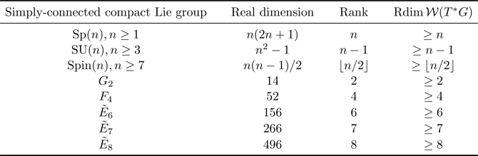
Example 5.25 (Complex projective spaces)
Let us also briefly mention the case of complex projective spaces. The cohomology of  $\Omega \mathbb {CP}^n$ is computed in [Reference SeeligerSee14, Theorem 1.3]. It contains a free subalgebra $\mathbb {Q}[y]$ where $|y|=2n$. On the other hand, as explained in, e.g., [Reference SeeligerSee14, § 3], we have $\Omega \mathbb {CP}^n= S^1 \times \Omega S^{2n+1}$ and, hence, $H_\bullet (\Omega \mathbb {CP}^n) = H_\bullet (S^1) \otimes H_\bullet (\Omega S^{2n+1})$. It is shown in [Reference Briggs and GelinasBG17, Example 5.7] that the characteristic morphism hits the class $1 \otimes v$ of degree $2n$ in $H_\bullet (\Omega \mathbb {CP}^n)$. For degree reasons, the composition of $\mathbb {Q}[y] \to H_{\bullet +2n}(\mathcal {L}\mathbb {CP}^n) \to H_\bullet (\Omega \mathbb {CP}^n)$ must send $y$ to $1 \otimes v$.
By a similar argument to Example 5.22, we find that if  $M=M_1 \times \cdots \times M_k$ where each $M_i$ is a sphere of dimension at least $2$ or a complex projective space of arbitrary dimension, then
 \begin{equation} \operatorname{Rdim} \mathcal{W}(M) \geqslant k. \end{equation}
6. Applications to symplectic geometry
We now describe how the Rouquier dimension of wrapped Fukaya categories is related to certain quantities and operations of geometric interest.
6.1 Embedding monotonicity
An important fact about the Rouquier dimension of Weinstein manifolds is that it is monotonic under Liouville embeddings which are Weinstein up to deformation. To explain this precisely, we begin with the following definition.
Definition 6.1 A Liouville embedding of Liouville domains is a codimension- $0$ smooth embedding
 \begin{equation} i: (X_0^{\operatorname{in}}, \lambda_0^{\operatorname{in}}) \hookrightarrow (X_0, \lambda_0) \end{equation}
where  $i^*\lambda _0= e^{\rho } \lambda _0^{\operatorname {in}} + df$ for some $\rho \in \mathbb {R}$ and $f: X_0^{\operatorname {in}} \to \mathbb {R}$.
We refer to [Reference Ganatra and SiegelGaSi21, § 2.1.3] for a detailed discussion of Liouville embeddings. As explained in [Reference Ganatra and SiegelGaSi21, Lemma 2.2], any Liouville embedding as in Definition 6.1 extends to a family of Liouville embeddings  $i^t: (X_0^{\operatorname {in}}, \lambda _0^{\operatorname {in}}) \hookrightarrow (X_0, \lambda _0^t)$ such that $i=i^0$ and $i^1$ is a strict Liouville embedding, i.e. $(i^1)^* \lambda _0^1 = \lambda _0^{\operatorname {in}}$.
Proposition 6.2 Let  $i: (X_0^{\operatorname {in}}, \lambda ^{\operatorname {in}} ) \subseteq (X_0, \lambda )$ be a Liouville embedding and suppose that $(X_0^{\operatorname {in}}, \lambda ^{\operatorname {in}})$ and $(X_0- i(X_0^{\operatorname {in}}), \lambda )$ are Weinstein up to deformation. Then
 \begin{equation} \operatorname{Rdim} \mathcal{W}(X^{\operatorname{in}}) \leqslant \operatorname{Rdim} \mathcal{W}(X) \end{equation}
where  $X^{\operatorname {in}}, X$ are the completions of $X_0^{\operatorname {in}}, X_0$ respectively.
Proof. As the wrapped Fukaya category is invariant under deformation, we may assume that the embedding is strict, i.e. $i^*\lambda = \lambda ^{\operatorname {in}}$. We may therefore appeal to [Reference Ganatra, Pardon and ShendeGPS22, Proposition 11.2], which constructs a Viterbo restriction functor
 \begin{equation} \operatorname{Tw} \mathcal{W}(X) \to \operatorname{Tw} \mathcal{W}(X^{\operatorname{in}}). \end{equation}
As explained in [Reference Ganatra, Pardon and ShendeGPS22, Proposition 11.2], the hypothesis that the  $X_0^{\operatorname {in}}$ and $X_0- i(X_0^{\operatorname {in}})$ are Weinstein implies that there is, in fact, a quasi-equivalence $\operatorname {Tw} \mathcal {W}(X) /\mathcal {D} \to \operatorname {Tw} \mathcal {W}(X^{\operatorname {in}})$, where $\mathcal {D}$ is a set of objects. The claim now follows from Corollary 2.12 upon passing to $\operatorname {Perf}(-)$.
In the statement of Proposition 6.2, note that the orientation/grading data on  $\mathcal {W}(X^{\operatorname {in}})$ is implicitly induced from the orientation/grading data on $X$.
$X$.
It is natural to ask whether one can drop the hypothesis that  $X_0- i(X_0^{\operatorname {in}})$ is Weinstein Proposition 6.2. We note that Sylvan has proved [Reference SylvanSyl19a] that the Viterbo restriction functor in this setting functor is a homological epimorphism, although it is not clear if this helps.
By combining various upper and lower bounds for  $\operatorname {Rdim}\mathcal {W}(-)$ discussed in the introduction and in the following, it is easy to write down examples of putative embeddings $X_0^{\operatorname {in}} \hookrightarrow X_0$ which are obstructed by $\operatorname {Rdim} \mathcal {W}(-)$. For instance, we have the following.
Example 6.3 Let  $X$ be a Weinstein manifold of real dimension $2(n^2-1)$ admitting a Lefschetz fibration with Weinstein fibers having $< n-2$ critical points. Then $X$ does not contain $T^*SU(n)$ as a Weinstein subdomain.
There is, of course, nothing special about Example 6.3, and there is a plethora of similar examples. It seems unlikely to the authors that examples such as these could be handled using invariants already in the literature. From this perspective,  $\operatorname {Rdim} \mathcal {W}(-)$ is a useful addition to the symplectic topologist's toolkit of embedding obstructions. On the other hand, $\operatorname {Rdim} \mathcal {W}(-)$ has many blind spots. The most obvious defect of $\operatorname {Rdim} \mathcal {W}(-)$ as an embedding obstruction is that it outputs a very limited range of values: indeed, it seems plausible that $\operatorname {Rdim} \mathcal {W}(X^{2n}) \in [0, n]$ (see Corollary 4.17 for a somewhat weaker statement).
6.2 Lefschetz fibrations
We now discuss upper bounds for the Rouquier dimension of wrapped Fukaya categories in terms of the number of critical points of a Lefschetz fibration.
Definition 6.4 [Reference Maydanskiy and SeidelMS10, § 2]
Given a Liouville manifold  $X$, a Lefschetz fibration is a smooth map $f: X\to \mathbb {C}$ having Morse-type critical points and such that $\operatorname {ker} df$ is symplectic away from the critical points. This data is required to satisfy some additional technical conditions at infinity detailed in [Reference Maydanskiy and SeidelMS10, § 2]. A Lefschetz fibration is said to have Weinstein fibers if the general fiber is a Weinstein manifold up to deformation.
There are various essentially equivalent notions of a Lefschetz fibration in the literature. We have adopted the setup of [Reference Maydanskiy and SeidelMS10, § 2] for consistency with [Reference Ganatra, Pardon and ShendeGPS20a, § 1.1].
Definition 6.5 Given a Liouville manifold  $X$ (considered up to Liouville homotopy), we let
 \begin{equation} \operatorname{Lef}_w(X) \in \mathbb{N} \cup \{\infty\} \end{equation}
denote the minimal number of critical points of a Lefschetz fibration on  $X$ with Weinstein fibers. We set $\operatorname {Lef}_w(X)= \infty$ if no such fibration exists.
It was proved by Giroux and Pardon [Reference Giroux and PardonGP17, Theorem 1.10] using quantitative transversality techniques that any Weinstein manifold admits a Lefschetz fibration with Weinstein fibers. Conversely, if a Liouville manifold admits a Lefschetz fibration with Weinstein fibers, then it is Weinstein (this is tautological if one uses [Reference Giroux and PardonGP17, Definition 1.9]). Hence,  $\operatorname {Lef}_w(X) < \infty$ if and only if $X$ admits a Weinstein structure.
Concerning lower bounds, there is a purely topological bound  $\operatorname {rk} H_n(X; \mathbb {Z}) \leqslant \operatorname {Lef}_w(X)$, where $X$ has real dimension $2n$. It is also immediate that $\operatorname {Lef}_w(X)=0$ if and only if $X$ is subcritical, meaning that it splits as a product of Liouville manifolds $(X, \lambda )= (F_0 \times \mathbb {C}, \lambda _0 \times \lambda _{\mathbb {C}})$.
The following proposition, which was explained to us by Y. Barış Kartal, states that the Rouquier dimension gives another lower bound.
Proposition 6.6 Let  $X$ be a Liouville manifold. Then
 \begin{equation} \operatorname{Lef}_w(X) \geqslant \operatorname{Rdim}\mathcal{W}(X) +1. \end{equation}
Proof. We may assume without loss of generality that  $0<\operatorname {Lef}_w(X) = k <\infty$. Fix a Lefschetz fibration $f: X \to \mathbb {C}$ with $k$ critical points and choose a set of thimbles $\{ L_1, \ldots,L_k \}$. These form an exceptional collection for the partially wrapped Fukaya category $\mathcal {W}(X, f^{-1}({\infty }))$ (see [Reference Ganatra, Pardon and ShendeGPS20a, Example 1.4]). According to [Reference Ganatra, Pardon and ShendeGPS22, Corollary 1.17], this exceptional collection is full, meaning that it generates $\mathcal {W}(X, f^{-1}(\{\infty \}))$. It follows by Lemma 2.10 that $\operatorname {Rdim} \mathcal {W}(X, f^{-1}(\{\infty \})) \leqslant k-1$.
It follows from [Reference Ganatra, Pardon and ShendeGPS22, Corollary 3.9] that  $\mathcal {W}(X, f^{-1}(\{\infty \})) = \mathcal {W}(X, {\frak c})$, where ${\frak c}$ is the skeleton of $f^{-1}(\infty )$. The assumption that $f^{-1}(\{\infty \})$ is Weinstein implies that ${\frak c}$ is mostly Legendrian [Reference Ganatra, Pardon and ShendeGPS22, see Definition 1.7]. It then follows from Theorem 3.5, that the natural map $\mathcal {W}(X, f^{-1}(\{\infty \})) \to \mathcal {W}(X)$ is a quotient of $A_\infty$ categories. Corollary 2.12 thus implies that $\operatorname {Rdim} \mathcal {W}(X) \leqslant k-1$.
We do not expect (6.5) to be sharp except in very special cases.
Example 6.7 The affine quadric  $\{z_1^2 + \cdots + z_n^2 +z_{n+1}^2 = 1\}$ with the Liouville structure $\sum y_i\,dx_i$ is isomorphic to $T^*S^n$ as a Liouville manifold. The projection $(z_1, \ldots, z_{n+1}) \mapsto z_{n+1}$ is a Lefschetz fibration with two critical points. Hence $\operatorname {Rdim} \mathcal {W}(T^*S^n) \leqslant 1$. By Example 5.24, this is an equality if $\mathcal {W}(T^*S^n)$ is defined with $\mathbb {Z}/2$-gradings and $\mathbb {Q}$-coefficients.
Although the definition of  $\operatorname {Lef}_w(X)$ only makes sense on Liouville manifolds, it is not a priori clear to what extent this invariant depends on the Liouville structure (recall Lazarev's result ‘ $\operatorname {WMor}(X)=\operatorname {Mor}(X)$’ discussed in the introduction, which implies that $\operatorname {WMor}(X)$ does not depend on the Liouville structure). The following corollary shows that the natural complex analog of ‘ $\operatorname {WMor}(X)=\operatorname {Mor}(X)$’ is false.
Corollary 6.8 There exists a Weinstein manifold  $T^*S^3_{\operatorname {exotic}}$ which is formally isotopic to $T^*S^3$, but such that $\operatorname {Lef}_w(T^* S^3) \neq \operatorname {Lef}_w(T^* S^3_{\operatorname {exotic}})$.
Proof. [Reference Eliashberg, Ganatra and LazarevEGL20, Theorem 4.7] produces a Weinstein manifold  $T^*S^3_{\operatorname {exotic}}$ which contains a flexible Lagrangins $L \simeq \mathbb {T}^3$. This means by definition that L is regular (see [Reference Eliashberg, Ganatra and LazarevEGL20, Definition 3.1]) and, hence, the cobordism $T^*S^3_{\operatorname {exotic}} - T^*_{\leqslant \epsilon }L$ is Weinstein. Now combine Propositions 6.2 and 6.6. It follows that $\operatorname {Lef}_w(T^*S^3_{\operatorname {exotic}}) \geqslant \operatorname {Rdim} \mathcal {W}(T^*S^3_{\operatorname {exotic}}) +1\geqslant \operatorname {Rdim} \mathcal {W}(T^*\mathbb {T}^3)+1 \geqslant 4$ by Example 5.18. On the other hand, we saw in Example 6.7 that $\operatorname {Lef}_w(T^*S^3) \leqslant 2$.
6.3 Rigidity of skeleta
Finally, we prove the quantitative symplectic rigidity result for the skeleton of a Weinstein manifold which was advertised in the introduction.
Proposition 6.9 Let  $(X, \lambda )$ be a Liouville manifold. Suppose that the skeleton ${\frak c}_X$ is mostly Lagrangian and that every component of ${\frak c}_X^{\operatorname {crit}}$ admits a generalized cocore.
Let  $\phi : X \to X$ be a Hamiltonian symplectomorphism. If ${\frak c}_X \cap \phi ({\frak c}_X)= {\frak c}_X^{\operatorname {crit}} \cap \phi ({\frak c}_X^{\operatorname {crit}})$ and these intersection points are transverse (a generic condition on $\phi$), then
 \begin{equation} |{\frak c}_X \cap \phi({\frak c}_X)| \geqslant \operatorname{Rdim}\mathcal{W}(X) +1. \end{equation}
Proof. We consider the Liouville manifold  $(\overline {X} \times X, -\lambda \oplus \phi _* \lambda )$ which has skeleton ${\frak c}_X \times \phi ({\frak c}_X)$. Let $\Delta \subseteq \overline {X} \times X$ be the diagonal. By assumption, $\Delta$ intersects ${\frak c}_X \times \phi ({\frak c}_X)$ at finitely many points. Suppose there are $r \geqslant 0$ such points.
Consider the diffeomorphism
 \begin{align} (\overline{X} \times X, -\lambda \oplus \phi_* \lambda) &\to (\overline{X} \times X, -\lambda \oplus \lambda) \end{align}
 \begin{align} (x_1, x_2) &\mapsto (x_1, \phi^{-1}(x_2)), \end{align}
which sends  $\Delta$ to the Lagrangian $L= \{(x, \phi ^{-1}(x)\}$.
We now apply Theorem 3.6. This produces a resolution of  $L$ of length $r \geqslant 0$ by generalized cocores of ${\frak c}_{\overline {X} \times X}= {\frak c}_X \times {\frak c}_X$. Observe that one can choose these generalized cocores to be products of generalized cocores of ${\frak c}_X$. As $L$ is isotopic to $\Delta$ through a compactly supported Lagrangian isotopy, they define isomorphic objects in $\mathcal {W}(\overline {X} \times X)$. Applying Theorem A.2, we obtain a resolution of the diagonal bimodule of length $r$ by Yoneda bimodules. The conclusion now follows from Lemma 2.13.
Remark 6.10 The assumption that  ${\frak c}_X^{\operatorname {crit}}$ and $\phi ({\frak c}_X^{\operatorname {crit}})$ intersect transversally is used in the proof of Proposition 6.9 when appealing to Theorem 3.6. However, we do not know whether this assumption is necessary for the conclusion of the theorem to hold.
The proof of Proposition 6.9 can actually be adapted to derive lower bounds for  $|{\frak c}_X \cap \phi ({\frak c}_X)|$ which do not involve the Rouquier dimension of $\mathcal {W}(X)$.
For example, suppose that  $\mathcal {W}(X)$ admits a non-zero proper module. Then we claim $|{\frak c}_X \cap \phi ({\frak c}_X)|>1$. Indeed, if $r=0$, then $\mathcal {W}(X)=0$. If $r=1$, then the proof of Proposition 6.9 implies that the diagonal bimodule is isomorphic to $\mathcal {Y}^l_K \otimes _k \mathcal {Y}^r_L$ for some objects $K, L$ of $\mathcal {W}(X)$. Convolving with $\mathcal {P}$, we find that $H^\bullet (P, P)= H^\bullet (K, K) \otimes H^\bullet (\mathcal {Y}^r_L, P)$. Hence, $H^\bullet (K, K)$ is finite-dimensional. On the other hand, the convolution argument of Lemma 2.13 proves that $K$ split-generates $\mathcal {W}(X)$. Thus, $\mathcal {W}(X)$ is proper, which contradicts the main result of [Reference GanatraGan1221].
Similarly, one can show that  $|{\frak c}_X \cap \phi ({\frak c}_X)|$ is strictly greater than the dimension of the image of $K_0(\operatorname {Prop} \mathcal {C})$ in $K_0(\operatorname {Perf} \mathcal {C})$.
Example 6.11 If  $X$ contains an orientable closed exact Lagrangian, then this defines a proper module over $\mathcal {W}(X)$ (where we work with $\mathbb {Z}/2$ gradings and $\mathbb {Z}/2$ coefficients). Hence, $|{\frak c}_X \cap \phi ({\frak c}_X)| \geqslant 2$.
Acknowledgements
We are indebted to Daniel Álvarez-Gavela for answering countless questions about arborealization, Vivek Shende for help with microlocal sheaves and homological mirror symmetry of toric varieties, Srikanth Iyengar for discussions and comments related to § 5.2, Y. Barış Kartal for showing us the proof of Proposition 6.6 and for useful discussions related to § 4.5, and John Pardon for many helpful conversations about various aspects of the paper. In addition, we would like to thank Denis Auroux, Petter Bergh, Georgios Dimitroglou Rizell, Sheel Ganatra, Wahei Hara, Oleg Lazarev, David Nadler, Amnon Neeman, and Dmitri Orlov for answering our questions at various points in this project. SB would like to express deep gratitude to his advisor John Pardon for constant encouragement and support. LC learned about Question 1.4 from Zhengyi Zhou and would like to thank him for many enjoyable and informative discussions. LC would also like to thank Y. Barış Kartal for teaching him much of what he knows about  $A_\infty$ categories. Finally, we would like to thank the anonymous referee for many useful comments which have significantly improved this paper.
Appendix A
The purpose of this Appendix is to prove Theorem A.2. Our proof is essentially a modification of [Reference Ganatra, Pardon and ShendeGPS22] and [Reference GanatraGan12, § 9], but we include it for completeness.
Remark A.1 After the original version of this paper first appeared, Ganatra, Pardon, and Shende posted a substantially revised version of [Reference Ganatra, Pardon and ShendeGPS22] from which a proof of Theorem A.2 can straightforwardly be extracted.
Let  $(X, \lambda )$ be a Liouville manifold and let $\mathcal {W}(X)$ be its wrapped Fukaya category. Let ${\mathcal {W}(\overline {X} \times X)}$ denote the wrapped Fukaya category of the product $(\overline {X} \times X, -\lambda \oplus \lambda )$.
If  $K$ and $L$ are cylindrical Lagrangians in $X$, their product $K \times L$ is not a cylindrical Lagrangian in $\overline {X} \times X$ in general. However, following [Reference Ganatra, Pardon and ShendeGPS22, § 7.2], the product can be ‘cylindrized’. This results in a cylindrical Lagrangian $K \tilde {\times } L$ which behaves like $K \times L$ in the Floer-theoretic sense; see Lemma A.8. If $K, L$ are invariant under the Liouville flow (e.g. they could be cocores), then $K \times L = K \tilde {\times } L$.
Let  $\mathcal {W}_{\operatorname {cyl}}(\overline {X} \times X) \subset \mathcal {W}(\overline {X} \times X)$ denote the smallest full, replete subcategory of $\mathcal {W}(\overline {X} \times X)$ containing the diagonal $\Delta \subset \overline {X} \times X$ and all cylindrized products (i.e. all objects of the form $K \tilde {\times } L$).
Theorem A.2 There exists a fully faithful  $A_\infty$ functor
 \begin{equation} \mathcal{F}: \mathcal{W}_{\operatorname{cyl}}(\overline{X} \times X) \to (\mathcal{W}(X), \mathcal{W}(X))-\operatorname{mod} \end{equation}
which satisfies the following properties:
(i) the image of the diagonal
$\Delta \subseteq \overline {X} \times X$ is the diagonal bimodule;(ii) the image of any product Lagrangian
$K \times L$ is the Yoneda bimodule $\mathcal {Y}^l_K \otimes _k \mathcal {Y}^r_L$.


Corollary A.3 If  $X$ is Weinstein, then $\mathcal {F}$ extends to a fully faithful functor $\operatorname {Tw}\mathcal {W}(\overline {X} \times X) \to (\mathcal {W}(X), \mathcal {W}(X))-\operatorname {mod}.$
The proof of Theorem A.2 occupies the remainder of this Appendix.
Definition A.4 (Wrapping category of $(X, \lambda )$)

Define the wrapping category  $((X, \lambda ) \leadsto -)^+$ of $(X, \lambda )$ as follows. The objects of $((X, \lambda ) \leadsto -)^+$ are Hamiltonian isotopies of $X$ generated by Hamiltonians $\{ H_t \}_{0 \leqslant t \leqslant 1}$ such that $H_t$ is linear at infinity. Given two objects $\{ H_t \}_{0 \leqslant t \leqslant 1}$ and $\{ H^{\prime }_t \}_{0 \leqslant t \leqslant 1}$ in $((X, \lambda ) \leadsto -)^+$, denote by $\phi _{H_t}$ and $\phi _{H^{\prime }_t}$, respectively, the Hamiltonian diffeomorphisms generated by them. Morphisms from $\{ H_t \}_{0 \leqslant t \leqslant 1}$ to $\{ H^{\prime }_t \}_{0 \leqslant t \leqslant 1}$ are given by Hamiltonian diffeomorphisms satisfying $\phi _{H^{\prime }_t} = \phi _{H_t} \sharp \phi _{\tilde {H}_t}$ and the generating Hamiltonians $\{ \tilde {H}_t \}_{0 \leqslant t \leqslant 1}$ are positive and linear at infinity. Here $\phi _{H_t} \sharp \phi _{\tilde {H}_t}$ means the Hamiltonian diffeomorphism generated by $H_t \sharp \tilde {H}_t (x) = H_t(x) + \tilde {H}_t((\Phi ^t_{H_t})^{-1}(x))$ and $\Phi ^t_{H_t}$ is the time- $t$ flow of the Hamiltonian vector field of $H_t$.
Recall that a category  $\mathcal {C}$ is filtered if
(i)
$\mathcal {C}$ is non-empty;(ii) for every pair of objects
$x, y \in \mathcal {C}$, there exists an object $z \in \mathcal {C}$ and morphisms $x \rightarrow z, y \rightarrow z$;(iii) for every pair of morphisms
$f,g: x \rightarrow y$, there exists an object $z \in \mathcal {C}$ and a morphism $h: y \rightarrow z$ such that $h \circ f = h \circ g$.


A filtered category  $\mathcal {C}$ is has countable cofinality if there exists a cofinal functor $\mathbb {Z}_{\geqslant 0} \rightarrow \mathcal {C}$.
Lemma A.5 The category  $((X, \lambda ) \leadsto -)^+$ is filtered and has countable cofinality.
Proof. The proof that the category is filtered proceeds exactly as [Reference Ganatra, Pardon and ShendeGPS20a, Lemma 3.27], except replacing the Lagrangian isotopies by Hamiltonian isotopies. That  $((X, \lambda ) \leadsto -)^+$ has countable cofinality can be proved by choosing a countable family of linear Hamiltonians with slope going to infinity.
Lemma A.6 Consider the diagonal  $\Delta \subset \overline {X} \times X$ as a cylindrical Lagrangian. Let $(\Delta \leadsto -)^+$ be the positive wrapping category of $\Delta$ in the sense of [Reference Ganatra, Pardon and ShendeGPS20a, § 3.4]. Denote by $\pi _1$ and $\pi _2$ the projection from $\overline {X} \times X$ to the first and second factors, respectively. Then the functor from $((X, \lambda ) \leadsto -)^+$ to $(\Delta \leadsto -)^+$ by taking a generating Hamiltonian $H_{t}$ to the Lagrangian isotopy of $\Delta$ which is generated by $\pi _1^{*}H_{1-t/2} + \pi _2^{*}H_{t/2}$ is cofinal.
Proof. This holds by inspecting the definitions.
We introduce a category  $\widetilde {\mathcal {O}}^{\operatorname {prod}}_{\overline {X} \times X}$ following [Reference Ganatra, Pardon and ShendeGPS22, § 8.2]. Fix a countable collection of Lagrangians $\tilde {I}^{\operatorname {prod}}_{\overline {X} \times X}$ in $\overline {X} \times X$ consisting of $\Delta$ and product Lagrangians $K \times L \subset \overline {X} \times X$ which represent every pair of isotopy classes. For the diagonal $\Delta$, choose a countable cofinal family $\Delta = \Delta ^{(0)} \leadsto \Delta ^{(1)} \leadsto \cdots$ in $(\Delta \leadsto -)^+$ induced from $((X, \lambda ) \leadsto -)^+$ as in Lemma A.6. In addition, choose cofinal wrappings $K = K^{(0)} \leadsto K^{(1)} \leadsto \cdots$ and $L = L^{(0)} \leadsto L^{(1)} \leadsto \cdots$. Then the category $\widetilde {\mathcal {O}}^{\operatorname {prod}}_{\overline {X} \times X}$ has objects given by $\mathbb {Z}_{\geqslant 0} \times \tilde {I}^{\operatorname {prod}}_{\overline {X} \times X}$, which are either of the form $\Delta ^{(i)}$ or $K^{(i)} \times L^{(i)}$. The objects of $\widetilde {\mathcal {O}}^{\operatorname {prod}}_{\overline {X} \times X}$ admits a total order induced from $\mathbb {Z}_{\geqslant 0}$.
Note that by choosing the wrappings generically, we can assume that for any pair of Lagrangians in  $\widetilde {\mathcal {O}}^{\operatorname {prod}}_{\overline {X} \times X}$, they intersect transversally and are disjoint at infinity with distance uniformly bounded from below. Using generic product almost complex structures, as they induce uniformly bounded geometry, one can define $A_{\infty }$ operations on $\widetilde {\mathcal {O}}^{\operatorname {prod}}_{\overline {X} \times X}$ by counting suitable holomorphic discs based on the compactness arguments in [Reference Ganatra, Pardon and ShendeGPS20a, Proposition 3.19]. Of course, the morphism spaces are given by the Floer cochain complexes. The wrappings define a collection of continuation elements (see [Reference Ganatra, Pardon and ShendeGPS20a, Definition 3.25]) $C_{\operatorname {prod}}$ inside the Floer cohomology groups $HF^{0}(K^{(i+1)} \times L^{(i+1)}, K^{(i)} \times L^{(i)})$ and $HF^{0}(\Delta ^{(i+1)}, \Delta ^{(i)})$. Then we define an $A_{\infty }$ category by localizing $\widetilde {\mathcal {O}}^{\operatorname {prod}}_{\overline {X} \times X}$ along $C_{\operatorname {prod}}$:
 \begin{equation} \widetilde{\mathcal{W}}^{\operatorname{prod}}(\overline{X} \times X) := \widetilde{\mathcal{O}}^{\operatorname{prod}}_{\overline{X} \times X}[C^{-1}_{\operatorname{prod}}]. \end{equation}
 By construction and [Reference Ganatra, Pardon and ShendeGPS20a, Lemma 3.37], the following isomorphisms hold in  $\widetilde {\mathcal {W}}^{\operatorname {prod}}(\overline {X} \times X)$ (this is parallel to the computations in [Reference GanatraGan12, § 8.1] under the ‘quadratic’ setup):
 \begin{gather} \operatorname{hom}^{\bullet}(\Delta, \Delta) \cong SH^{\bullet}(X), \end{gather}
 \begin{gather} \operatorname{hom}^{\bullet}(K \times L, \Delta) \cong HW^{\bullet}(L, K), \operatorname{hom}^{\bullet}(\Delta, K \times L) \cong HW^{\bullet}(K, L), \end{gather}
 \begin{gather} \operatorname{hom}^{\bullet}(K \times L, K' \times L') \cong HW^{\bullet}(K, K') \otimes HW^{\bullet}(L, L'). \end{gather}
Proposition A.7 There exists a fully faithful  $A_{\infty }$ functor $\mathcal {F}^{\operatorname {prod}}: \widetilde {\mathcal {W}}^{\operatorname {prod}}(\overline {X} \times X) \to (\mathcal {W}(X), \mathcal {W}(X))-\operatorname {mod}$ which satisfies the following properties:
(i) the image of the diagonal
$\Delta \subseteq \overline {X} \times X$ is the diagonal bimodule;(ii) the image of any product Lagrangian
$K \times L$ is the Yoneda bimodule $\mathcal {Y}^l_K \otimes _k \mathcal {Y}^r_L$.


Proof. Recall that the wrapped Fukaya category  $\mathcal {W}(X)$ is defined as a localization $\mathcal {O}_X [C^{-1}]$. Here $\mathcal {O}_{X}$ is an $A_{\infty }$ category whose objects are given by $\mathbb {Z}_{\geqslant 0} \times I_{X}$, where $I_X$ is a countable collection of cylindrical Lagrangians in $X$ representing all isotopy classes and for each Lagrangian $L \in I_X$ we have a cofinal wrapping sequence $L = L^{(0)} \leadsto L^{(1)} \leadsto \cdots$. The set of morphisms $C$ consists of continuation elements in $HF^{0}(L^{(i+1)}, L^{(i)})$. For details, see [Reference Ganatra, Pardon and ShendeGPS22, § 5.5].
Without loss of generality, we can assume that the product Lagrangians in the set  $\tilde {I}^{\operatorname {prod}}_{\overline {X} \times X}$ in $\overline {X} \times X$ are all given by product of Lagrangians from $I_X$. Then we can define an $A_{\infty }$ functor
 \begin{equation} \widetilde{\mathcal{O}}^{\operatorname{prod}}_{\overline{X} \times X} \rightarrow (\mathcal{O}_X, \mathcal{O}_X)-\operatorname{mod} \end{equation}
by considering quilted holomorphic maps as in [Reference GanatraGan12, § 9]. More precisely, for any Lagrangian  $\mathcal {L} \in \widetilde {\mathcal {O}}^{\operatorname {prod}}_{\overline {X} \times X}$, it defines an $A_{\infty }$ bimodule $\mathcal {M}_{\mathcal {L}}$ over $\mathcal {O}_X$ whose morphism space associates to a pair of Lagrangians $K, L \in \mathcal {O}_X$ the Floer cochain complex
 \begin{equation} \operatorname{hom}_{\widetilde{\mathcal{O}}^{\operatorname{prod}}_{\overline{X} \times X}}^{\bullet}(K \times L, \mathcal{L}). \end{equation}
The  $A_{\infty }$ operations are defined by counting quilted holomorphic maps into $\overline {X} \times X$ with seam along the Lagrangian $\mathcal {L}$; see [Reference Ganatra, Pardon and ShendeGPS22, Figure 19] without inserting marked points along the seam on the left picture and replacing both $X^{-}\ {\rm and}\ Y$ by $X$. The almost complex structures are of product type and are chosen generically. Once again, the compactness arguments from [Reference Ganatra, Pardon and ShendeGPS20a, Proposition 3.19] and [Reference Ganatra, Pardon and ShendeGPS22, § 8.2] guarantee that the relevant moduli spaces which define $\mathcal {M}_{\mathcal {L}}$ and verify the $A_{\infty }$ relations are compact. To complete the definition of the $A_{\infty }$ functor $\widetilde {\mathcal {O}}^{\operatorname {prod}}_{\overline {X} \times X} \rightarrow (\mathcal {O}_X, \mathcal {O}_X)-\operatorname {mod}$, it suffices to consider quilted holomorphic maps with marked points inserted along the seam, which are exactly the left picture of [Reference Ganatra, Pardon and ShendeGPS22, Figure 19] after replacing both $X^{-}$ and $Y$ by $X$. Note that we allow Lagrangians $\Delta ^{(i)}$ as markings on the seam, but they do not impose further difficulties in the construction. By definition, this functor takes the (strict) diagonal Lagrangian $\Delta$ to the diagonal bimodule $\Delta _{\mathcal {O}_X}$ and takes the product Lagrangian $K \times L$ to the Yoneda bimodule $\mathcal {Y}^l_K \otimes _k \mathcal {Y}^r_L$ over the category $\mathcal {O}_X$.
The localization functor  $\mathcal {O}_X \rightarrow \mathcal {W}(X)$ induces an $A_{\infty }$ functor
 \begin{equation} (\mathcal{O}_X, \mathcal{O}_X)-\operatorname{mod} \to (\mathcal{W}(X), \mathcal{W}(X))-\operatorname{mod} \end{equation}
and its composition with the functor defined in the previous paragraph defines an  $A_{\infty }$ functor
 \begin{equation} \widetilde{\mathcal{O}}^{\operatorname{prod}}_{\overline{X} \times X} \rightarrow (\mathcal{W}(X), \mathcal{W}(X))-\operatorname{mod}. \end{equation}
Using the definition of continuation elements in  $C_{\operatorname {prod}}$, we see that the functor descends to an $A_{\infty }$ functor
 \begin{equation} \mathcal{F}^{\operatorname{prod}}: \widetilde{\mathcal{W}}^{\operatorname{prod}}(\overline{X} \times X) \to (\mathcal{W}(X), \mathcal{W}(X))-\operatorname{mod} \end{equation}
by the universal property of localization. The statements are proved because of (A.4) and (A.5).
Lemma A.8 There exists a fully faithful ‘cylindrization’  $A_{\infty }$ functor $\widetilde {\mathcal {W}}^{\operatorname {prod}}(\overline {X} \times X) \to \mathcal {W} (\overline {X} \times X)$ which takes the diagonal to the diagonal and takes products $K \times L$ to their cylindrization $K \tilde {\times } L$. In particular, this functor is a quasi-equivalence onto $\mathcal {W}_{\operatorname {cyl}}(\overline {X} \times X)$.
Proof. Let  $\mathcal {O}_{\overline {X} \times X}$ be the pre-localized category whose quotient defines $\mathcal {W}(\overline {X} \times X)$. The $A_{\infty }$ functor
 \begin{equation} \widetilde{\mathcal{O}}^{\operatorname{prod}}_{\overline{X} \times X} \to \mathcal{O}_{\overline{X} \times X} \end{equation}
is defined using the extension of the  $(\mathcal {O}^{\operatorname {prod}}_{\overline {X} \times X}, \mathcal {O}_{\overline {X} \times X})$-bimodule $\mathcal {B}$ from [Reference Ganatra, Pardon and ShendeGPS22, § 8.2] by adding the diagonal Lagrangian. Note that by our choice of wrappings of the diagonal, all $\Delta ^{(i)}$ for $i \geqslant 0$ are cylindrical and obviously the diagonal is taken to the diagonal. The comparisons between Floer cochain complexes as in [Reference Ganatra, Pardon and ShendeGPS22, § 8.2] carry over without change so the induced functor from $\mathcal {B}$ is an equivalence onto its image. The desired functor is constructed by localization and it is a quasi-equivalence onto $\mathcal {W}_{\operatorname {cyl}}(\overline {X} \times X)$ by definition.


 Open access