


Impact Statement
Structural health monitoring (SHM) utilizes sensor technology to identify and detect potential damage to critical infrastructure like bridges. However, the available measurements can be affected by external factors such as temperature, requiring data-driven methods to account for these influences. This study presents an interpretable framework based on functional data analysis to effectively utilize the data’s structure and characteristics, including daily and seasonal patterns, when adjusting for confounding effects. Many existing methods for removing environmental effects are encompassed as special cases. Additionally, damage-sensitive features are readily accessible and can be monitored using state-of-the-art control charts.
1. Introduction
Structural health monitoring (SHM) employs sensor technologies to collect data from structures such as bridges to detect, localize, or quantify damage (Deraemaeker et al., Reference Deraemaeker, Reynders, De Roeck and Kullaa2008; Kullaa, Reference Kullaa2011; Hu et al., Reference Hu, Moutinho, Caetano, Magalhães and Cunha2012; Magalhães et al., Reference Magalhães, Cunha and Caetano2012). These field measurements often exhibit missing data and are influenced by environmental and operational factors such as temperature, wind, humidity, or traffic load (Wang et al., Reference Wang, Yang, Yi, Zhang and Han2022). Multiple studies, including Wang et al. (Reference Wang, Yang, Yi, Zhang and Han2022), Han et al. (Reference Han, Ma, Xu and Liu2021) and the references therein, identify temperature as a predominant factor affecting structural stiffness and material properties due to thermal expansion and contraction (Han et al., Reference Han, Ma, Xu and Liu2021). Consequently, data-driven methods are essential to take these confounding effects in SHM data analysis into account.
With respect to separating temperature-induced responses from structural responses, it can be distinguished between so-called “input–output” methods and “output-only” approaches (Wang et al., Reference Wang, Yang, Yi, Zhang and Han2022). In the first case, both the sensor measurements and observations of the confounding variables, such as temperature, are considered, while in the latter case, as the name suggests, only the responses of the structures are used, often using projection methods such as principal component analysis (PCA). Among input–output methods, a prevalent approach is regressing sensor measurements on environmental or operational variables, also known under the name response surface modeling. Then, following the so-called “subtraction method,” the predicted sensor data is subtracted from the actually observed data, and the residuals are used for further analysis. For fitting regression function(s) to the data, various methods have been used in the SHM literature, ranging from simple linear or polynomial regression to advanced machine learning approaches such as artificial neural networks, see Avci et al. (Reference Avci, Abdeljaber, Kiranyaz, Hussein, Gabbouj and Inman2021). However, often, these methods ignore that output data may exhibit daily or yearly patterns or that error terms are correlated over time, e.g., if estimating unknown parameters through least-squares (Cross et al., Reference Cross, Koo, Brownjohn and Worden2013; Maes et al., Reference Maes, Van Meerbeeck, Reynders and Lombaert2022). In other cases, rather restrictive parametric assumptions known from time series analysis are made (Hou and Xia, Reference Hou and Xia2021). Furthermore, input–output and output-only methods are typically considered to be completely different approaches. An overarching framework is still missing where, for instance, it is possible to switch from one approach to the other without changing the downstream monitoring procedure, or the common situation can be handled where measurements are available only for a few confounding variables while others are unobserved or unknown.
In light of this, we will present a novel functional data analysis (FDA) perspective to address these challenges in SHM. FDA has been an area of intensive methodological research over the last two or three decades. For an introduction to FDA in general and an overview of recent developments, the works by Ramsay and Silverman (Reference Ramsay and Silverman2005), Wang et al. (Reference Wang, Chiou and Müller2016), and Gertheiss et al. (Reference Gertheiss, Rügamer, Liew and Greven2024) are recommended. Existing applications of FDA within SHM are reviewed by Momeni and Ebrahimkhanlou (Reference Momeni and Ebrahimkhanlou2022). In SHM, so far, FDA has primarily been used for distributional regression and change point detection. For instance, Chen et al. (Reference Chen, Bao, Tang, Chen and Li2020) used FDA to segment data by time and analyze corresponding probability density functions through warping functions and functional principal component analysis (FPCA). Other notable contributions include the works by Chen et al. (Reference Chen, Bao, Li and Spencer2018), Chen et al. (Reference Chen, Bao, Li and Spencer2019), and Chen et al. (Reference Chen, Lei, Bao, Deng, Zhang and Li2021), who developed methods for imputing missing data using distribution-to-distribution and distribution-to-warping functional regression, and Lei et al. (Reference Lei, Chen and Li2023a), Lei et al. (Reference Lei, Chen, Li and Wei2023c), and Lei et al. (Reference Lei, Chen, Li and Wei2023b) focused on outlier detection and change-point detection in FDA. Jiang et al. (Reference Jiang, Wan, Yang, Ding and Xue2021) modeled temperature-induced strain relationships using warping functions and FPCA.
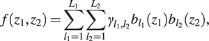
To elucidate our functional perspective, consider Figure 1. Similar plots in SHM studies, such as Xia et al. (Reference Xia, Chen, Weng, Ni and Xu2012), Xia et al. (Reference Xia, Zhang, Tian and Zhang2017), and Zhou et al. (Reference Zhou, Serban and Gebraeel2011), have been used to illustrate the relationship between natural frequencies, strain or displacement, and temperature. However, to the best of our knowledge, this functional nature of the data has never been exploited in SHM when correcting for confounding effects. The data in Figure 1 are from the KW51 railway bridge (Maes and Lombaert, Reference Maes and Lombaert2020), near Leuven, Belgium, monitored from October 2, 2018 to January 15, 2020, including a retrofitting period from May 15 to September 27, 2019. This dataset contains hourly natural frequencies and steel surface temperature (more details on the bridge will be given in Section 4). The top-right panel of Figure 1 shows the bridge’s natural frequency (mode 6) for selected days before retrofitting. It appears plausible to assume that there is some underlying daily pattern common to all profiles, which might be caused by environmental influences that may follow some recurring pattern as well. Those patterns and relationships can be further analyzed through FDA, among other things, by regressing the natural frequency profiles on the temperature curves shown in the bottom-left panel of Figure 1. From the colors, it is already visible that there is a negative association between temperature and the natural frequency, meaning that lower temperatures lead to a higher frequency; compare, e.g., Xia et al. (Reference Xia, Hao, Zanardo and Deeks2006), Xia et al. (Reference Xia, Chen, Weng, Ni and Xu2012). The bottom-right panel shows the resulting error profiles when using a conventional, non-functional piecewise linear model to account for this effect, as done by Maes et al. (Reference Maes, Van Meerbeeck, Reynders and Lombaert2022).
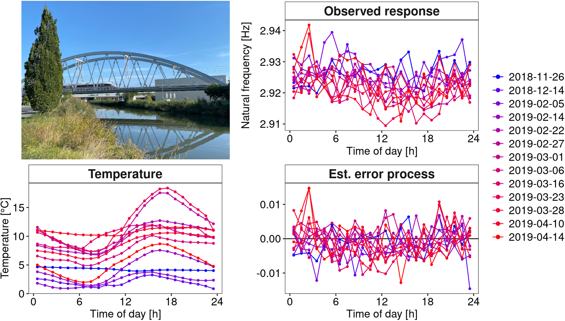
Figure 1. KW51 Bridge from the south side in September 2024 (top-left). The natural frequency of mode 6 for some selected days before the retrofitting started (top-right) and the corresponding steel temperature curves (bottom-left). If a simple piecewise linear model is used for temperature adjustment, the error profiles (bottom-right) are obtained.
If considering entire daily profiles rather than individual measurements as the sampling instances, this regression task is called “function-on-function” regression. In the statistical process monitoring (SPM) literature, it is part of so-called profile monitoring, see Woodall et al. (Reference Woodall, Spitzner, Montgomery and Gupta2004), Woodall (Reference Woodall2007), Maleki et al. (Reference Maleki, Amiri and Castagliola2018) for detailed reviews on that topic. Current state-of-the-art methodologies, such as the (linear) functional regression control chart (FRCC) by Centofanti et al. (Reference Centofanti, Lepore, Menafoglio, Palumbo and Vantini2021), have limitations in SHM applications, where the relationship between temperature and natural frequencies is often nonlinear (Han et al., Reference Han, Ma, Xu and Liu2021). Additionally, by integrating over the entire domain (i.e., the entire day in Figure 1), the employed functional linear model allows “future observations” to influence the current value of the response (Wittenberg et al., Reference Wittenberg, Knoth and Gertheiss2024). Specifically, if (material) temperature data is available directly from the structure itself instead of ambient temperature, it appears more plausible to use a so-called concurrent model, where the response data at time point $ t $
depends only on the steel temperature at time
$ t $
depends only on the steel temperature at time $ t $
, not the temperature over the entire day. Finally, the assumption of complete datasets, e.g., made in Capezza et al. (Reference Capezza, Centofanti, Lepore, Menafoglio, Palumbo and Vantini2023), is impractical because SHM sensor data often exhibit dropouts due to power or sensor failure. To address these challenges often found in SHM, this paper will consider the very general framework of functional additive mixed models (Scheipl et al., Reference Scheipl, Staicu and Greven2015; Greven and Scheipl, Reference Greven and Scheipl2017) instead of the common functional linear models used by Centofanti et al. (Reference Centofanti, Lepore, Menafoglio, Palumbo and Vantini2021) and Capezza et al. (Reference Capezza, Centofanti, Lepore, Menafoglio, Palumbo and Vantini2023). By doing so, this paper also provides methodological novelty concerning profile monitoring in a more general sense. Besides the regression task, the functional perspective on SHM data offers an elegant way of “de-noising” the data and extracting features through functional principal component scores that can be used as inputs to advanced multivariate control charts. The methods presented in this article can be applied directly to sensor measurements (e.g., strains, inclinations, accelerations) or extracted damage-sensitive features (e.g., eigenfrequencies). That is why this paper will use the more general term “system outputs.” In summary, using the methods discussed, we can model (i) recurring daily and yearly patterns as well as (ii) confounding effects flexibly and interpretably. Furthermore, the presented functional approach also accounts for (iii) correlations and (iv) heteroscedasticity within error profiles. Finally, it will (v) extract covariate-adjusted features from the system outputs and (vi) unify all these aspects within a coherent statistical framework called Covariate-Adjusted Functional Data Analysis for SHM (CAFDA-SHM). This combined approach includes subtraction methods, PCA-based projections (both often used in SHM), and the FRCC in one universal framework, encompassing multiple aspects that have only been considered partially in previous approaches.
$ t $
, not the temperature over the entire day. Finally, the assumption of complete datasets, e.g., made in Capezza et al. (Reference Capezza, Centofanti, Lepore, Menafoglio, Palumbo and Vantini2023), is impractical because SHM sensor data often exhibit dropouts due to power or sensor failure. To address these challenges often found in SHM, this paper will consider the very general framework of functional additive mixed models (Scheipl et al., Reference Scheipl, Staicu and Greven2015; Greven and Scheipl, Reference Greven and Scheipl2017) instead of the common functional linear models used by Centofanti et al. (Reference Centofanti, Lepore, Menafoglio, Palumbo and Vantini2021) and Capezza et al. (Reference Capezza, Centofanti, Lepore, Menafoglio, Palumbo and Vantini2023). By doing so, this paper also provides methodological novelty concerning profile monitoring in a more general sense. Besides the regression task, the functional perspective on SHM data offers an elegant way of “de-noising” the data and extracting features through functional principal component scores that can be used as inputs to advanced multivariate control charts. The methods presented in this article can be applied directly to sensor measurements (e.g., strains, inclinations, accelerations) or extracted damage-sensitive features (e.g., eigenfrequencies). That is why this paper will use the more general term “system outputs.” In summary, using the methods discussed, we can model (i) recurring daily and yearly patterns as well as (ii) confounding effects flexibly and interpretably. Furthermore, the presented functional approach also accounts for (iii) correlations and (iv) heteroscedasticity within error profiles. Finally, it will (v) extract covariate-adjusted features from the system outputs and (vi) unify all these aspects within a coherent statistical framework called Covariate-Adjusted Functional Data Analysis for SHM (CAFDA-SHM). This combined approach includes subtraction methods, PCA-based projections (both often used in SHM), and the FRCC in one universal framework, encompassing multiple aspects that have only been considered partially in previous approaches.
The remainder of the article is structured as follows. In Section 2, our functional data approach is introduced, and our model training and monitoring workflow is presented. The results of a Monte Carlo simulation study validating the developed methods are presented in Section 3. A structural health monitoring application for dynamic response data of the KW51 railway bridge and a second case study for a quasi-static response of a reinforced concrete bridge can be found in Section 4, respectively. Section 5 offers some concluding remarks. Appendix A provides some further modeling options beyond Section 2. For researchers and practitioners who want to apply the newly proposed methods, the code is open source and publicly available at https://github.com/wittenberg/CAFDA-SHM_code.
2. A functional data approach for modeling and monitoring system outputs
2.1. Basic model structure
The model we assume for “in-control” (IC) data has the following basic form. To keep things simple, we first restrict ourselves to a single, functional covariate $ {z}_j(t) $
, e.g., denoting the temperature at time
$ {z}_j(t) $
, e.g., denoting the temperature at time $ t\in \mathcal{T},\mathcal{T}=\left(0\mathrm{h},24\mathrm{h}\right] $
, and day
$ t\in \mathcal{T},\mathcal{T}=\left(0\mathrm{h},24\mathrm{h}\right] $
, and day $ j $
, and a single system output
$ j $
, and a single system output $ {u}_j(t) $
. The latter could be a rather raw sensor measurement (yet preprocessed in some sense), such as strain or inclination data, or extracted features, such as natural frequencies. Then, we assume the basic model
$ {u}_j(t) $
. The latter could be a rather raw sensor measurement (yet preprocessed in some sense), such as strain or inclination data, or extracted features, such as natural frequencies. Then, we assume the basic model
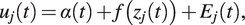 $$ {u}_j(t)=\alpha (t)+f\left({z}_j(t)\right)+{E}_j(t), $$
where $ \alpha (t) $
is a fixed functional intercept,
$ \alpha (t) $
is a fixed functional intercept, $ f\left({z}_j(t)\right) $
is a fixed, potentially nonlinear effect of temperature, and
$ f\left({z}_j(t)\right) $
is a fixed, potentially nonlinear effect of temperature, and $ {E}_j(t) $
is a day-specific, functional error term with zero mean and a common covariance, i.e.,
$ {E}_j(t) $
is a day-specific, functional error term with zero mean and a common covariance, i.e., $ \unicode{x1D53C}\left({E}_j(t)\right)=0 $
,
$ \unicode{x1D53C}\left({E}_j(t)\right)=0 $
, $ \mathrm{Cov}\left({E}_j(s),{E}_j(t)\right)=\Sigma \left(s,t\right) $
,
$ \mathrm{Cov}\left({E}_j(s),{E}_j(t)\right)=\Sigma \left(s,t\right) $
, $ s,t\in \mathcal{T} $
. In the FDA framework used here, sampling instances are days instead of single measurement points, and the daily profiles are considered the quantities of interest. This model has two advantages over scalar-on-scalar(s) regression as typically used for response surface modeling in SHM:
$ s,t\in \mathcal{T} $
. In the FDA framework used here, sampling instances are days instead of single measurement points, and the daily profiles are considered the quantities of interest. This model has two advantages over scalar-on-scalar(s) regression as typically used for response surface modeling in SHM:
-
• The functional intercept $ \alpha (t) $
captures recurring daily patterns that cannot be explained through the available environmental or operational variables, e.g., because the factors causing them are not recorded/available. In the case of long-term monitoring, we may extend the one-dimensional
$ \alpha (t) $
to a two-dimensional surface
$ \alpha \left(t,{d}_j\right) $
, where
$ {d}_j $
denotes the time/date of the year corresponding to day
$ j $
in the dataset. The latter accounts for a potential second, i.e., yearly level of periodicity.
$ \alpha (t) $
captures recurring daily patterns that cannot be explained through the available environmental or operational variables, e.g., because the factors causing them are not recorded/available. In the case of long-term monitoring, we may extend the one-dimensional
$ \alpha (t) $
to a two-dimensional surface
$ \alpha \left(t,{d}_j\right) $
, where
$ {d}_j $
denotes the time/date of the year corresponding to day
$ j $
in the dataset. The latter accounts for a potential second, i.e., yearly level of periodicity. -
• The error term
$ {E}_j(t) $
is typically not a white noise process but correlated over time, i.e., in the
$ t $
-direction. Furthermore, variances may vary over the day. For instance, error variances may be lower at night (e.g., because there is less traffic, no influence by the sun, etc.). In other words,
$ \Sigma \left(s,t\right) $
is not necessarily zero for
$ s\ne t $
, and
$ \Sigma \left(t,t\right) $
is not constant. For illustration, the (estimated) error process for some selected days for the KW51 data is shown in Figure 1 (bottom-right), where a piecewise linear model with one breakpoint was used for temperature adjustment, as suggested in the literature (Moser and Moaveni, Reference Moser and Moaveni2011; Worden and Cross, Reference Worden and Cross2018; Maes et al., Reference Maes, Van Meerbeeck, Reynders and Lombaert2022). Apparently, those profiles exhibit some more structure than pure white noise. However, ignoring this correlation when fitting
$ \alpha $
and
$ f $
through ordinary least squares or common maximum likelihood, assuming conditional independence between measurements, will typically lead to less accurate estimates. More importantly, if (conditional) independence is assumed but not given, measures of statistical uncertainty, such as confidence and prediction intervals or control limits, will be biased. In SHM, this can be particularly harmful as these quantities are used to determine if measurements are “out-of-control.” For instance, if a memory-based control chart with the assumption of independence is used to detect a mean shift in an error process, as shown in Figure 1, the false positive rate will be substantially increased (Knoth and Schmid, Reference Knoth, Schmid, Lenz and Wilrich2004). The big advantage of the FDA framework over standard parametric assumptions known from time series analysis, such as auto-correlation of some specific order, is that the error process can be modeled in a very flexible, semiparametric fashion through functional principal component analysis.


In the case of SHM, there is another important aspect to consider with respect to $ {E}_j(t) $
: This process contains the relevant information for the monitoring task since it captures deviations from the system output
$ {E}_j(t) $
: This process contains the relevant information for the monitoring task since it captures deviations from the system output $ \alpha (t)+f\left({z}_j(t)\right) $
that would be expected for a specific, let us say, temperature at time
$ \alpha (t)+f\left({z}_j(t)\right) $
that would be expected for a specific, let us say, temperature at time $ t $
if the structure is “in-control.” For exploiting this information, it is beneficial to further decompose this process into a more structural component
$ t $
if the structure is “in-control.” For exploiting this information, it is beneficial to further decompose this process into a more structural component $ {w}_j(t) $
and white noise
$ {w}_j(t) $
and white noise $ {\unicode{x025B}}_j(t) $
with variance
$ {\unicode{x025B}}_j(t) $
with variance $ {\sigma}^2 $
, i.e.,
$ {\sigma}^2 $
, i.e.,
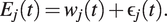 $$ {E}_j(t)={w}_j(t)+{\unicode{x025B}}_j(t). $$
Since $ {\unicode{x025B}}_j(t) $
is assumed to be pure noise, it does not carry relevant information, and
$ {\unicode{x025B}}_j(t) $
is assumed to be pure noise, it does not carry relevant information, and $ {w}_j(t) $
should be the part to focus on for monitoring purposes. To decompose
$ {w}_j(t) $
should be the part to focus on for monitoring purposes. To decompose $ {E}_j(t) $
into
$ {E}_j(t) $
into $ {w}_j(t) $
and
$ {w}_j(t) $
and $ {\unicode{x025B}}_j(t) $
, we use functional principal component analysis (FPCA). It is based on the Karhunen–Loeve expansion (Karhunen, Reference Karhunen1947; Loève, Reference Loève1946), which allows us to expand the random function
$ {\unicode{x025B}}_j(t) $
, we use functional principal component analysis (FPCA). It is based on the Karhunen–Loeve expansion (Karhunen, Reference Karhunen1947; Loève, Reference Loève1946), which allows us to expand the random function $ {E}_j(t) $
as
$ {E}_j(t) $
as
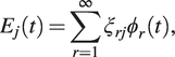 $$ {E}_j(t)=\sum \limits_{r=1}^{\infty }{\xi}_{rj}{\phi}_r(t), $$
where $ {\phi}_r $
are orthonormal eigenfunctions of the covariance, i.e.,
$ {\phi}_r $
are orthonormal eigenfunctions of the covariance, i.e., $ {\int}_{\mathcal{T}}{\phi}_r(t){\phi}_k(t) dt=1 $
if and only if
$ {\int}_{\mathcal{T}}{\phi}_r(t){\phi}_k(t) dt=1 $
if and only if $ k=r $
and zero otherwise. In particular, according to Mercer’s theorem (Mercer, Reference Mercer1909),
$ k=r $
and zero otherwise. In particular, according to Mercer’s theorem (Mercer, Reference Mercer1909),
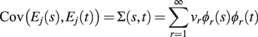 $$ \mathrm{Cov}\left({E}_j(s),{E}_j(t)\right)=\Sigma \left(s,t\right)=\sum \limits_{r=1}^{\infty }{\nu}_r{\phi}_r(s){\phi}_r(t) $$
with decreasing eigenvalues $ {\nu}_1\ge {\nu}_2\ge \dots \ge 0 $
. Furthermore,
$ {\nu}_1\ge {\nu}_2\ge \dots \ge 0 $
. Furthermore, $ {\xi}_{rj} $
are uncorrelated random scores with mean zero and variance
$ {\xi}_{rj} $
are uncorrelated random scores with mean zero and variance $ {\nu}_r $
,
$ {\nu}_r $
, $ r=1,2,\dots $
, and are independently normal if
$ r=1,2,\dots $
, and are independently normal if $ {E}_j $
is a Gaussian process.
$ {E}_j $
is a Gaussian process.
In FPCA, the sum in (3) is typically truncated at a finite upper limit $ m $
, which gives the best approximation of
$ m $
, which gives the best approximation of $ {E}_j $
with
$ {E}_j $
with $ m $
basis functions (Rice and Silverman, Reference Rice and Silverman1991). Looking at the fraction
$ m $
basis functions (Rice and Silverman, Reference Rice and Silverman1991). Looking at the fraction $ \left\{{\sum}_{r=1}^m{\nu}_r\right\}/\left\{{\sum}_{r=1}^{\infty }{\nu}_r\right\} $
allows a quantitative assessment of the variance explained by the approximation. For choosing the concrete value
$ \left\{{\sum}_{r=1}^m{\nu}_r\right\}/\left\{{\sum}_{r=1}^{\infty }{\nu}_r\right\} $
allows a quantitative assessment of the variance explained by the approximation. For choosing the concrete value $ m $
, there are various methods available (compare, e.g., Wang et al., Reference Wang, Chiou and Müller2016). One possibility is to use a value of
$ m $
, there are various methods available (compare, e.g., Wang et al., Reference Wang, Chiou and Müller2016). One possibility is to use a value of $ m $
such that a high proportion, e.g., 95% or 99%, of the overall variance is explained (e.g., Sørensen et al., Reference Sørensen, Goldsmith and Sangalli2013; Gertheiss et al., Reference Gertheiss, Rügamer, Liew and Greven2024), here we will use 99% throughout the paper. By choosing such a large value, it is reasonable to assume that the selected
$ m $
such that a high proportion, e.g., 95% or 99%, of the overall variance is explained (e.g., Sørensen et al., Reference Sørensen, Goldsmith and Sangalli2013; Gertheiss et al., Reference Gertheiss, Rügamer, Liew and Greven2024), here we will use 99% throughout the paper. By choosing such a large value, it is reasonable to assume that the selected $ m $
eigenfunctions account for all relevant features in the data, and the remainder is merely noise. Consequently, we set
$ m $
eigenfunctions account for all relevant features in the data, and the remainder is merely noise. Consequently, we set
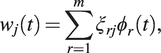 $$ {w}_j(t)=\sum \limits_{r=1}^m{\xi}_{rj}{\phi}_r(t), $$
and use the scores $ {\xi}_{1j},\dots, {\xi}_{mj} $
as damage-sensitive features for monitoring. As the functions
$ {\xi}_{1j},\dots, {\xi}_{mj} $
as damage-sensitive features for monitoring. As the functions $ \alpha, f,{\phi}_1,\dots, {\phi}_m $
are estimated from IC data in the model training phase, it is the scores obtained for future data that tell us whether the system outputs deviate from the values that would be expected for an IC structure over the day for given values of the covariate (and the specific time of the year, if
$ \alpha, f,{\phi}_1,\dots, {\phi}_m $
are estimated from IC data in the model training phase, it is the scores obtained for future data that tell us whether the system outputs deviate from the values that would be expected for an IC structure over the day for given values of the covariate (and the specific time of the year, if $ \alpha \left(t,{d}_j\right) $
instead of
$ \alpha \left(t,{d}_j\right) $
instead of $ \alpha (t) $
is used in model (1)). How to estimate the different model components, such as
$ \alpha (t) $
is used in model (1)). How to estimate the different model components, such as $ \alpha, f,{\phi}_1,\dots, {\phi}_m $
from the training data, and how to estimate the scores on future data, will be described in Section 2.2 below. At this point, it is important to note that if environmental and operational variables are present beyond
$ \alpha, f,{\phi}_1,\dots, {\phi}_m $
from the training data, and how to estimate the scores on future data, will be described in Section 2.2 below. At this point, it is important to note that if environmental and operational variables are present beyond $ z $
, and those variables are measured, model (1) can be extended to include multivariate covariates, see Section 2.4. If there are additional confounding effects that are not measured or not known at all, we can proceed analogously to the popular output-only method using (multivariate) PCA. That means we assume that the first, let us say,
$ z $
, and those variables are measured, model (1) can be extended to include multivariate covariates, see Section 2.4. If there are additional confounding effects that are not measured or not known at all, we can proceed analogously to the popular output-only method using (multivariate) PCA. That means we assume that the first, let us say, $ \rho $
components mainly account for variation induced by latent factors (Cross et al., Reference Cross, Manson, Worden and Pierce2012), so we only use the remaining scores
$ \rho $
components mainly account for variation induced by latent factors (Cross et al., Reference Cross, Manson, Worden and Pierce2012), so we only use the remaining scores $ {\xi}_{jr} $
,
$ {\xi}_{jr} $
, $ r>\rho $
, for monitoring. An important advantage of model (1) over output-only methods is that available covariate information can still be exploited through
$ r>\rho $
, for monitoring. An important advantage of model (1) over output-only methods is that available covariate information can still be exploited through $ f $
. How to modify our approach in terms of a pure output-only method if no covariate information is available at all will also be described in Section 2.4.
$ f $
. How to modify our approach in terms of a pure output-only method if no covariate information is available at all will also be described in Section 2.4.
2.2. Model training
Model fitting is carried out on in-control/Phase-I training data only. This will be described in Sections 2.2.1 and 2.2.2. In Section 2.2.3, we will discuss how to obtain the scores for Phase-II data that can be used for monitoring.
2.2.1. Basic model training strategy
For estimating functions such as $ \alpha $
or
$ \alpha $
or $ f $
in (1), we follow an approach popular in functional data analysis and semiparametric regression, compare Greven and Scheipl (Reference Greven and Scheipl2017) and Wood (Reference Wood2017). The unknown function, say
$ f $
in (1), we follow an approach popular in functional data analysis and semiparametric regression, compare Greven and Scheipl (Reference Greven and Scheipl2017) and Wood (Reference Wood2017). The unknown function, say $ f $
, is expanded in basis functions such that
$ f $
, is expanded in basis functions such that
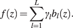 $$ f(z)=\sum \limits_{l=1}^L{\gamma}_l{b}_l(z). $$
A popular choice for $ {b}_1(z),\dots, {b}_L(z) $
is a cubic B-spline basis, which means that
$ {b}_1(z),\dots, {b}_L(z) $
is a cubic B-spline basis, which means that $ f $
is a cubic spline function (de Boor, Reference de Boor1978; Dierckx, Reference Dierckx1993). For being sufficiently flexible with respect to the types of functions that can be fitted through (6), typically, a rich basis with a large
$ f $
is a cubic spline function (de Boor, Reference de Boor1978; Dierckx, Reference Dierckx1993). For being sufficiently flexible with respect to the types of functions that can be fitted through (6), typically, a rich basis with a large $ L $
is chosen. A large
$ L $
is chosen. A large $ L $
, however, often leads to wiggly estimated functions if the basis coefficients
$ L $
, however, often leads to wiggly estimated functions if the basis coefficients $ {\gamma}_1,\dots, {\gamma}_L $
are fit without any smoothness constraint. The latter is typically imposed by adding a so-called penalty term when fitting the unknown coefficients through least-squares or maximum likelihood. A popular penalty is the integrated squared second derivative
$ {\gamma}_1,\dots, {\gamma}_L $
are fit without any smoothness constraint. The latter is typically imposed by adding a so-called penalty term when fitting the unknown coefficients through least-squares or maximum likelihood. A popular penalty is the integrated squared second derivative $ {\int}_{\mathcal{D}}{\left[{f^{\prime}}^{\prime }(z)\right]}^2 dz $
, where
$ {\int}_{\mathcal{D}}{\left[{f^{\prime}}^{\prime }(z)\right]}^2 dz $
, where $ \mathcal{D} $
is the domain of
$ \mathcal{D} $
is the domain of $ f $
. An alternative is a (quadratic) penalty on the discrete second- or third-order differences of the basis coefficients
$ f $
. An alternative is a (quadratic) penalty on the discrete second- or third-order differences of the basis coefficients $ {\gamma}_l $
, which gives a so-called P-spline, see Eilers and Marx (Reference Eilers and Marx1996) for details. If we assume that the eigenfunctions
$ {\gamma}_l $
, which gives a so-called P-spline, see Eilers and Marx (Reference Eilers and Marx1996) for details. If we assume that the eigenfunctions $ {\phi}_1,\dots, {\phi}_m $
from (5) are known, model (1) becomes
$ {\phi}_1,\dots, {\phi}_m $
from (5) are known, model (1) becomes
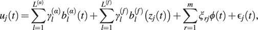 $$ {u}_j(t)=\sum \limits_{l=1}^{L^{\left(\alpha \right)}}{\gamma}_l^{\left(\alpha \right)}{b}_l^{\left(\alpha \right)}(t)+\sum \limits_{l=1}^{L^{(f)}}{\gamma}_l^{(f)}{b}_l^{(f)}\left({z}_j(t)\right)+\sum \limits_{r=1}^m{\xi}_{rj}\phi (t)+{\unicode{x025B}}_j(t), $$
where $ {\gamma}_l^{\left(\alpha \right)} $
,
$ {\gamma}_l^{\left(\alpha \right)} $
, $ {b}_l^{\left(\alpha \right)} $
,
$ {b}_l^{\left(\alpha \right)} $
, $ {\gamma}_l^{(f)} $
, and
$ {\gamma}_l^{(f)} $
, and $ {b}_l^{(f)} $
are the basis coefficients and basis functions for
$ {b}_l^{(f)} $
are the basis coefficients and basis functions for $ \alpha $
and
$ \alpha $
and $ f $
, respectively, and
$ f $
, respectively, and $ {\xi}_{rj} $
are day-specific random effects. Given a training dataset of system outputs and covariate information
$ {\xi}_{rj} $
are day-specific random effects. Given a training dataset of system outputs and covariate information $ \left\{{u}_j\left({t}_{ji}\right),{z}_j\left({t}_{ji}\right)\right\} $
for days
$ \left\{{u}_j\left({t}_{ji}\right),{z}_j\left({t}_{ji}\right)\right\} $
for days $ j=1,\dots, J $
and time points
$ j=1,\dots, J $
and time points $ {t}_{ji}\in \mathcal{T} $
,
$ {t}_{ji}\in \mathcal{T} $
, $ i=1,\dots, {N}_j $
, the unknown parameters
$ i=1,\dots, {N}_j $
, the unknown parameters $ {\gamma}_l^{\left(\alpha \right)},{\gamma}_l^{(f)} $
can be estimated through penalized least-squares, whereas the random effects
$ {\gamma}_l^{\left(\alpha \right)},{\gamma}_l^{(f)} $
can be estimated through penalized least-squares, whereas the random effects $ {\xi}_{rj} $
can be predicted using (linear) mixed models approaches. Specifying
$ {\xi}_{rj} $
can be predicted using (linear) mixed models approaches. Specifying $ {\xi}_{rj} $
as random effects makes this part of the model robust against over-fitting, thanks to the implicit shrinkage of random effects; compare, e.g., Fahrmeir et al. (Reference Fahrmeir, Kneib, Lang and Marx2013). The trade-off between model complexity concerning
$ {\xi}_{rj} $
as random effects makes this part of the model robust against over-fitting, thanks to the implicit shrinkage of random effects; compare, e.g., Fahrmeir et al. (Reference Fahrmeir, Kneib, Lang and Marx2013). The trade-off between model complexity concerning $ \alpha $
and
$ \alpha $
and $ f $
and fit to the data is controlled through the strength of the penalty on
$ f $
and fit to the data is controlled through the strength of the penalty on $ \alpha $
and
$ \alpha $
and $ f $
. Instead of using a penalty, model complexity could also be controlled through the number of basis functions
$ f $
. Instead of using a penalty, model complexity could also be controlled through the number of basis functions $ {L}^{\left(\alpha \right)} $
and
$ {L}^{\left(\alpha \right)} $
and $ {L}^{(f)} $
, but using a penalty makes the method robust against the concrete choice of
$ {L}^{(f)} $
, but using a penalty makes the method robust against the concrete choice of $ {L}^{\left(\alpha \right)} $
and
$ {L}^{\left(\alpha \right)} $
and $ {L}^{(f)} $
as it allows using large numbers (e.g., around 20), while controlling model complexity through smoothing; compare, e.g., Gertheiss et al. (Reference Gertheiss, Rügamer, Liew and Greven2024) and Wood (Reference Wood2017). There are a couple of options for choosing the strength of the penalty in a specific application, such as (generalized) cross-validation. In our case, the quadratic penalties used can also be incorporated into the mixed model framework, such that the strength of the penalty can be determined through (restricted) maximum likelihood, analogously to the variance components
$ {L}^{(f)} $
as it allows using large numbers (e.g., around 20), while controlling model complexity through smoothing; compare, e.g., Gertheiss et al. (Reference Gertheiss, Rügamer, Liew and Greven2024) and Wood (Reference Wood2017). There are a couple of options for choosing the strength of the penalty in a specific application, such as (generalized) cross-validation. In our case, the quadratic penalties used can also be incorporated into the mixed model framework, such that the strength of the penalty can be determined through (restricted) maximum likelihood, analogously to the variance components $ {\nu}_1,\dots, {\nu}_m $
and
$ {\nu}_1,\dots, {\nu}_m $
and $ {\sigma}^2 $
, see Wood (Reference Wood2011) and Wood (Reference Wood2017) for details. An in-depth discussion of these methods is beyond the scope of this paper. However, an important point to note is that model (1) and hence (7) is not identifiable in this general form given above because we may simply add some constant
$ {\sigma}^2 $
, see Wood (Reference Wood2011) and Wood (Reference Wood2017) for details. An in-depth discussion of these methods is beyond the scope of this paper. However, an important point to note is that model (1) and hence (7) is not identifiable in this general form given above because we may simply add some constant $ c $
to
$ c $
to $ \alpha $
while at the same time subtracting
$ \alpha $
while at the same time subtracting $ c $
from
$ c $
from $ f $
. Then, the two models are equivalent. In other words,
$ f $
. Then, the two models are equivalent. In other words, $ \alpha $
and
$ \alpha $
and $ f $
are only identifiable up to vertical shifts. That is why an overall constant
$ f $
are only identifiable up to vertical shifts. That is why an overall constant $ {\alpha}_0 $
is typically introduced in terms of
$ {\alpha}_0 $
is typically introduced in terms of
 $$ {u}_j(t)={\alpha}_0+\tilde{\alpha}(t)+f\left({z}_j(t)\right)+{E}_j(t), $$
and $ \tilde{\alpha} $
and
$ \tilde{\alpha} $
and $ f $
are centered in some sense. The constraint used in the R package mgcv (Wood, Reference Wood2017), which we use here for model training, is
$ f $
are centered in some sense. The constraint used in the R package mgcv (Wood, Reference Wood2017), which we use here for model training, is $ {\sum}_{i,j}\tilde{\alpha}\left({t}_{ji}\right)=0\hskip0.35em \mathrm{and}\hskip0.35em {\sum}_{i,j}f\left({z}_j\left({t}_{ji}\right)\right)=0 $
, respectively. Furthermore, it is worth noting that measurement points
$ {\sum}_{i,j}\tilde{\alpha}\left({t}_{ji}\right)=0\hskip0.35em \mathrm{and}\hskip0.35em {\sum}_{i,j}f\left({z}_j\left({t}_{ji}\right)\right)=0 $
, respectively. Furthermore, it is worth noting that measurement points $ {t}_{ji} $
neither need to be the same for each day nor on a regular grid. As a consequence, missing values in the output profiles or the covariate curves are allowed.
$ {t}_{ji} $
neither need to be the same for each day nor on a regular grid. As a consequence, missing values in the output profiles or the covariate curves are allowed.
2.2.2. Estimation of eigenfunctions
In Section 2.2.1, we assumed that the eigenfunctions $ {\phi}_r $
,
$ {\phi}_r $
, $ r=1,\dots, m $
, are known. In practice, those functions need to be estimated from the training data in some way. To do so, we first fit model (1), or a modification from below, with a working independence assumption concerning
$ r=1,\dots, m $
, are known. In practice, those functions need to be estimated from the training data in some way. To do so, we first fit model (1), or a modification from below, with a working independence assumption concerning $ {E}_j(t) $
(Scheipl et al., Reference Scheipl, Staicu and Greven2015). Specifically, this means that
$ {E}_j(t) $
(Scheipl et al., Reference Scheipl, Staicu and Greven2015). Specifically, this means that $ {E}_j(t) $
from (1) is white noise and
$ {E}_j(t) $
from (1) is white noise and $ {w}_j(t) $
from (2) is omitted; compare, e.g., Ivanescu et al. (Reference Ivanescu, Staicu, Scheipl and Greven2015). Then, we use the resulting estimates of the error process for FPCA, plug in the estimated eigenfunctions
$ {w}_j(t) $
from (2) is omitted; compare, e.g., Ivanescu et al. (Reference Ivanescu, Staicu, Scheipl and Greven2015). Then, we use the resulting estimates of the error process for FPCA, plug in the estimated eigenfunctions $ {\hat{\phi}}_r $
, and fit the final model as discussed above. Such a two-step approach has worked well in the past (Gertheiss et al., Reference Gertheiss, Goldsmith and Staicu2017). For FPCA, we use an approach based on Yao et al. (Reference Yao, Müller and Wang2005) that accommodates functions with additional white noise errors and thus works relatively generally (Gertheiss et al., Reference Gertheiss, Rügamer, Liew and Greven2024). The idea is to incorporate smoothing into estimating the covariance in (4). The estimation is based on the cross-products of observed points within error curves,
$ {\hat{\phi}}_r $
, and fit the final model as discussed above. Such a two-step approach has worked well in the past (Gertheiss et al., Reference Gertheiss, Goldsmith and Staicu2017). For FPCA, we use an approach based on Yao et al. (Reference Yao, Müller and Wang2005) that accommodates functions with additional white noise errors and thus works relatively generally (Gertheiss et al., Reference Gertheiss, Rügamer, Liew and Greven2024). The idea is to incorporate smoothing into estimating the covariance in (4). The estimation is based on the cross-products of observed points within error curves, $ {E}_j\left({t}_{ji}\right){E}_j\left({t}_{j{i}^{\prime }}\right) $
, which are rough estimates of
$ {E}_j\left({t}_{ji}\right){E}_j\left({t}_{j{i}^{\prime }}\right) $
, which are rough estimates of $ Cov\left(E\left({t}_{ji}\right),E\left({t}_{j{i}^{\prime }}\right)\right) $
. All cross-products are pooled, and a smoothing method of choice is used for bivariate smoothing. Yao et al. (Reference Yao, Müller and Wang2005) used local polynomial smoothing, while the refund R package (Goldsmith et al., Reference Goldsmith, Scheipl, Huang, Wrobel, Di, Gellar, Harezlak, McLean, Swihart, Xiao, Crainiceanu and Reiss2022) used here employs penalized splines. If an additional white noise error is assumed (as we do here), the diagonal cross-products approximate the variance of the structural component plus the error variance. The diagonal is thus left out for smoothing. Once the smooth covariance is available, the orthogonal decomposition (4) is done numerically on a fine grid using the usual matrix eigendecomposition.
$ Cov\left(E\left({t}_{ji}\right),E\left({t}_{j{i}^{\prime }}\right)\right) $
. All cross-products are pooled, and a smoothing method of choice is used for bivariate smoothing. Yao et al. (Reference Yao, Müller and Wang2005) used local polynomial smoothing, while the refund R package (Goldsmith et al., Reference Goldsmith, Scheipl, Huang, Wrobel, Di, Gellar, Harezlak, McLean, Swihart, Xiao, Crainiceanu and Reiss2022) used here employs penalized splines. If an additional white noise error is assumed (as we do here), the diagonal cross-products approximate the variance of the structural component plus the error variance. The diagonal is thus left out for smoothing. Once the smooth covariance is available, the orthogonal decomposition (4) is done numerically on a fine grid using the usual matrix eigendecomposition.
The entire model training workflow is summarized in the orange part of Figure 2. We first use the Phase-I data (step 0) to fit the initial model with working independence in step 1. On the resulting residuals, the “observed” error process, we carry out FPCA to obtain estimates of the eigenfunctions (step 2). For choosing the number of components, we use the usual threshold of 95% or 99% of the variance explained. Then, the eigenfunctions are used to train the final model in step 3. From this model, we obtain estimates of the fixed and random effects, the variance components, and the residuals. Particularly, the fixed effects, the eigenfunctions, and the variance components will be needed to estimate Phase-II component scores and implement a monitoring scheme as described below.
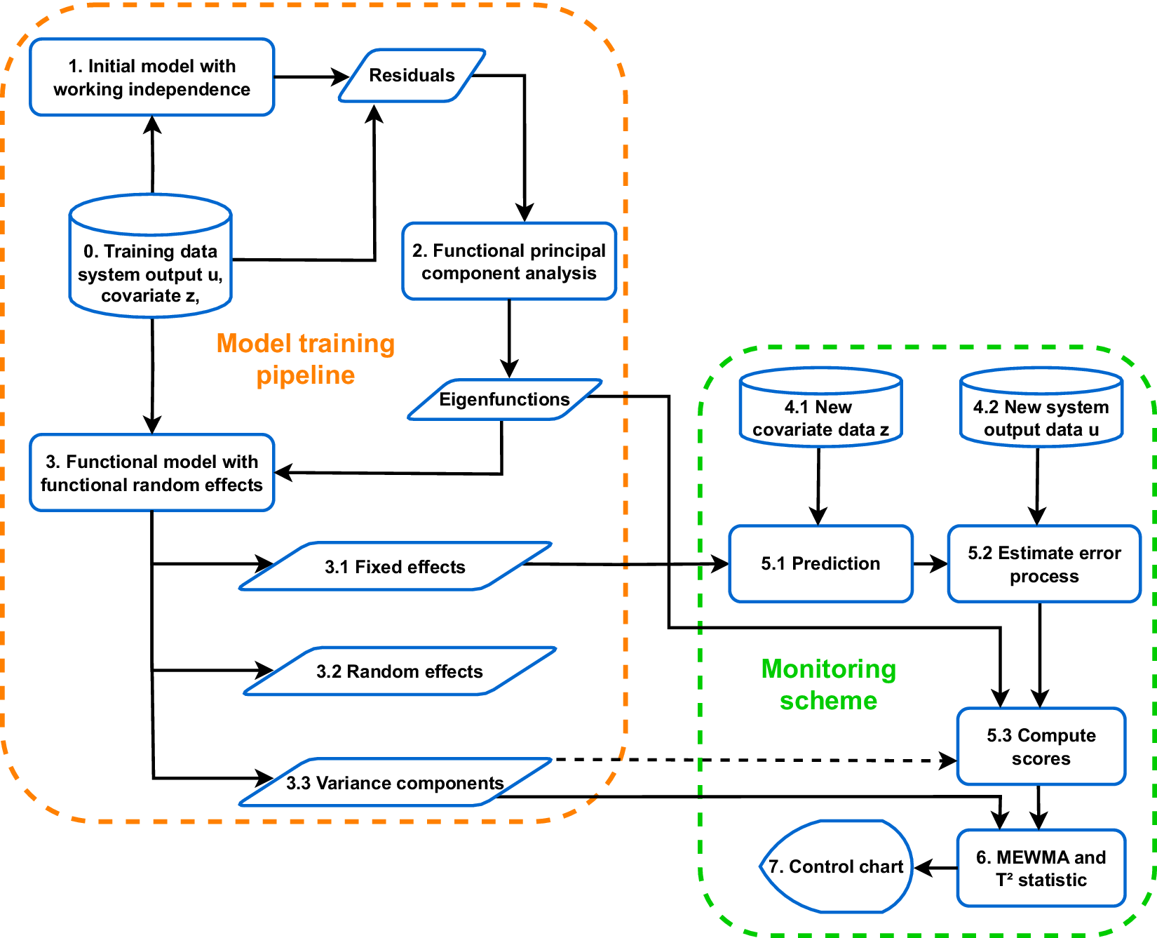
Figure 2. Visual summary of the CAFDA-SHM framework.
2.2.3. Estimation of phase-II scores
Once the mixed model for function-on-function regression has been trained, it can be used to monitor future system outputs if the covariates in the trained model are available as well. The corresponding data is denoted as “new covariate data $ z $
” and “new system output data
$ z $
” and “new system output data $ u $
” in Figure 2. An essential input for the monitoring scheme described in the next subsection are the principal component scores
$ u $
” in Figure 2. An essential input for the monitoring scheme described in the next subsection are the principal component scores $ {\xi}_{1,g},\dots, {\xi}_{m,g} $
for a new day
$ {\xi}_{1,g},\dots, {\xi}_{m,g} $
for a new day $ g $
in Phase II. To estimate those scores from the new data, we first use the fixed effects from the Phase-I model,
$ g $
in Phase II. To estimate those scores from the new data, we first use the fixed effects from the Phase-I model, $ \hat{\alpha}\left({t}_{gi}\right) $
and
$ \hat{\alpha}\left({t}_{gi}\right) $
and $ \hat{f}\left({z}_g\left({t}_{gi}\right)\right) $
from (1), to obtain a prediction for the system outputs
$ \hat{f}\left({z}_g\left({t}_{gi}\right)\right) $
from (1), to obtain a prediction for the system outputs $ {u}_g\left({t}_{gi}\right) $
. Here,
$ {u}_g\left({t}_{gi}\right) $
. Here, $ {t}_{gi} $
,
$ {t}_{gi} $
, $ i=1,\dots, {N}_g $
, denote the time instances of the covariate
$ i=1,\dots, {N}_g $
, denote the time instances of the covariate $ {z}_g\left({t}_{gi}\right) $
available at day
$ {z}_g\left({t}_{gi}\right) $
available at day $ g $
. Then, those predictions are subtracted from the actually observed
$ g $
. Then, those predictions are subtracted from the actually observed $ {u}_g\left({t}_{gi}\right) $
to obtain estimated measurements
$ {u}_g\left({t}_{gi}\right) $
to obtain estimated measurements $ {\hat{E}}_g\left({t}_{gi}\right) $
of the error process. If those time points are sufficiently dense over the course of day
$ {\hat{E}}_g\left({t}_{gi}\right) $
of the error process. If those time points are sufficiently dense over the course of day $ g $
, which is typically the case if day
$ g $
, which is typically the case if day $ g $
is (nearly) over, the scores can be estimated through numerical integration such that
$ g $
is (nearly) over, the scores can be estimated through numerical integration such that
 $$ {\hat{\xi}}_{r,g}={\int}_{\mathcal{T}}{\hat{E}}_g(t){\hat{\phi}}_r(t) dt. $$
However, sometimes there is a substantial amount of missing values in the $ u $
or
$ u $
or $ z $
data, e.g., due to technical problems, or — more importantly — the score estimates have to be available before the new day is over. In the latter case, we may say that all the data points after some time point are “missing.” In both situations, the interpretation as a mixed model is helpful, as this also allows for predicting the random effects for a reduced set of measurement points
$ z $
data, e.g., due to technical problems, or — more importantly — the score estimates have to be available before the new day is over. In the latter case, we may say that all the data points after some time point are “missing.” In both situations, the interpretation as a mixed model is helpful, as this also allows for predicting the random effects for a reduced set of measurement points $ {t}_{gi} $
.
$ {t}_{gi} $
.
For that purpose, let $ {\boldsymbol{\phi}}_{gr}={({\phi}_r({t}_{g1}),\dots, {\phi}_r({t}_{g{N}_g}))}^{\mathrm{T}} $
be the
$ {\boldsymbol{\phi}}_{gr}={({\phi}_r({t}_{g1}),\dots, {\phi}_r({t}_{g{N}_g}))}^{\mathrm{T}} $
be the $ r $
th eigenfunction evaluated at time points
$ r $
th eigenfunction evaluated at time points $ {t}_{gi} $
,
$ {t}_{gi} $
, $ i=1,\dots, {N}_g $
,
$ i=1,\dots, {N}_g $
, $ r=1,\dots, m $
, and
$ r=1,\dots, m $
, and $ {\Sigma}_{{\mathbf{E}}_g} $
the covariance matrix of the error vector
$ {\Sigma}_{{\mathbf{E}}_g} $
the covariance matrix of the error vector $ {\mathbf{E}}_g={\left({E}_g\left({t}_{g1}\right),\dots, {E}_g\left({t}_{gN_g}\right)\right)}^{\mathrm{T}} $
. Then, assuming a Gaussian distribution, the conditional expectation of the score
$ {\mathbf{E}}_g={\left({E}_g\left({t}_{g1}\right),\dots, {E}_g\left({t}_{gN_g}\right)\right)}^{\mathrm{T}} $
. Then, assuming a Gaussian distribution, the conditional expectation of the score $ {\xi}_{r,g} $
given
$ {\xi}_{r,g} $
given $ {\mathbf{E}}_g $
is
$ {\mathbf{E}}_g $
is $ \unicode{x1D53C}\left({\xi}_{r,g}|{\mathbf{E}}_g\right)={\nu}_r{\boldsymbol{\phi}}_{gr}^{\mathrm{T}}{\Sigma}_{{\mathbf{E}}_g}^{-1}{\mathbf{E}}_g,r=1,\dots, m $
(Yao et al., Reference Yao, Müller and Wang2005). Due to (2) and (5), the matrix
$ \unicode{x1D53C}\left({\xi}_{r,g}|{\mathbf{E}}_g\right)={\nu}_r{\boldsymbol{\phi}}_{gr}^{\mathrm{T}}{\Sigma}_{{\mathbf{E}}_g}^{-1}{\mathbf{E}}_g,r=1,\dots, m $
(Yao et al., Reference Yao, Müller and Wang2005). Due to (2) and (5), the matrix $ {\Sigma}_{{\mathbf{E}}_g} $
can be estimated as
$ {\Sigma}_{{\mathbf{E}}_g} $
can be estimated as $ {\hat{\Sigma}}_{{\mathbf{E}}_g}={\hat{\boldsymbol{\Phi}}}_g\hskip0.1em \mathrm{diag}\hskip0.1em ({\hat{\nu}}_1,\dots, {\hat{\nu}}_m){\hat{\boldsymbol{\Phi}}}_g^{\mathrm{T}}+{\hat{\sigma}}^2{\mathbf{I}}_{N_g} $
, with
$ {\hat{\Sigma}}_{{\mathbf{E}}_g}={\hat{\boldsymbol{\Phi}}}_g\hskip0.1em \mathrm{diag}\hskip0.1em ({\hat{\nu}}_1,\dots, {\hat{\nu}}_m){\hat{\boldsymbol{\Phi}}}_g^{\mathrm{T}}+{\hat{\sigma}}^2{\mathbf{I}}_{N_g} $
, with $ {\hat{\boldsymbol{\Phi}}}_g=({\hat{\boldsymbol{\phi}}}_{g1}|\dots |{\hat{\boldsymbol{\phi}}}_{gm}) $
. After plugging in the estimates
$ {\hat{\boldsymbol{\Phi}}}_g=({\hat{\boldsymbol{\phi}}}_{g1}|\dots |{\hat{\boldsymbol{\phi}}}_{gm}) $
. After plugging in the estimates $ {\hat{\sigma}}^2 $
,
$ {\hat{\sigma}}^2 $
, $ {\hat{\nu}}_r $
,
$ {\hat{\nu}}_r $
, $ {\hat{\phi}}_r $
,
$ {\hat{\phi}}_r $
, $ r=1,\dots, m $
, from the model training phase and
$ r=1,\dots, m $
, from the model training phase and $ {\hat{\mathbf{E}}}_g={\left({\hat{E}}_g\left({t}_{g1}\right),\dots, {\hat{E}}_g\left({t}_{gN_g}\right)\right)}^{\mathrm{T}} $
from above, we obtain the estimated scores
$ {\hat{\mathbf{E}}}_g={\left({\hat{E}}_g\left({t}_{g1}\right),\dots, {\hat{E}}_g\left({t}_{gN_g}\right)\right)}^{\mathrm{T}} $
from above, we obtain the estimated scores
 $$ {\hat{\xi}}_{r,g}={\hat{\nu}}_r{\hat{\boldsymbol{\phi}}}_{gr}^{\mathrm{T}}{\hat{\Sigma}}_{{\mathbf{E}}_g}^{-1}{\hat{\mathbf{E}}}_g,\hskip0.35em r=1,\dots, m. $$
These scores can then be used as input to a control chart. The workflow of estimating Phase-II scores is also summarized in Figure 2 (steps 4.1–5.3). The dashed arrow towards the scores (5.3 in Figure 2) indicates that variance components $ {\hat{\nu}}_1,\dots, {\hat{\nu}}_m $
and
$ {\hat{\nu}}_1,\dots, {\hat{\nu}}_m $
and $ {\hat{\sigma}}^2 $
are needed if using (10) but not for (9).
$ {\hat{\sigma}}^2 $
are needed if using (10) but not for (9).
2.3. Control charts
After accounting for environmental influences through appropriate modeling, the system outputs can be monitored by applying a control chart. A multivariate Hotelling control chart is often used to quickly detect a shift in the structural condition (Deraemaeker et al., Reference Deraemaeker, Reynders, De Roeck and Kullaa2008; Magalhães et al., Reference Magalhães, Cunha and Caetano2012; Comanducci et al., Reference Comanducci, Magalhães, Ubertini and Cunha2016). Here, we employ a memory-type control chart, the Multivariate Exponentially Weighted Moving Average (MEWMA) introduced by Lowry et al. (Reference Lowry, Woodall, Champ and Rigdon1992) to the Phase-II scores $ {\xi}_{1,g},\dots, {\xi}_{m,g} $
,
$ {\xi}_{1,g},\dots, {\xi}_{m,g} $
, $ g=1,2,\dots $
, from Section 2.2.3. The MEWMA contains the Hotelling chart as a special case. The MEWMA chart assumes serially independent, normally distributed vectors
$ g=1,2,\dots $
, from Section 2.2.3. The MEWMA contains the Hotelling chart as a special case. The MEWMA chart assumes serially independent, normally distributed vectors $ {\boldsymbol{\xi}}_1,{\boldsymbol{\xi}}_2,\dots $
of dimension
$ {\boldsymbol{\xi}}_1,{\boldsymbol{\xi}}_2,\dots $
of dimension $ m $
with
$ m $
with $ {\boldsymbol{\xi}}_g\sim \mathcal{N}(\boldsymbol{\mu}, \boldsymbol{\Lambda} ) $
. We follow Knoth (Reference Knoth2017) and define a mean vector
$ {\boldsymbol{\xi}}_g\sim \mathcal{N}(\boldsymbol{\mu}, \boldsymbol{\Lambda} ) $
. We follow Knoth (Reference Knoth2017) and define a mean vector $ \boldsymbol{\mu} $
that follows a change point model
$ \boldsymbol{\mu} $
that follows a change point model $ \boldsymbol{\mu} ={\boldsymbol{\mu}}_0 $
for
$ \boldsymbol{\mu} ={\boldsymbol{\mu}}_0 $
for $ g<\tau $
and
$ g<\tau $
and $ \boldsymbol{\mu} ={\boldsymbol{\mu}}_1 $
for
$ \boldsymbol{\mu} ={\boldsymbol{\mu}}_1 $
for $ g\ge \tau $
for an unknown time point
$ g\ge \tau $
for an unknown time point $ \tau $
and by definition
$ \tau $
and by definition $ {\boldsymbol{\mu}}_0=\mathbf{0} $
, see Section 2.1. For in-control data, the scores
$ {\boldsymbol{\mu}}_0=\mathbf{0} $
, see Section 2.1. For in-control data, the scores $ {\xi}_{1,g},\dots, {\xi}_{m,g} $
are assumed to be uncorrelated with variances
$ {\xi}_{1,g},\dots, {\xi}_{m,g} $
are assumed to be uncorrelated with variances $ {\nu}_1,\dots, {\nu}_m $
, see also Section 2.1. Hence, the covariance matrix
$ {\nu}_1,\dots, {\nu}_m $
, see also Section 2.1. Hence, the covariance matrix $ \boldsymbol{\Lambda} $
is diagonal with
$ \boldsymbol{\Lambda} $
is diagonal with $ \boldsymbol{\Lambda} =\mathrm{diag}({\nu}_1,\dots, {\nu}_m) $
. Then, we apply the following smoothing procedure to compute the MEWMA statistic (step 6 in Figure 2)
$ \boldsymbol{\Lambda} =\mathrm{diag}({\nu}_1,\dots, {\nu}_m) $
. Then, we apply the following smoothing procedure to compute the MEWMA statistic (step 6 in Figure 2)
 $$ {\boldsymbol{\omega}}_g=\left(1-\lambda \right){\boldsymbol{\omega}}_{g-1}+\lambda {\hat{\boldsymbol{\xi}}}_g,\hskip1em {\boldsymbol{\omega}}_0=\mathbf{0} $$
with $ g=1,2,\dots $
, smoothing constant
$ g=1,2,\dots $
, smoothing constant $ 0<\lambda \le 1 $
, and the estimated scores
$ 0<\lambda \le 1 $
, and the estimated scores $ {\hat{\xi}}_{r,g} $
from (9) or (10) collected in
$ {\hat{\xi}}_{r,g} $
from (9) or (10) collected in $ {\hat{\boldsymbol{\xi}}}_g $
such that
$ {\hat{\boldsymbol{\xi}}}_g $
such that $ {\hat{\boldsymbol{\xi}}}_g={\left({\hat{\xi}}_{1,g},\dots, {\hat{\xi}}_{m,g}\right)}^{\mathrm{T}} $
. The smoothing parameter
$ {\hat{\boldsymbol{\xi}}}_g={\left({\hat{\xi}}_{1,g},\dots, {\hat{\xi}}_{m,g}\right)}^{\mathrm{T}} $
. The smoothing parameter $ \lambda $
controls the sensitivity of the shift to be detected. Smaller values of
$ \lambda $
controls the sensitivity of the shift to be detected. Smaller values of $ \lambda $
such as
$ \lambda $
such as $ \lambda \in \left\{\mathrm{0.1,0.2,0.3}\right\} $
, are usually selected to detect smaller shifts (Hunter, Reference Hunter1986), while
$ \lambda \in \left\{\mathrm{0.1,0.2,0.3}\right\} $
, are usually selected to detect smaller shifts (Hunter, Reference Hunter1986), while $ \lambda =1 $
results in the Hotelling chart. In this study, we use
$ \lambda =1 $
results in the Hotelling chart. In this study, we use $ \lambda =0.3 $
. The control statistic is the Mahalanobis distance
$ \lambda =0.3 $
. The control statistic is the Mahalanobis distance
 $$ {T}_g^2={({\boldsymbol{\omega}}_g-{\boldsymbol{\mu}}_0)}^{\mathrm{T}}{\boldsymbol{\Lambda}}_{\boldsymbol{\omega}}^{-1}({\boldsymbol{\omega}}_g-{\boldsymbol{\mu}}_0), $$
with an asymptotic covariance matrix of $ {\boldsymbol{\omega}}_g $
,
$ {\boldsymbol{\omega}}_g $
, $ {\boldsymbol{\Lambda}}_{\boldsymbol{\omega}}={\lim}_{g\to \mathrm{\infty}}\mathrm{C}\mathrm{o}\mathrm{v}({\boldsymbol{\omega}}_g)=\{\frac{\lambda }{2-\lambda}\}\boldsymbol{\Lambda} $
. Note, if the scores in
$ {\boldsymbol{\Lambda}}_{\boldsymbol{\omega}}={\lim}_{g\to \mathrm{\infty}}\mathrm{C}\mathrm{o}\mathrm{v}({\boldsymbol{\omega}}_g)=\{\frac{\lambda }{2-\lambda}\}\boldsymbol{\Lambda} $
. Note, if the scores in $ {\hat{\boldsymbol{\xi}}}_g $
are estimated on a reduced set of measurement points (e.g., due to missing values), the model-based estimates
$ {\hat{\boldsymbol{\xi}}}_g $
are estimated on a reduced set of measurement points (e.g., due to missing values), the model-based estimates $ {\hat{\nu}}_1,\dots, {\hat{\nu}}_m $
(step 3.3 in Figure 2) may not give the correct variances of the scores. In a case like this, it is recommended to run steps 5.1–5.3 from Figure 2 on the training data but with the reduced set of measurement points to obtain adjusted estimates of the variances (through the empirical versions), which can then be used in
$ {\hat{\nu}}_1,\dots, {\hat{\nu}}_m $
(step 3.3 in Figure 2) may not give the correct variances of the scores. In a case like this, it is recommended to run steps 5.1–5.3 from Figure 2 on the training data but with the reduced set of measurement points to obtain adjusted estimates of the variances (through the empirical versions), which can then be used in $ \boldsymbol{\Lambda} $
.
$ \boldsymbol{\Lambda} $
.
The MEWMA chart issues an alarm if $ {T}_i^2>{h}_4 $
, i.e., the control statistic is above the threshold value
$ {T}_i^2>{h}_4 $
, i.e., the control statistic is above the threshold value $ {h}_4 $
. The stopping time
$ {h}_4 $
. The stopping time $ N=\mathrm{min}\{g\ge 1:{T}_g^2>{h}_4\} $
, also known as average run length (ARL), is often used to measure the control chart’s performance. It is defined as the average number of observations until the chart signals an alarm. If the process is in-control, the ARL (ARL
$ N=\mathrm{min}\{g\ge 1:{T}_g^2>{h}_4\} $
, also known as average run length (ARL), is often used to measure the control chart’s performance. It is defined as the average number of observations until the chart signals an alarm. If the process is in-control, the ARL (ARL $ {}_0 $
) should be high to avoid false alarms. If there is a change in the underlying process, the ARL (ARL
$ {}_0 $
) should be high to avoid false alarms. If there is a change in the underlying process, the ARL (ARL $ {}_1 $
) should be low to detect changes quickly. To determine the threshold value, the ARL must be calculated when the process is in-control, usually applying a grid search or a secant rule. This ARL
$ {}_1 $
) should be low to detect changes quickly. To determine the threshold value, the ARL must be calculated when the process is in-control, usually applying a grid search or a secant rule. This ARL $ {}_0 $
can be calculated as described in Knoth (Reference Knoth2017) and is implemented in R package spc (Knoth, Reference Knoth2022). An evaluation of our CAFDA framework on artificial data is demonstrated in Section 3.
$ {}_0 $
can be calculated as described in Knoth (Reference Knoth2017) and is implemented in R package spc (Knoth, Reference Knoth2022). An evaluation of our CAFDA framework on artificial data is demonstrated in Section 3.
2.4. Modified and extended models
Our basic model (1) is a particular case of a functional additive mixed model, as introduced and discussed by Scheipl et al. (Reference Scheipl, Staicu and Greven2015), Scheipl et al. (Reference Scheipl, Gertheiss and Greven2016), and Greven and Scheipl (Reference Greven and Scheipl2017), which can be simplified, modified, or extended in various ways depending on the available data and prior knowledge. Some alternative specifications that may be an option with the data available in our case studies in Section 4 are recapped as follows.
-
• Standard linear models: If we have reason to believe that potential daily patterns can be explained entirely through variations in
$ z $
, we can replace
$ \alpha (t) $
with a constant
$ {\alpha}_0 $
. Similarly, if it is believed that the association of the confounder
$ z $
and system output
$ u $
is linear, we can replace
$ f\left({z}_j(t)\right) $
in (1) with
$ \beta {z}_j(t) $
. So, the standard linear regression model is a special case in our broader framework. Typically, if fitting the more flexible model (1) to the data, a nearly constant
$ \alpha $
and a close to linear
$ f $
will indicate that the simpler model is sufficient. -
• Unmeasured covariates: If covariate information is unavailable,
$ f\left({z}_j(t)\right) $
can be omitted, and our approach turns into an output-only method using FPCA. In that case, replacing
$ \alpha (t) $
with
$ \alpha \left(t,{d}_j\right) $
is highly recommended. The reason for this is that variables such as temperature typically vary over the day and year, imposing a specific yearly pattern on
$ u $
as well. The latter can be modeled through
$ \alpha \left(t,{d}_j\right) $
. -
• Multiple covariates: If
$ p $
covariates
$ {z}_{j1}(t),\dots, {z}_{jp}(t) $
, e.g., temperature, relative humidity, wind speed, solar radiation, have an effect, or if several temperature sensors are used to account for the local temperatures at different spatial locations in the construction material, their effects can be combined additively in (1) by replacing the term
$ f\left({z}_j(t)\right) $
with
$ {\sum}_{k=1}^p{f}_k\left({z}_{jk}(t)\right) $
. -
• Covariate interactions: If
$ {z}_{jk}(t),{z}_{jl}(t) $
are believed to have an interacting effect on the system output, e.g., temperature and relative humidity, model (1) can also contain (two-way) interactions in terms of
$ {f}_{kl}\left({z}_{jk}(t),{z}_{jl}(t)\right) $
. In theory, interactions of higher order are possible as well. However, it can be challenging to estimate the corresponding parameter functions due to the computing resources and amount of data needed to learn those interactions reliably, compare Section 2.2.


While all those models are so-called concurrent models, which are useful to adjust for the temperature of the structure itself, the framework of functional additive mixed models is flexible enough to cope with delayed effects (as, e.g., plausible for ambient temperature) using so-called historical functional effects (Scheipl et al., Reference Scheipl, Gertheiss and Greven2016). Also, the very popular linear function-on-function regression approach (Centofanti et al., Reference Centofanti, Lepore, Menafoglio, Palumbo and Vantini2021) is included as a special case. An overview of various modeling options beyond those discussed above is provided in Appendix A. The decision about the model to use should be based on subject matter knowledge, the available data, the goodness-of-fit, and the parameter estimates. As pointed out, concurrent models are particularly useful if the structure’s temperature is measured. If more than one (potential) confounder is measured, the model should be able to include multiple covariates. To distinguish between additive effects and interactions, the model fits should be compared, and the estimated (two-dimensional) surface $ {f}_{kl} $
should be inspected visually. The less complex (additive) model should be chosen if the two model fits are similar and the surface looks like two additive effects; see also Section 4.1. Sometimes, it may even be known from prior studies that a particular confounder effect is (almost) linear. In a case like this, however, choosing a more complex model like (1) is usually fine, too, because due to the penalty, the estimated
$ {f}_{kl} $
should be inspected visually. The less complex (additive) model should be chosen if the two model fits are similar and the surface looks like two additive effects; see also Section 4.1. Sometimes, it may even be known from prior studies that a particular confounder effect is (almost) linear. In a case like this, however, choosing a more complex model like (1) is usually fine, too, because due to the penalty, the estimated $ f $
will typically turn out to be (nearly) linear if the data point in that direction (compare Section 4.2).
$ f $
will typically turn out to be (nearly) linear if the data point in that direction (compare Section 4.2).
The resulting modifications concerning model fitting can be summarized as follows. If model (1) is simplified, parameterization (7) simplifies, as well. For instance, if an output-only approach based entirely on FPCA is used, the part in (7) referring to the regression function $ f $
vanishes. If the latter is assumed to be linear, only the corresponding
$ f $
vanishes. If the latter is assumed to be linear, only the corresponding $ \beta $
has to be estimated. If
$ \beta $
has to be estimated. If $ \beta $
is allowed to change over the course of the day in terms of
$ \beta $
is allowed to change over the course of the day in terms of $ \beta (t) $
, this function can be expanded in basis functions as it was done with
$ \beta (t) $
, this function can be expanded in basis functions as it was done with $ f $
in (6) and estimated analogously. If, on the other hand, multiple covariates are given, and model (1) is extended to
$ f $
in (6) and estimated analogously. If, on the other hand, multiple covariates are given, and model (1) is extended to $ {\sum}_{k=1}^p{f}_k\left({z}_{jk}(t)\right) $
instead of a single
$ {\sum}_{k=1}^p{f}_k\left({z}_{jk}(t)\right) $
instead of a single $ f\left({z}_j(t)\right) $
, we have to add basis representations
$ f\left({z}_j(t)\right) $
, we have to add basis representations $ {\sum}_{l_k=1}^{L^{\left({f}_k\right)}}{\gamma}_{l_k}^{\left({f}_k\right)}{b}_{l_k}^{\left({f}_k\right)}\left({z}_{jk}(t)\right) $
for each component
$ {\sum}_{l_k=1}^{L^{\left({f}_k\right)}}{\gamma}_{l_k}^{\left({f}_k\right)}{b}_{l_k}^{\left({f}_k\right)}\left({z}_{jk}(t)\right) $
for each component $ {f}_k $
,
$ {f}_k $
, $ k=1,\dots, p $
, in (7). If we want to account for both daily and yearly patterns in a purely additive way, that is,
$ k=1,\dots, p $
, in (7). If we want to account for both daily and yearly patterns in a purely additive way, that is, $ \alpha \left(t,{d}_j\right)={\alpha}_0+{\tilde{\alpha}}_1(t)+{\tilde{\alpha}}_2\left({d}_j\right) $
, the procedure is completely analogous. However, if
$ \alpha \left(t,{d}_j\right)={\alpha}_0+{\tilde{\alpha}}_1(t)+{\tilde{\alpha}}_2\left({d}_j\right) $
, the procedure is completely analogous. However, if $ \alpha \left(t,{d}_j\right) $
is supposed to be a surface, or if a two-way interaction, say
$ \alpha \left(t,{d}_j\right) $
is supposed to be a surface, or if a two-way interaction, say $ f\left({z}_{j1}(t),{z}_{j2}(t)\right) $
in (1), is to be fitted, some minor modifications are necessary. The unknown functions (
$ f\left({z}_{j1}(t),{z}_{j2}(t)\right) $
in (1), is to be fitted, some minor modifications are necessary. The unknown functions ( $ \alpha $
and
$ \alpha $
and $ f $
, respectively) now have two arguments, meaning that the basis needs to be chosen appropriately, e.g., as a so-called tensor product basis. For instance, if considering
$ f $
, respectively) now have two arguments, meaning that the basis needs to be chosen appropriately, e.g., as a so-called tensor product basis. For instance, if considering $ f $
, equation (6) turns into
$ f $
, equation (6) turns into
 $$ f\left({z}_1,{z}_2\right)=\sum \limits_{l_1=1}^{L_1}\sum \limits_{l_2=1}^{L_2}{\gamma}_{l_1,{l}_2}{b}_{l_1}\left({z}_1\right){b}_{l_2}\left({z}_2\right), $$
and smoothing is typically done in both the $ {z}_1 $
- and
$ {z}_1 $
- and $ {z}_2 $
-directions. Having said that, the model complexity increases in terms of the number of basis coefficients
$ {z}_2 $
-directions. Having said that, the model complexity increases in terms of the number of basis coefficients $ {\gamma}_{l_1,{l}_2} $
that need to be fitted. As pointed out earlier, higher-order interactions can also be estimated, but the number of coefficients increases even further. Bivariate (or even higher dimensional) smoothers allowing for terms such as (13) are available in mgcv, and corresponding estimates will be shown in the real-world data evaluations in Section 4. The approach for bivariate
$ {\gamma}_{l_1,{l}_2} $
that need to be fitted. As pointed out earlier, higher-order interactions can also be estimated, but the number of coefficients increases even further. Bivariate (or even higher dimensional) smoothers allowing for terms such as (13) are available in mgcv, and corresponding estimates will be shown in the real-world data evaluations in Section 4. The approach for bivariate $ \alpha \left(t,{d}_j\right) $
or
$ \alpha \left(t,{d}_j\right) $
or $ f\left({z}_j(t),t\right) $
cases, where the potentially nonlinear covariate effect is allowed to change over the course of the day, is analogous. In summary, in any of the cases considered here, the final model is linear in the basis coefficients and random effects, and all those quantities can be estimated/predicted through penalized least squares in a mixed model framework.
$ f\left({z}_j(t),t\right) $
cases, where the potentially nonlinear covariate effect is allowed to change over the course of the day, is analogous. In summary, in any of the cases considered here, the final model is linear in the basis coefficients and random effects, and all those quantities can be estimated/predicted through penalized least squares in a mixed model framework.
3. Illustration on artificial data
The aim of this section is to validate the methodology proposed in Section 2 on artificial data in a Monte Carlo simulation study. To this end, we first describe the data-generating process (DGP) of the functional data in the following Section 3.1. We then apply the modeling part of our framework to the artificially generated data in Section 3.2 to provide insight into the modeling performance. In the last Section 3.3, we evaluate the proposed monitoring scheme (the “green part” in Figure 2) in the CAFDA-SHM framework.
3.1. Data generation
We consider the basic model (1) with one system output and one covariate. To generate the data, we consider each component of the model separately. The eigenfunctions $ {\phi}_r $
,
$ {\phi}_r $
, $ r\hskip0.15em =1,2,3 $
, are obtained using orthonormal Legendre Polynomials (Abramowitz and Stegun, Reference Abramowitz and Stegun1964) up to an order of two. Following (2), we split
$ r\hskip0.15em =1,2,3 $
, are obtained using orthonormal Legendre Polynomials (Abramowitz and Stegun, Reference Abramowitz and Stegun1964) up to an order of two. Following (2), we split $ {E}_j $
into two parts. First, the structural component
$ {E}_j $
into two parts. First, the structural component $ {w}_j(t) $
,
$ {w}_j(t) $
, $ t\in \mathcal{T} $
,
$ t\in \mathcal{T} $
, $ \mathcal{T}=\left(0,24\right) $
, is generated by
$ \mathcal{T}=\left(0,24\right) $
, is generated by $ {w}_j(t)={\xi}_{1j}{\phi}_1(t)+{\xi}_{2j}{\phi}_2(t)+{\xi}_{3j}{\phi}_3(t), $
where the individual scores are obtained through
$ {w}_j(t)={\xi}_{1j}{\phi}_1(t)+{\xi}_{2j}{\phi}_2(t)+{\xi}_{3j}{\phi}_3(t), $
where the individual scores are obtained through $ {\xi}_{r,j}\overset{\mathrm{iid}}{\sim}\mathcal{N}\left(\mu, {\nu}_r\right) $ $ r=1,2,3 $
,
$ r=1,2,3 $
, $ j=1,\dots, J $
, and mean
$ j=1,\dots, J $
, and mean $ \mu =0 $
. The eigenvalues
$ \mu =0 $
. The eigenvalues $ {\nu}_r=\exp \left(-\frac{r+1}{2}\right) $
are decreasing exponentially towards zero (Happ-Kurz, Reference Happ-Kurz2020). The second component of
$ {\nu}_r=\exp \left(-\frac{r+1}{2}\right) $
are decreasing exponentially towards zero (Happ-Kurz, Reference Happ-Kurz2020). The second component of $ {E}_j $
, the white noise at the measurement points
$ {E}_j $
, the white noise at the measurement points $ {t}_i $
,
$ {t}_i $
, $ i=1,\dots, 24 $
, is generated by
$ i=1,\dots, 24 $
, is generated by $ {\unicode{x025B}}_j({t}_i)\overset{\mathrm{iid}}{\sim}\mathcal{N}(0,0.2) $
. That means the covariance of the error process is (implicitly) given by (4) (with “
$ {\unicode{x025B}}_j({t}_i)\overset{\mathrm{iid}}{\sim}\mathcal{N}(0,0.2) $
. That means the covariance of the error process is (implicitly) given by (4) (with “ $ \infty $
” replaced by “3”) plus the additional variance of 0.2 on the diagonal. A functional intercept
$ \infty $
” replaced by “3”) plus the additional variance of 0.2 on the diagonal. A functional intercept $ \alpha $
is also created, separated into
$ \alpha $
is also created, separated into $ {\alpha}_0 $
and
$ {\alpha}_0 $
and $ \tilde{\alpha}(t) $
. While the functional component is
$ \tilde{\alpha}(t) $
. While the functional component is $ \tilde{\alpha}(t)=\sin \left(\frac{\pi t}{48}\right)+\cos \left(\frac{\pi t}{6}\right) $
,
$ \tilde{\alpha}(t)=\sin \left(\frac{\pi t}{48}\right)+\cos \left(\frac{\pi t}{6}\right) $
, $ t\in \mathcal{T} $
, and centered by subtracting its mean value, the overall intercept is set to
$ t\in \mathcal{T} $
, and centered by subtracting its mean value, the overall intercept is set to $ {\alpha}_0=5 $
. To form a functional covariate that can represent different shapes of cyclic daily profiles analogous to temperature profiles at different times of the year, a sine function in
$ {\alpha}_0=5 $
. To form a functional covariate that can represent different shapes of cyclic daily profiles analogous to temperature profiles at different times of the year, a sine function in $ {z}_j(t)={\zeta}_{0j}+{\zeta}_{1j}\sin \left(\frac{\pi t}{12}+0.3\right) $
,
$ {z}_j(t)={\zeta}_{0j}+{\zeta}_{1j}\sin \left(\frac{\pi t}{12}+0.3\right) $
, $ t\in \mathcal{T} $
, with
$ t\in \mathcal{T} $
, with $ {\zeta}_{0j},{\zeta}_{1j}\overset{\mathrm{iid}}{\sim }U\left(a,b\right) $
is used, where
$ {\zeta}_{0j},{\zeta}_{1j}\overset{\mathrm{iid}}{\sim }U\left(a,b\right) $
is used, where $ U\left(a,b\right) $
denotes the uniform distribution over the interval
$ U\left(a,b\right) $
denotes the uniform distribution over the interval $ \left(a,b\right) $
. Thus, the covariate profile level is set by
$ \left(a,b\right) $
. Thus, the covariate profile level is set by $ {\zeta}_{0j} $
with
$ {\zeta}_{0j} $
with $ a=2 $
and
$ a=2 $
and $ b=12 $
, and its shape by
$ b=12 $
, and its shape by $ {\zeta}_{1j} $
, here with
$ {\zeta}_{1j} $
, here with $ a=0 $
and
$ a=0 $
and $ b=4 $
. Subsequently, the covariate data
$ b=4 $
. Subsequently, the covariate data $ {z}_j(t) $
is transformed by the regression function
$ {z}_j(t) $
is transformed by the regression function $ f(z)=\exp \left(-\frac{11}{5}z\right)-0.5 $
and the output
$ f(z)=\exp \left(-\frac{11}{5}z\right)-0.5 $
and the output $ {u}_j $
for day
$ {u}_j $
for day $ j $
at the measurement points
$ j $
at the measurement points $ {t}_i $
is generated through
$ {t}_i $
is generated through $ {u}_j\left({t}_i\right)={\alpha}_0+\tilde{\alpha}\left({t}_i\right)+f\left({z}_j\left({t}_i\right)\right)+{w}_j\left({t}_i\right)+{\unicode{x025B}}_j\left({t}_i\right) $
, see Equations (2) and (8). Figure 3 shows a sample of 20 generated profiles of the output
$ {u}_j\left({t}_i\right)={\alpha}_0+\tilde{\alpha}\left({t}_i\right)+f\left({z}_j\left({t}_i\right)\right)+{w}_j\left({t}_i\right)+{\unicode{x025B}}_j\left({t}_i\right) $
, see Equations (2) and (8). Figure 3 shows a sample of 20 generated profiles of the output $ {u}_j $
, the covariate
$ {u}_j $
, the covariate $ {z}_j $
, and the error process
$ {z}_j $
, and the error process $ {E}_j $
similar to the real data in Figure 1. For our evaluations below, the sample size was
$ {E}_j $
similar to the real data in Figure 1. For our evaluations below, the sample size was $ J=300 $
.
$ J=300 $
.
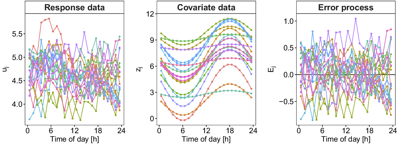
Figure 3. Sample of 20 generated output profiles (left), covariate profiles (middle), and error profiles (right).
3.2. Model training simulation results
Next, we perform the model training pipeline of the CAFDA-SHM framework (steps 0–3, the “orange part” in Figure 2). We repeated the procedure of generating data (according to Section 3.1) and model training 100 times to gain insights into the model performance and possible parameter estimation variability. Figure 4 illustrates the results comparing the true functions $ \tilde{\alpha}(t) $
,
$ \tilde{\alpha}(t) $
, $ {\alpha}_0+f(z) $
, and
$ {\alpha}_0+f(z) $
, and $ {\phi}_r(t) $
,
$ {\phi}_r(t) $
, $ r=1,\dots, 3 $
, drawn in blue, to the estimates
$ r=1,\dots, 3 $
, drawn in blue, to the estimates $ \hat{\tilde{\alpha}}(t) $
,
$ \hat{\tilde{\alpha}}(t) $
, $ {\hat{\alpha}}_0+\hat{f}(z) $
,
$ {\hat{\alpha}}_0+\hat{f}(z) $
, $ {\hat{\phi}}_r(t) $
from the 100 simulation runs (gray), where each run consisted of a training set of
$ {\hat{\phi}}_r(t) $
from the 100 simulation runs (gray), where each run consisted of a training set of $ J=300 $ $ u $
- and
$ u $
- and $ z $
-profiles. The respective mean functions of the estimates are shown in red. The top-left figure shows the results for the centered functional intercept
$ z $
-profiles. The respective mean functions of the estimates are shown in red. The top-left figure shows the results for the centered functional intercept $ \tilde{\alpha}(t) $
and the top-right figure for the covariate effect plus the overall intercept
$ \tilde{\alpha}(t) $
and the top-right figure for the covariate effect plus the overall intercept $ {\alpha}_0+f(z) $
. The three figures in the bottom row show the results for eigenfunctions
$ {\alpha}_0+f(z) $
. The three figures in the bottom row show the results for eigenfunctions $ {\phi}_r(t) $
,
$ {\phi}_r(t) $
, $ r=\mathrm{1,2,3} $
. The red and blue curves are close, meaning that the trained models and their estimated functional components can approximate the true underlying functions well on average. In other words, the estimates are (nearly) unbiased. Also, the variation is relatively small, see the gray curves.
$ r=\mathrm{1,2,3} $
. The red and blue curves are close, meaning that the trained models and their estimated functional components can approximate the true underlying functions well on average. In other words, the estimates are (nearly) unbiased. Also, the variation is relatively small, see the gray curves.
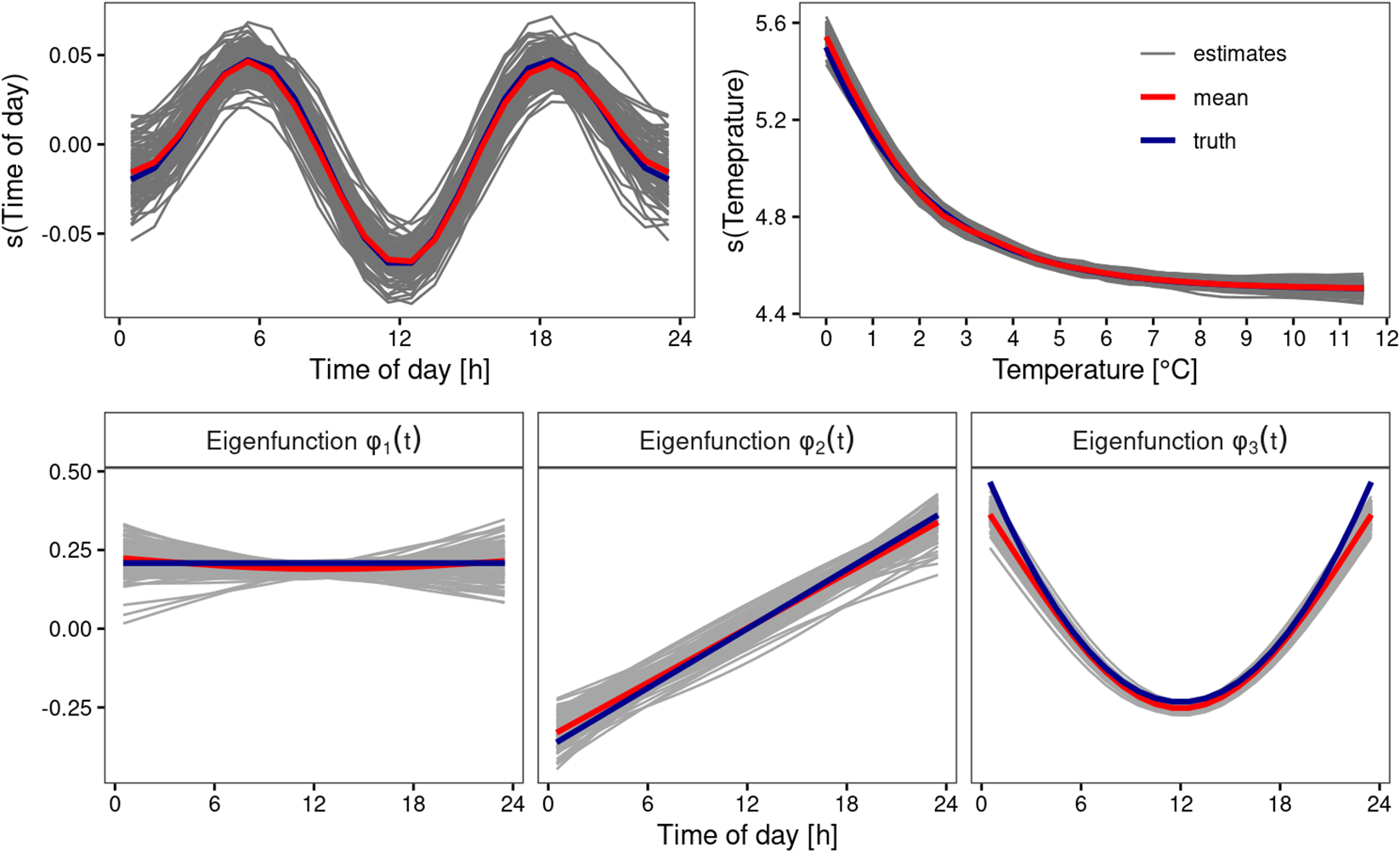
Figure 4. The estimates of the functional intercept (top-left) and the nonlinear covariate effect (top-right), as well as the estimated eigenfunctions of the structural component of the error process (bottom row). Shown in gray are the results for each of the 100 simulation runs, while the blue curves give the true functions, and the red curves the mean across the 100 runs.
3.3. Monitoring simulation results
In this section, the monitoring scheme (green part in Figure 2) is evaluated concerning the ARL performance in a Monte Carlo simulation. Specifically, for each of the 100 models from Section 3.2, the out-of-sample ARL is calculated by taking the average of the observed run lengths $ N $
over 10,000 replicates of the procedure with steps 1–7 given below. The control limit
$ N $
over 10,000 replicates of the procedure with steps 1–7 given below. The control limit $ {h}_4 $
is determined based on a prespecified ARL
$ {h}_4 $
is determined based on a prespecified ARL $ {}_0=100 $
(days), and the ARL is computed by the following procedure for Phase-II days
$ {}_0=100 $
(days), and the ARL is computed by the following procedure for Phase-II days $ g=1,2,\dots $
:
$ g=1,2,\dots $
:
-
1. Generate new covariate data
$ {z}_g(t) $
according to Section 3.1 (which produces the data in step 4.1 of Figure 2). -
2. Add a shift
$ \delta $
in one of the three components of
$ {\boldsymbol{\mu}}_0 $
to create
$ {\boldsymbol{\mu}}_1 $
and draw scores from the corresponding normal distribution to simulate the functional random effect
$ {w}_g(t) $
. -
3. Generate the output data
$ {u}_g\left({t}_i\right) $
at measurement points
$ {t}_1,\dots, {t}_{24} $
by adding the functional intercept, the fixed effect of temperature
$ f\left({z}_g\left({t}_i\right)\right) $
, the functional random effect
$ {w}_g\left({t}_i\right) $
, and white noise error
$ {\unicode{x025B}}_g\left({t}_i\right) $
, analogously to Section 3.1. This produces the data in step 4.2 of Figure 2. -
4. Predict the system output using the model from Phase I (compare Section 3.2) and compute the resulting
$ {\hat{E}}_g\left({t}_i\right) $
by subtracting the predicted from the observed system output. -
5. Calculate the scores
$ {\hat{\xi}}_{r,g} $
according to Eq. (10). -
6. Compute MEWMA and
$ {T}^2 $
statistic according to Eqs. (11) and (12). -
7. If
$ {T}^2>{h}_4 $
, note the run-length
$ N $
, else repeat steps 1–6 for the next profile (day).


The upper panel of Figure 5 shows ARL profiles on a logarithmic scale for shifts in the scores’ mean on a fine grid for $ \delta \in \left[0,3\right] $
with three different smoothing parameters
$ \delta \in \left[0,3\right] $
with three different smoothing parameters $ \lambda \in \{0.1,0.3,1\} $
. For a fair comparison, all three charts are calibrated to the same
$ \lambda \in \{0.1,0.3,1\} $
. For a fair comparison, all three charts are calibrated to the same $ {\mathrm{ARL}}_0=100 $
. However, note that the ARL of all three charts is slightly above 100 for the in-control scenario. This can be explained by the fact that the prediction (10) of the scores in the mixed model framework imposes a Ridge-type penalty and, hence, a form of shrinkage toward zero. Furthermore, it can be seen that the choice of the smoothing parameter
$ {\mathrm{ARL}}_0=100 $
. However, note that the ARL of all three charts is slightly above 100 for the in-control scenario. This can be explained by the fact that the prediction (10) of the scores in the mixed model framework imposes a Ridge-type penalty and, hence, a form of shrinkage toward zero. Furthermore, it can be seen that the choice of the smoothing parameter $ \lambda $
influences the ARL
$ \lambda $
influences the ARL $ {}_1 $
profiles and, thus, the detection speed of the out-of-control scenario. As mentioned in Section 2.3, small values of
$ {}_1 $
profiles and, thus, the detection speed of the out-of-control scenario. As mentioned in Section 2.3, small values of $ \lambda $
lead to quicker detection of small changes, while charts using, e.g.,
$ \lambda $
lead to quicker detection of small changes, while charts using, e.g., $ \lambda =1 $
(the pink curves in Figure 5) have a shorter run length on average for substantial shifts. Comparing, for example, the crossing points of the ARL profiles for different shift sizes
$ \lambda =1 $
(the pink curves in Figure 5) have a shorter run length on average for substantial shifts. Comparing, for example, the crossing points of the ARL profiles for different shift sizes $ \delta $
for the three components in the upper row, one could conclude that a shift in the third score would be detected more quickly than in the first component. However, this effect is blurred as the variances
$ \delta $
for the three components in the upper row, one could conclude that a shift in the third score would be detected more quickly than in the first component. However, this effect is blurred as the variances $ {\nu}_r $
of the principal components decrease for larger
$ {\nu}_r $
of the principal components decrease for larger $ r $
, see Section 3.1. Hence, a version with standardized shift size
$ r $
, see Section 3.1. Hence, a version with standardized shift size $ \frac{\delta }{\nu_r} $
is plotted in Figure 5 (bottom row) to give a clearer picture of the detection speed in regards to each component. It shows that the detection speed is comparable for all three components.
$ \frac{\delta }{\nu_r} $
is plotted in Figure 5 (bottom row) to give a clearer picture of the detection speed in regards to each component. It shows that the detection speed is comparable for all three components.
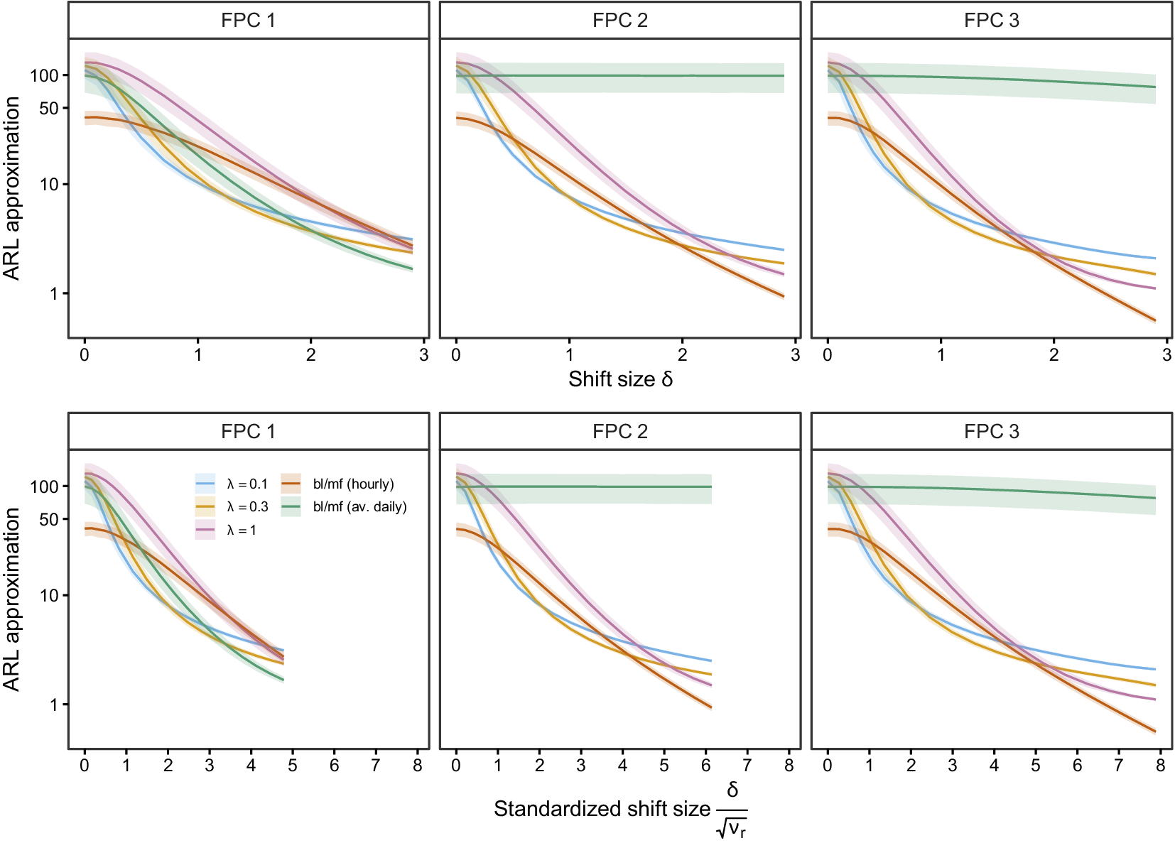
Figure 5. ARL profiles (averaged over the 100 models/training datasets from Section 3.2) on a logarithmic scale for a shift in the scores’ mean. Considered are MEWMA control charts as proposed in Section 2.3 with different smoothing parameter $ \lambda $
(blue, orange, pink) and Shewhart charts based on hourly (brown) or 24 h averaged (green) misfits of a piecewise linear model, displayed for absolute shift size
$ \lambda $
(blue, orange, pink) and Shewhart charts based on hourly (brown) or 24 h averaged (green) misfits of a piecewise linear model, displayed for absolute shift size $ \delta $
(top row) and standardized shift size
$ \delta $
(top row) and standardized shift size $ \frac{\delta }{\sqrt{\nu_r}} $
(bottom row). The shaded regions give the uncertainty concerning the ARL approximation in terms of
$ \frac{\delta }{\sqrt{\nu_r}} $
(bottom row). The shaded regions give the uncertainty concerning the ARL approximation in terms of $ \pm $
one standard deviation across the 100 models/training datasets from Section 3.2.
$ \pm $
one standard deviation across the 100 models/training datasets from Section 3.2.
For comparison, we show the results for two competing/existing approaches popular in SHM in brown and green in Figure 5. Specifically, the effect of temperature (compare the top-right panel of Figure 4) is captured through a so-called “bilinear” model, i.e., a piecewise linear model with one breakpoint. Then, the so-called “misfits” are calculated by subtracting the predicted values (hourly) from the measured eigenfrequencies. Finally, the (squared) normalized misfits can be used for monitoring, with control limits typically obtained as quantiles of a $ {\chi}^2 $
distribution. This approach is also called “Shewhart control chart” (see, e.g., Montgomery, Reference Montgomery2009). Following Maes et al. (Reference Maes, Van Meerbeeck, Reynders and Lombaert2022), we consider two versions: (i) hourly data are monitored directly (the brown lines in Figure 5), and (ii) hourly misfits are averaged over 24 h (i.e., days) before calculating the normalized misfits (the green lines in Figure 5). It is seen that averaging misfits over 24 h works very well for detecting shifts in the first (functional) principal component. The reason is that the averaged misfit approximates the first score well, i.e., it is nearly proportional to the first score; compare equation (9) and the first eigenfunction in Figure 4 (bottom-left), which is constant over the day. However, if the shift occurs in the second or third component, the averaged misfits cannot detect this (compare the results/green lines for FPC1 and FPC2/FPC3 in Figure 5). This is because the eigenfunctions are orthogonal (see the bottom row of Figure 4). The approach (i), which monitors the hourly misfits, on the other hand, can detect shifts in all three components.Footnote 1 However, it is severely miscalibrated, as the average time-to-signal on the in-control data (i.e., for a shift size
$ {\chi}^2 $
distribution. This approach is also called “Shewhart control chart” (see, e.g., Montgomery, Reference Montgomery2009). Following Maes et al. (Reference Maes, Van Meerbeeck, Reynders and Lombaert2022), we consider two versions: (i) hourly data are monitored directly (the brown lines in Figure 5), and (ii) hourly misfits are averaged over 24 h (i.e., days) before calculating the normalized misfits (the green lines in Figure 5). It is seen that averaging misfits over 24 h works very well for detecting shifts in the first (functional) principal component. The reason is that the averaged misfit approximates the first score well, i.e., it is nearly proportional to the first score; compare equation (9) and the first eigenfunction in Figure 4 (bottom-left), which is constant over the day. However, if the shift occurs in the second or third component, the averaged misfits cannot detect this (compare the results/green lines for FPC1 and FPC2/FPC3 in Figure 5). This is because the eigenfunctions are orthogonal (see the bottom row of Figure 4). The approach (i), which monitors the hourly misfits, on the other hand, can detect shifts in all three components.Footnote 1 However, it is severely miscalibrated, as the average time-to-signal on the in-control data (i.e., for a shift size $ \delta =0 $
) is below 50 days (instead of 100). The reason is that the common assumption of uncorrelated misfits was used to determine the control limits. The hourly misfits, however, are strongly correlated. Of course, one could try to account for this using some parametric model, such as first-order autocorrelation, when calculating the control limits. In practice, however, it is typically unclear which (parametric) model to use. As pointed out, one advantage of the FPCA-based approach is that the correlation structure is estimated semiparametrically from the data. So, generally speaking, it can be concluded that the proposed FDA-based approach can extract much more information from the data in a statistically sound way than simpler approaches considering misfits.
$ \delta =0 $
) is below 50 days (instead of 100). The reason is that the common assumption of uncorrelated misfits was used to determine the control limits. The hourly misfits, however, are strongly correlated. Of course, one could try to account for this using some parametric model, such as first-order autocorrelation, when calculating the control limits. In practice, however, it is typically unclear which (parametric) model to use. As pointed out, one advantage of the FPCA-based approach is that the correlation structure is estimated semiparametrically from the data. So, generally speaking, it can be concluded that the proposed FDA-based approach can extract much more information from the data in a statistically sound way than simpler approaches considering misfits.
4. Applications to structural health monitoring data
In what follows, we will apply our CAFDA-SHM framework to the data from the KW51 bridge in a first case study in Section 4.1. We focus on the system’s dynamic response in terms of natural frequencies. Section 4.2 provides a second case study considering displacement measurements from a reinforced concrete motorway bridge, the so-called “Sachsengraben viaduct.”
4.1. The KW 51 railway bridge
KW51 is a steel railway bridge of the bowstring type, with two curved, ballasted, electrified tracks. It is 115 m long, 12.4 m wide, and located between Leuven and Brussels, Belgium, on the railway line L36N. The bridge was monitored from October 2, 2018 to January 15, 2020, with a retrofitting period from May 15 to September 27, 2019. Various quantities, such as the steel surface temperature or relative humidity, were measured on an hourly basis (Maes and Lombaert, Reference Maes and Lombaert2020; Maes et al., Reference Maes, Van Meerbeeck, Reynders and Lombaert2022). Due to the large amounts of data, only fragments of the raw acceleration and inclination data are available for reuse/download. Maes and Lombaert (Reference Maes and Lombaert2020) employed operational modal analysis (OMA) to determine the modal parameters with the reference-based covariance-driven stochastic subspace (SSI-cov/ref) algorithm on an hourly basis as well. The natural frequencies of 14 modes are available for the entire monitoring period and are described in detail in Maes and Lombaert (Reference Maes and Lombaert2021). Here, we will focus on the data for mode 6, with parts of it already shown in Figure 1. In addition, we will consider two potentially confounding variables, temperature at the bridge deck level and relative humidity, both measured directly at the bridge. In a preprocessing step, some extreme outliers were removed from the dataset. Those outliers correspond to some data points that resulted from abnormal bridge behavior on particularly cold days (Maes and Lombaert, Reference Maes and Lombaert2021; Maes et al., Reference Maes, Van Meerbeeck, Reynders and Lombaert2022). Eventually, 225 daily profiles were available for modeling before the retrofitting started. In Sections 4.1.1–4.1.2 below, we will discuss the CAFDA results for different model specifications, including the basic model with one covariate “temperature” only and two versions of an extended model with both temperature and relative humidity included as covariates. All those models allow for nonlinear covariate effects, whereas earlier analyses of the KW51 data (Anastasopoulos et al., Reference Anastasopoulos, De Roeck and Reynders2021; Maes et al., Reference Maes, Van Meerbeeck, Reynders and Lombaert2022) focused on linear modeling. Finally, some results for monitoring Phase-II data will be shown in Section 4.1.3. To prevent the end of the in-control phase from coinciding with the start of the retrofitting, Phase I is limited to 200 observed profiles (between October 2, 2018, and April 19, 2019) for the model training. Out of those 200 profiles of natural frequencies, 129 profiles are observed over 24 h of the day, while the rest have between 4% and 100% of missing values. Concerning the temperature and humidity curves, 57 and 66 profiles have 4%–100% missing values, respectively. Overall, the percentage of missing values is high, at 63%.
4.1.1. Results for the basic model
We start with the basic model and the parametrization in (8). It includes an overall intercept $ {\alpha}_0 $
, a functional intercept
$ {\alpha}_0 $
, a functional intercept $ \tilde{\alpha}(t) $
, a potentially nonlinear temperature effect
$ \tilde{\alpha}(t) $
, a potentially nonlinear temperature effect $ f(z) $
, and the structural component
$ f(z) $
, and the structural component $ {w}_j(t) $
of the error process. After estimating the fixed effects of the initial model in step 1 of Figure 2, we apply the FPCA on
$ {w}_j(t) $
of the error process. After estimating the fixed effects of the initial model in step 1 of Figure 2, we apply the FPCA on $ 148 $
residual profiles (those with sufficient data points of both the natural frequencies and temperature curves available) to extract the eigenfunctions of the functional random effects as described in Section 2.2.2. The number of components to extract is chosen such that 99% of the variance with respect to the smoothed covariance matrix is explained. In step 3 of our modeling framework, we refit the basic model, incorporating the eigenfunctions to account for the functional random effects.
$ 148 $
residual profiles (those with sufficient data points of both the natural frequencies and temperature curves available) to extract the eigenfunctions of the functional random effects as described in Section 2.2.2. The number of components to extract is chosen such that 99% of the variance with respect to the smoothed covariance matrix is explained. In step 3 of our modeling framework, we refit the basic model, incorporating the eigenfunctions to account for the functional random effects.
Figure 6 shows the estimates $ {\hat{\phi}}_1(t),\dots, {\hat{\phi}}_4(t) $
of the eigenfunctions. Note that the first two eigenfunctions already explain about 85.6% of the variance of the structural part
$ {\hat{\phi}}_1(t),\dots, {\hat{\phi}}_4(t) $
of the eigenfunctions. Note that the first two eigenfunctions already explain about 85.6% of the variance of the structural part $ {w}_j(t) $
of the error process. The first three eigenfunctions have straightforward and physically interpretable shapes. The first eigenfunction has almost the shape of a horizontal line, which means that the first principal component represents the overall extent of the daily error in terms of a weighted average with maximum weights in the early afternoon. The second component describes the difference in the errors between the morning and evening hours, whereas the third component corresponds to the contrast between night and day. The last component, component 4, is less clear, but this component accounts for less than 5.6% of the variance of
$ {w}_j(t) $
of the error process. The first three eigenfunctions have straightforward and physically interpretable shapes. The first eigenfunction has almost the shape of a horizontal line, which means that the first principal component represents the overall extent of the daily error in terms of a weighted average with maximum weights in the early afternoon. The second component describes the difference in the errors between the morning and evening hours, whereas the third component corresponds to the contrast between night and day. The last component, component 4, is less clear, but this component accounts for less than 5.6% of the variance of $ {w}_j(t) $
.
$ {w}_j(t) $
.
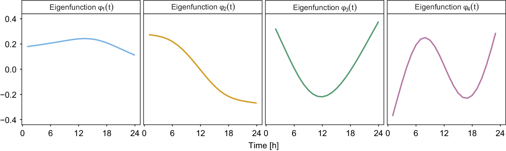
Figure 6. Estimates of the eigenfunctions of the functional random effects in the basic model for the KW51 data.
Figure 7 shows the centered functional intercept $ \tilde{\alpha} $
and the nonlinear fixed effect
$ \tilde{\alpha} $
and the nonlinear fixed effect $ f(z) $
of temperature
$ f(z) $
of temperature $ z $
on the natural frequency of mode 6, which is also centered across the data observed. The functional intercept can be interpreted as a recurring daily pattern. The gray-shaded areas represent the estimated effects’ uncertainty in terms of pointwise 95% confidence intervals. Comparing both effects, we find that the effect of the functional intercept is flat over the day, which means that a recurring daily pattern, if any, is very weak if the steel temperature is taken into account. In contrast, the temperature effect shows a pronounced nonlinear shape with a kink between 2°C and 3°C. This confirms statements in the literature that the influence of temperature on the dynamic response is stronger at lower temperatures (Xia et al., Reference Xia, Chen, Weng, Ni and Xu2012; Han et al., Reference Han, Ma, Xu and Liu2021). Figure 7 (right) also shows another benefit of the nonlinear approach compared to classical linear regression by Maes et al. (Reference Maes, Van Meerbeeck, Reynders and Lombaert2022), who simply omitted the data below 2°C. Our method can also utilize the data from the colder days and thus capture the nonlinear temperature effect well.
$ z $
on the natural frequency of mode 6, which is also centered across the data observed. The functional intercept can be interpreted as a recurring daily pattern. The gray-shaded areas represent the estimated effects’ uncertainty in terms of pointwise 95% confidence intervals. Comparing both effects, we find that the effect of the functional intercept is flat over the day, which means that a recurring daily pattern, if any, is very weak if the steel temperature is taken into account. In contrast, the temperature effect shows a pronounced nonlinear shape with a kink between 2°C and 3°C. This confirms statements in the literature that the influence of temperature on the dynamic response is stronger at lower temperatures (Xia et al., Reference Xia, Chen, Weng, Ni and Xu2012; Han et al., Reference Han, Ma, Xu and Liu2021). Figure 7 (right) also shows another benefit of the nonlinear approach compared to classical linear regression by Maes et al. (Reference Maes, Van Meerbeeck, Reynders and Lombaert2022), who simply omitted the data below 2°C. Our method can also utilize the data from the colder days and thus capture the nonlinear temperature effect well.
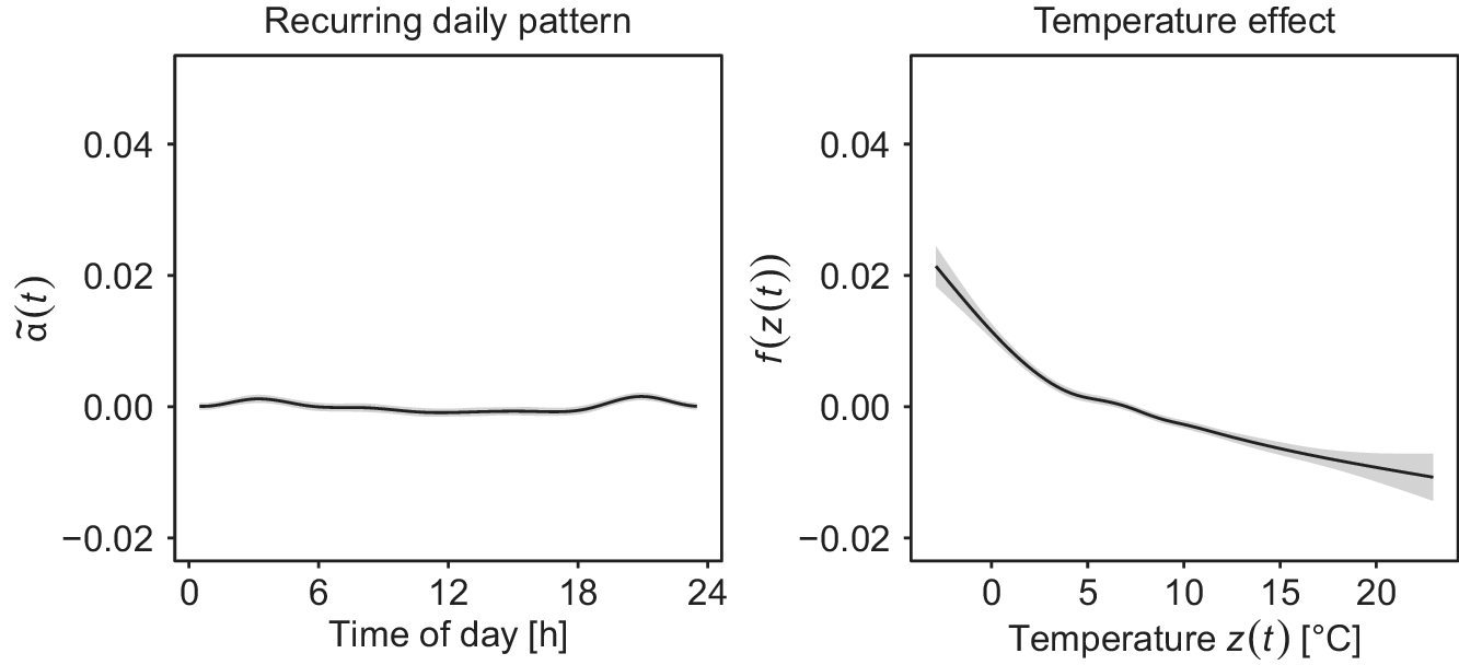
Figure 7. Results of the basic functional modeling approach (1) for the functional intercept (left) and the nonlinear effect of temperature (right) on the natural frequency (mode 6) of the KW51 bridge.
4.1.2. Results for extended models
Next, we extend the basic model by including relative humidity as a second covariate in an additive way. We now have $ {u}_j(t)={\alpha}_0+\tilde{\alpha}\left(t,{d}_j\right)+{f}_1\left({z}_1(t)\right)+{f}_2\left({z}_2(t)\right)+{E}_j(t) $
,
$ {u}_j(t)={\alpha}_0+\tilde{\alpha}\left(t,{d}_j\right)+{f}_1\left({z}_1(t)\right)+{f}_2\left({z}_2(t)\right)+{E}_j(t) $
, $ j=1,\dots, J $
,
$ j=1,\dots, J $
, $ t\in \mathcal{T} $
, where
$ t\in \mathcal{T} $
, where $ {f}_1 $
and
$ {f}_1 $
and $ {f}_2 $
denote the potentially nonlinear effects of temperature and relative humidity, respectively. Due to the limited number of datasets where the two covariates are measured jointly, the number of daily profiles that can be used for parameter estimation reduces to
$ {f}_2 $
denote the potentially nonlinear effects of temperature and relative humidity, respectively. Due to the limited number of datasets where the two covariates are measured jointly, the number of daily profiles that can be used for parameter estimation reduces to $ J=100 $
days. As before, we proceed with the model training steps 1–3 from Figure 2. Figure 8 shows the results for the final model, the (centered) two-dimensional functional intercept (left), and the effects of temperature (middle) and relative humidity (right). The flat intercept indicates that there are no daily and yearly patterns, such as seasonal effects, that cannot be explained through the covariates in the model. The (explicit) temperature effect
$ J=100 $
days. As before, we proceed with the model training steps 1–3 from Figure 2. Figure 8 shows the results for the final model, the (centered) two-dimensional functional intercept (left), and the effects of temperature (middle) and relative humidity (right). The flat intercept indicates that there are no daily and yearly patterns, such as seasonal effects, that cannot be explained through the covariates in the model. The (explicit) temperature effect $ {f}_1 $
shows a similar nonlinear behavior as seen with the basic model in Figure 7. The effect
$ {f}_1 $
shows a similar nonlinear behavior as seen with the basic model in Figure 7. The effect $ {f}_2 $
for relative humidity is much smaller but still present, as can also be seen from the increased
$ {f}_2 $
for relative humidity is much smaller but still present, as can also be seen from the increased $ {R}^2 $
of
$ {R}^2 $
of $ 0.52 $
, compared to
$ 0.52 $
, compared to $ 0.43 $
for the basic model with temperature as the only covariate, see Table 1.
$ 0.43 $
for the basic model with temperature as the only covariate, see Table 1.
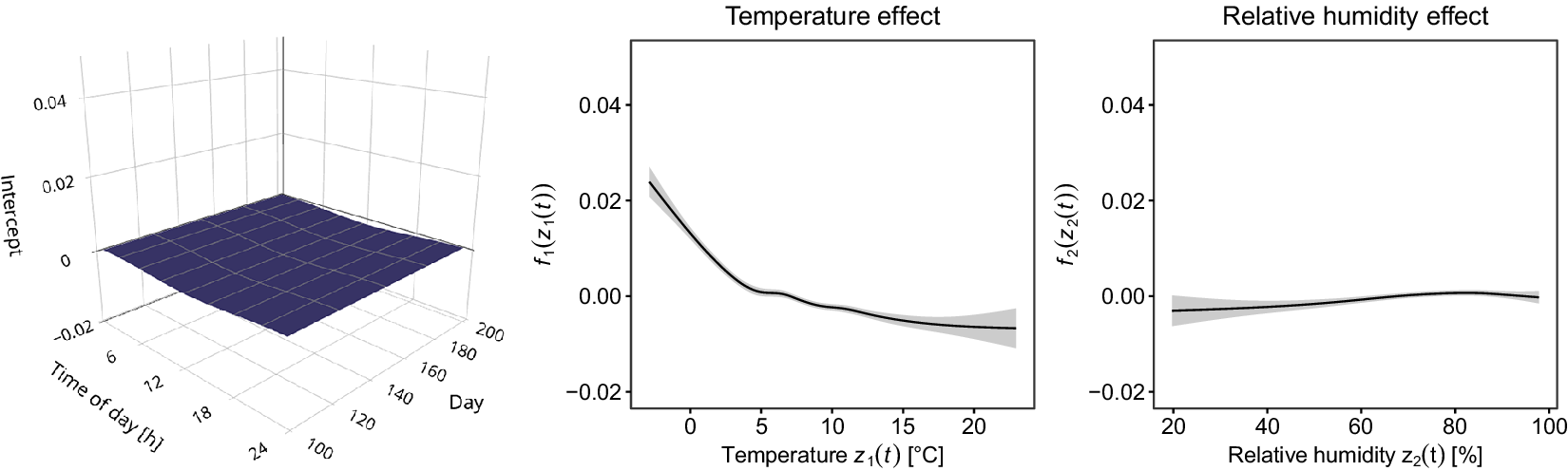
Figure 8. Results of the extended functional modeling approach showing a two-dimensional functional intercept (left) and the additive, potentially nonlinear effects of temperature (middle) and relative humidity (right) on the natural frequency (mode 6) of the KW51 bridge.
Table 1. Summary of the $ {R}^2 $
, overall number of observations, and number of profiles used in Phase I for the different compared models
$ {R}^2 $
, overall number of observations, and number of profiles used in Phase I for the different compared models

As a second extension, we replace the additive effects from above by the term $ {f}_{12}\Big({z}_{j1}(t), $ $ {z}_{j2}(t)\Big) $
for the two covariates, allowing for an interacting effect on the system outputs. Figure 9 shows the resulting (centered) two-dimensional functional intercept
$ {z}_{j2}(t)\Big) $
for the two covariates, allowing for an interacting effect on the system outputs. Figure 9 shows the resulting (centered) two-dimensional functional intercept $ \tilde{\alpha}\left(t,{d}_j\right) $
and the surface
$ \tilde{\alpha}\left(t,{d}_j\right) $
and the surface $ {f}_{12} $
taking interactions of temperature and relative humidity into account in a smooth, nonparametric way. As we can see, the strongest effect is along the temperature axis, but humidity is also relevant, with its most substantial effect around 10°C. As before, the functional intercept is flat, indicating no further daily or seasonal patterns. The reason why the yellow color of the surface in the right plot of Figure 9 is only seen for low humidity is that no data points with negative temperatures and high humidity are available. That is why
$ {f}_{12} $
taking interactions of temperature and relative humidity into account in a smooth, nonparametric way. As we can see, the strongest effect is along the temperature axis, but humidity is also relevant, with its most substantial effect around 10°C. As before, the functional intercept is flat, indicating no further daily or seasonal patterns. The reason why the yellow color of the surface in the right plot of Figure 9 is only seen for low humidity is that no data points with negative temperatures and high humidity are available. That is why $ {f}_{12} $
cannot be fitted in that area, whereas data points with negative temperature and low humidity are found in the dataset. For the latter, the highest natural frequency values (of mode 6) are predicted as indicated by the yellow color. The overall model fit (
$ {f}_{12} $
cannot be fitted in that area, whereas data points with negative temperature and low humidity are found in the dataset. For the latter, the highest natural frequency values (of mode 6) are predicted as indicated by the yellow color. The overall model fit ( $ {R}^2=0.54 $
) is slightly better than with the additive model (compare Table 1) and, as such, considerably better than the basic model. In summary (see also Table 1), the temperature appears to be the most influential covariate. For comparison, using the two-dimensional intercept only in terms of an output-only approach leads to an
$ {R}^2=0.54 $
) is slightly better than with the additive model (compare Table 1) and, as such, considerably better than the basic model. In summary (see also Table 1), the temperature appears to be the most influential covariate. For comparison, using the two-dimensional intercept only in terms of an output-only approach leads to an $ {R}^2=0.25 $
, which is substantially lower than the
$ {R}^2=0.25 $
, which is substantially lower than the $ {R}^2=0.43 $
obtained with the basic model. Further note: If the monitoring as proposed here (the green part of Figure 2) is to use the results of the output-only model, training data over an entire year must be available because otherwise, for some future Phase-II days, no predictions and, thus, no error profiles for calculating the scores are available. In general, this is also true for other models like Figures 8 and 9 with two-dimensional intercepts, but in the specific case of KW51 considered here, those intercepts are flat, meaning that they are irrelevant for prediction. Consequently, those models can be used for monitoring, as illustrated in Section 4.1.3 below. Monitoring with an output-only model will be considered in Section 4.2.
$ {R}^2=0.43 $
obtained with the basic model. Further note: If the monitoring as proposed here (the green part of Figure 2) is to use the results of the output-only model, training data over an entire year must be available because otherwise, for some future Phase-II days, no predictions and, thus, no error profiles for calculating the scores are available. In general, this is also true for other models like Figures 8 and 9 with two-dimensional intercepts, but in the specific case of KW51 considered here, those intercepts are flat, meaning that they are irrelevant for prediction. Consequently, those models can be used for monitoring, as illustrated in Section 4.1.3 below. Monitoring with an output-only model will be considered in Section 4.2.
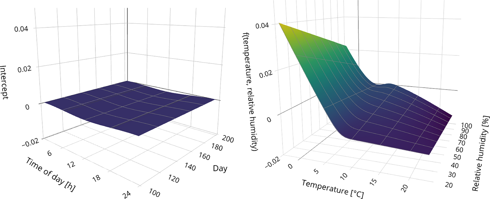
Figure 9. Results of the extended functional modeling approach showing a two-dimensional functional intercept $ \alpha \left(t,{d}_j\right) $
(left) and a two-dimensional functional interaction of temperature and relative humidity
$ \alpha \left(t,{d}_j\right) $
(left) and a two-dimensional functional interaction of temperature and relative humidity $ {f}_{12}\left({z}_{j1}(t),{z}_{j2}(t)\right) $
(right) on the natural frequency (mode 6) of the KW51 bridge.
$ {f}_{12}\left({z}_{j1}(t),{z}_{j2}(t)\right) $
(right) on the natural frequency (mode 6) of the KW51 bridge.
4.1.3. Anomaly detection
Finally, we apply the second part of the CAFDA-SHM framework, the monitoring scheme, to the natural frequency data (mode 6) of the KW51 bridge, including the retrofitting data for online monitoring as in Maes et al. (Reference Maes, Van Meerbeeck, Reynders and Lombaert2022). Two MEWMA chart configurations with different $ \lambda $
are chosen, and two functional models are compared: the basic model (Section 4.1.1) and the best-performing model according to Table 1, the extended model with interaction term. As mentioned, Phase I consists of the first 200 days. However, only 3411 and 2268 observations, or 148 and 100 profiles, could be used for the basic and the extended model, respectively, due to data availability, compare Table 1. The control charts are calibrated to an ARL
$ \lambda $
are chosen, and two functional models are compared: the basic model (Section 4.1.1) and the best-performing model according to Table 1, the extended model with interaction term. As mentioned, Phase I consists of the first 200 days. However, only 3411 and 2268 observations, or 148 and 100 profiles, could be used for the basic and the extended model, respectively, due to data availability, compare Table 1. The control charts are calibrated to an ARL $ {}_0=370.4 $
applying thresholds
$ {}_0=370.4 $
applying thresholds $ {h}_4=16.25 $
and
$ {h}_4=16.25 $
and $ {h}_4=15.83 $
for
$ {h}_4=15.83 $
for $ \lambda =1 $
and
$ \lambda =1 $
and $ \lambda =0.3 $
, respectively. Utilizing the estimated parameters of the basic model and the extended model, respectively, and the incoming data, the scores
$ \lambda =0.3 $
, respectively. Utilizing the estimated parameters of the basic model and the extended model, respectively, and the incoming data, the scores $ {\hat{\xi}}_{r,g} $
from (10),
$ {\hat{\xi}}_{r,g} $
from (10), $ m=4 $
, are used in (12) to calculate the control statistic
$ m=4 $
, are used in (12) to calculate the control statistic $ {T}_g^2 $
for day
$ {T}_g^2 $
for day $ g $
(compare Section 2.3).
$ g $
(compare Section 2.3).
Figure 10 displays the resulting control charts. In all MEWMA charts, online monitoring begins in Phase II after the dashed line, with the retrofitting period marked through the gray shaded area. If using the basic model and the control chart with $ \lambda =1 $
(top-left), the first signal is seen on June 8, 2019, while the chart, which uses the extended model (top-right) issues the first signal 6 days earlier on June 2, 2019, thus showing a higher sensitivity. Thereafter, both charts indicate a clear shift in the natural frequency of mode 6. The control charts with
$ \lambda =1 $
(top-left), the first signal is seen on June 8, 2019, while the chart, which uses the extended model (top-right) issues the first signal 6 days earlier on June 2, 2019, thus showing a higher sensitivity. Thereafter, both charts indicate a clear shift in the natural frequency of mode 6. The control charts with $ \lambda =0.3 $
(bottom-row) show a false alarm on January 24–27, 2019, for the basic model, and on January 26 and 27, 2019 for the extended model, respectively. The bottom-row panels also reveal that compared to
$ \lambda =0.3 $
(bottom-row) show a false alarm on January 24–27, 2019, for the basic model, and on January 26 and 27, 2019 for the extended model, respectively. The bottom-row panels also reveal that compared to $ \lambda =1 $
, an alarm was triggered on May 26, 2019, so 11 days earlier in both charts. However, comparing the different scenarios, it is noticeable that all four control charts issue several signals in a row, indicating a sustained change in the process within the retrofitting (gray shaded area).
$ \lambda =1 $
, an alarm was triggered on May 26, 2019, so 11 days earlier in both charts. However, comparing the different scenarios, it is noticeable that all four control charts issue several signals in a row, indicating a sustained change in the process within the retrofitting (gray shaded area).
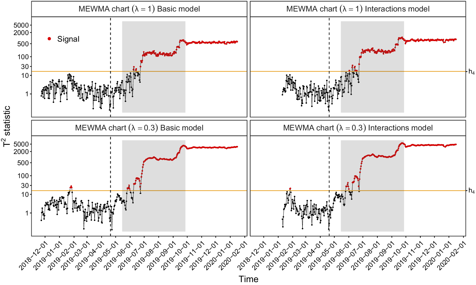
Figure 10. MEWMA control charts for $ \lambda =1 $
(top row) and
$ \lambda =1 $
(top row) and $ \lambda =0.3 $
(bottom row), on a logarithmic y-axis, using the basic (left column) and extended functional model with interactions (right column) for the KW51 bridge, including the retrofitting period (gray shaded area).
$ \lambda =0.3 $
(bottom row), on a logarithmic y-axis, using the basic (left column) and extended functional model with interactions (right column) for the KW51 bridge, including the retrofitting period (gray shaded area).
In summary, employing our CAFDA-SHM framework, the control charts detect a change in the bridge’s behavior caused by retrofitting, with faster detection being achieved through MEWMA parameterizations with $ \lambda <1 $
. Note, if using the misfits from the piecewise linear model, analogously to the simulation study in Section 3 and Maes et al. (Reference Maes, Van Meerbeeck, Reynders and Lombaert2022), not only the hourly (as in Section 3) but also the 24 h averaged misfits are highly correlated in time, leading to miscalibrated control limits. That is why we only showed the results for CAFDA-SHM here. Also note that we considered mode 6 for illustration and evaluation because the corresponding eigenfrequencies show the typical, nonlinear behavior reported in the literature (Han et al., Reference Han, Ma, Xu and Liu2021; Maes et al., Reference Maes, Van Meerbeeck, Reynders and Lombaert2022; Peeters and De Roeck, Reference Peeters and De Roeck2001). Similar behavior is found for modes 3, 9, and 13 of the KW51, and results obtained through CAFDA-SHM are also very similar.
$ \lambda <1 $
. Note, if using the misfits from the piecewise linear model, analogously to the simulation study in Section 3 and Maes et al. (Reference Maes, Van Meerbeeck, Reynders and Lombaert2022), not only the hourly (as in Section 3) but also the 24 h averaged misfits are highly correlated in time, leading to miscalibrated control limits. That is why we only showed the results for CAFDA-SHM here. Also note that we considered mode 6 for illustration and evaluation because the corresponding eigenfrequencies show the typical, nonlinear behavior reported in the literature (Han et al., Reference Han, Ma, Xu and Liu2021; Maes et al., Reference Maes, Van Meerbeeck, Reynders and Lombaert2022; Peeters and De Roeck, Reference Peeters and De Roeck2001). Similar behavior is found for modes 3, 9, and 13 of the KW51, and results obtained through CAFDA-SHM are also very similar.
4.2. The Sachsengraben viaduct
This section presents an application of the CAFDA-SHM framework on a second real-world SHM dataset, the OSIMABFootnote 2 dataset (Bundesanstalt für Straßenwesen (BASt), 2023), which contains measurements from the Sachsengraben bridge, see Figure 11. The bridge is located on the A45 motorway in Germany and was constructed in 1971. It spans 98 m and is made of prestressed concrete. The bridge’s cross-section consists of a single-cell box girder with a construction height of 2.8 m. The webs, floor, and deck slab also have coves; the end and support cross girders are stiffened. There are two separate substructures, and we will only focus on the northern one. The superstructure has three fields, divided by pillars. The two outer fields are 30 m long, while the middle field is 38 m long (Bundesanstalt für Straßenwesen (BASt), 2021).
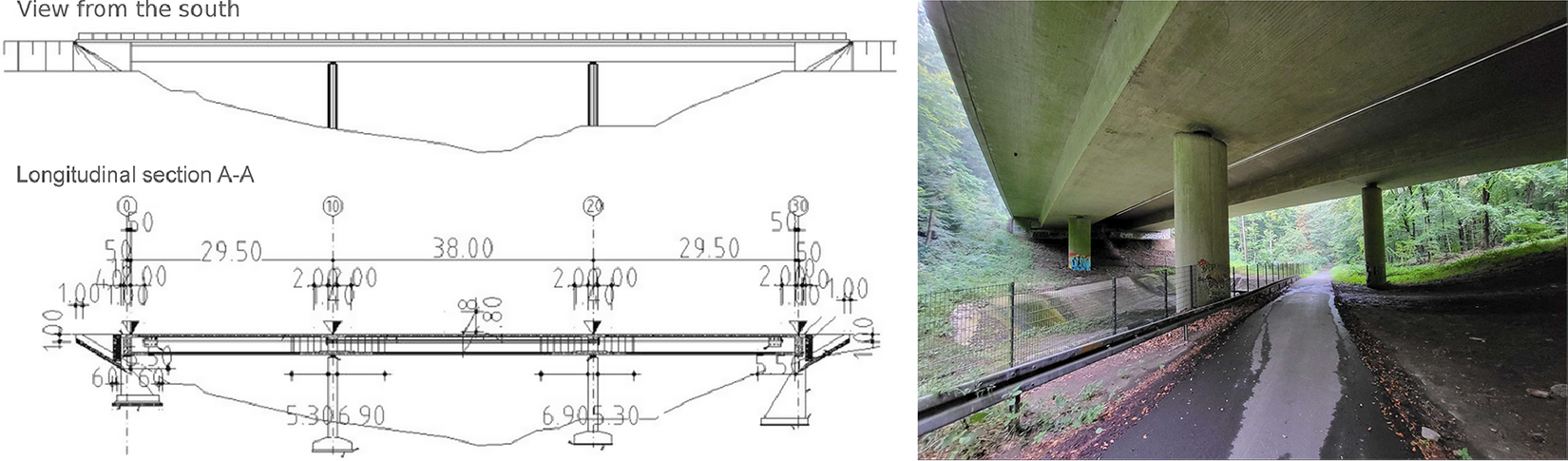
Figure 11. Schematic representation (left) of the Sachsengraben viaduct from the OSIMAB report (Bundesanstalt für Straßenwesen (BASt), 2021) and a photo of the bridge in 2023 (right).
Displacement was measured with eight displacement sensors per superstructure for 18 months, from January 1, 2020 to August 1, 2021 and with a sampling frequency of 100 Hz for the first 191 days and a 40-minute integration interval every hour. On day 191, the measurement switched to a 1 Hz sampling scheme, recording the data continuously. Ambient air temperature data recorded by a weather station and data from ten material temperature sensors with a sampling frequency of 1 Hz are also available. The entire dataset was collected in the OSIMAB project. A sample of the recorded measurement data is publicly available (Bundesanstalt für Straßenwesen (BASt), 2020), and the complete dataset is accessible via the Bundesanstalt für Straßenwesen (BASt) (2023).
Figure 12 shows the Phase-I profiles of one displacement sensor (N_F3_WA_NO, left) and measurements from the closest temperature sensor (N_F1_T_1, right) for 369 days. The dashed lines represent the first 191 days, from February 10, 2020 to August 19, 2020. The displacement and temperature measurements were resampled from the higher frequencies (100 and 1 Hz, respectively) by taking the median of the measurements within a 10-minute interval. This leads to a substantially larger number (144) of measurement points per day than with the KW51 bridge data, where the eigenfrequencies were obtained at 1-hour intervals. Furthermore, the 1.5-year measurement period means that data from each time of the year is available, and a two-dimensional intercept can be fitted that spans the entire year. The temperature values observed range from –10°C to 30°C. Out of 538 profiles in total, 287 displacement profiles and 461 temperature profiles did not exhibit any missing values, and overall, 20% of the data is missing.Footnote 3 This makes clear again that for SHM data, the methods used must be able to deal with missing data.
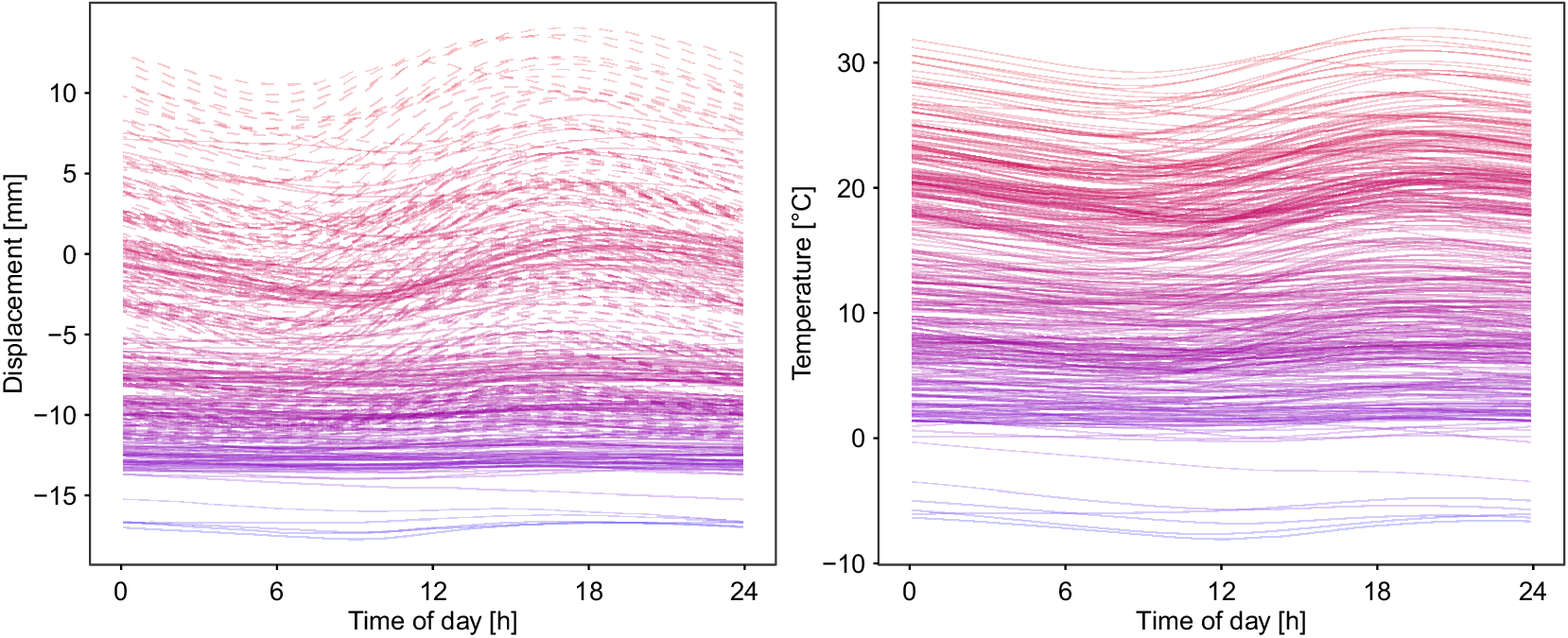
Figure 12. Phase-I profiles of displacement sensor N_F3_WA_NO (left) and temperature sensor N_F1_T_1 (right) with a 10-minute sampling rate. The profiles are highlighted in color according to their average daily temperature.
As mentioned above, the measurement recording process changed during Phase I. Nevertheless, we can still exploit the complete information available and capture a complete annual cycle in our framework. For doing so, we assume that changing the measurement systems’ sampling rate does not impact the external influence of the covariates — the fixed effects in our model $ {u}_j(t)={\alpha}_0+\tilde{\alpha}\left(t,{d}_j\right)+f\left({z}_j(t)\right)+{E}_j(t) $
,
$ {u}_j(t)={\alpha}_0+\tilde{\alpha}\left(t,{d}_j\right)+f\left({z}_j(t)\right)+{E}_j(t) $
, $ j=1,\dots, J $
,
$ j=1,\dots, J $
, $ t\in \mathcal{T} $
, where
$ t\in \mathcal{T} $
, where $ \tilde{\alpha} $
is the two-dimensional intercept (potentially) varying over both the course of the day and the year, and
$ \tilde{\alpha} $
is the two-dimensional intercept (potentially) varying over both the course of the day and the year, and $ f $
denotes the effect of the temperature. However, the functional random effects may show different behavior for the two time periods, which means that the eigenfunctions and variance components may differ. That is why two sets of residuals, before and after switching the sampling rate, were extracted to estimate two sets of eigenfunctions. It turned out that the eigenfunctions from the two time periods are very similar, but the variances differ substantially. Therefore, data were pooled to estimate a joint set of eigenfunctions, but variance components were allowed to differ between the two time periods when refitting the model in step 3 of Figure 2. Furthermore, as described in Sections 2.1 and 2.4, our model framework contains an output-only method as a special case in which only the system output of interest and its recorded timestamp are used, but no covariate data has to be recorded. In this case, the
$ f $
denotes the effect of the temperature. However, the functional random effects may show different behavior for the two time periods, which means that the eigenfunctions and variance components may differ. That is why two sets of residuals, before and after switching the sampling rate, were extracted to estimate two sets of eigenfunctions. It turned out that the eigenfunctions from the two time periods are very similar, but the variances differ substantially. Therefore, data were pooled to estimate a joint set of eigenfunctions, but variance components were allowed to differ between the two time periods when refitting the model in step 3 of Figure 2. Furthermore, as described in Sections 2.1 and 2.4, our model framework contains an output-only method as a special case in which only the system output of interest and its recorded timestamp are used, but no covariate data has to be recorded. In this case, the $ f\left({z}_j(t)\right) $
from the model above is omitted, and the only fixed effects left are the overall intercept
$ f\left({z}_j(t)\right) $
from the model above is omitted, and the only fixed effects left are the overall intercept $ {\alpha}_0 $
and the two-dimensional surface
$ {\alpha}_0 $
and the two-dimensional surface $ \tilde{\alpha}\left(t,{d}_j\right) $
, taking seasonal patterns into account. The latter function
$ \tilde{\alpha}\left(t,{d}_j\right) $
, taking seasonal patterns into account. The latter function $ \tilde{\alpha} $
is parameterized using a tensor product basis analogously to (13) with cyclic cubic regression splines in the
$ \tilde{\alpha} $
is parameterized using a tensor product basis analogously to (13) with cyclic cubic regression splines in the $ {d}_j $
-direction, which means that the function’s ends at the beginning and end of the year match up to the second derivative (Wood, Reference Wood2017). Using this reduced model, we could use all available Phase I data from the displacement sensor, without being limited by possibly missing covariate information.
$ {d}_j $
-direction, which means that the function’s ends at the beginning and end of the year match up to the second derivative (Wood, Reference Wood2017). Using this reduced model, we could use all available Phase I data from the displacement sensor, without being limited by possibly missing covariate information.
The left panel in Figure 13 visualizes $ \tilde{\alpha}\left(t,{d}_j\right) $
of the final output-only model with an
$ \tilde{\alpha}\left(t,{d}_j\right) $
of the final output-only model with an $ {R}^2=0.70 $
for the fixed effects. We can clearly see a yearly pattern with (on average) lower output values in the winter and higher values in the summer. The reason for these seasonal effects in the output-only model becomes clear from the middle and right panels of Figure 13, where the resulting estimates of the fixed effects in the extended model with the temperature included are shown. Now the two-dimensional intercept (middle) is rather flat over the year, indicating that the seasonal effects seen before were mainly caused by temperature variation. The explicit temperature effect on displacement in terms of the estimated
$ {R}^2=0.70 $
for the fixed effects. We can clearly see a yearly pattern with (on average) lower output values in the winter and higher values in the summer. The reason for these seasonal effects in the output-only model becomes clear from the middle and right panels of Figure 13, where the resulting estimates of the fixed effects in the extended model with the temperature included are shown. Now the two-dimensional intercept (middle) is rather flat over the year, indicating that the seasonal effects seen before were mainly caused by temperature variation. The explicit temperature effect on displacement in terms of the estimated $ f $
is shown in the right panel of Figure 13. This effect is almost linear with a tiny kink at around 15°C, which confirms similar results found in the literature, compare, e.g., Han et al. (Reference Han, Ma, Xu and Liu2021). In summary, it can be concluded that by specifying a two-dimensional functional intercept in the output-only model, we can already account for some of the environmental effects without the need to record corresponding covariate information. Consequently, if using an output-only approach to adjust for environmental influences, such a functional intercept should always be included if training data are available over a sufficiently long period.
$ f $
is shown in the right panel of Figure 13. This effect is almost linear with a tiny kink at around 15°C, which confirms similar results found in the literature, compare, e.g., Han et al. (Reference Han, Ma, Xu and Liu2021). In summary, it can be concluded that by specifying a two-dimensional functional intercept in the output-only model, we can already account for some of the environmental effects without the need to record corresponding covariate information. Consequently, if using an output-only approach to adjust for environmental influences, such a functional intercept should always be included if training data are available over a sufficiently long period.
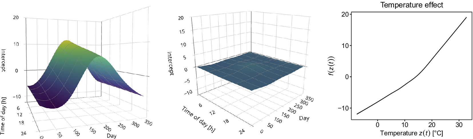
Figure 13. Results of the functional output-only model (left) and the extended functional modeling approach (middle) showing a two-dimensional functional intercept $ \overset{\sim }{\alpha }(t,{d}_j) $
and the (non)linear effect of temperature sensor N_F1_T_1 (right) on the displacement sensor N_F3_WA_NO.
$ \overset{\sim }{\alpha }(t,{d}_j) $
and the (non)linear effect of temperature sensor N_F1_T_1 (right) on the displacement sensor N_F3_WA_NO.
Similar to applying the control chart for anomaly detection in Section 4.1.3 and as shown in Figure 2, we set up the control charts, calibrating them to an ARL $ {}_0=370.4 $
. For monitoring purposes, only the second set of variance components is used, as those refer to the reconfigured measurement system with the new sampling rate. Figure 14 displays the control charts for
$ {}_0=370.4 $
. For monitoring purposes, only the second set of variance components is used, as those refer to the reconfigured measurement system with the new sampling rate. Figure 14 displays the control charts for $ \lambda =1 $
and a chart threshold
$ \lambda =1 $
and a chart threshold $ {h}_4=20.06 $
for the extended model and
$ {h}_4=20.06 $
for the extended model and $ {h}_4=11.83 $
for the output-only model. It is visible from both control charts that, besides the three false alarms in August and September 2021 in the Phase I data, the measurements before the dashed vertical line seem to be in control. The dashed line marks the beginning of the online monitoring on February 13, 2021. Bundesanstalt für Straßenwesen (BASt) (2021) reported that a sensor malfunction induced by a rust film blocking the sensor was noticed and confirmed at the end of March. The control chart utilizing the extended model in Figure 14 (left) detects this anomaly. However, it additionally detects some irregularities at the end of February. An explanation for this could be that the sensor malfunction already started before the end of March, and the control chart detected this. In contrast, the control chart using the output-only model (right) slightly fails to detect the anomaly. However, a modified control chart setup with
$ {h}_4=11.83 $
for the output-only model. It is visible from both control charts that, besides the three false alarms in August and September 2021 in the Phase I data, the measurements before the dashed vertical line seem to be in control. The dashed line marks the beginning of the online monitoring on February 13, 2021. Bundesanstalt für Straßenwesen (BASt) (2021) reported that a sensor malfunction induced by a rust film blocking the sensor was noticed and confirmed at the end of March. The control chart utilizing the extended model in Figure 14 (left) detects this anomaly. However, it additionally detects some irregularities at the end of February. An explanation for this could be that the sensor malfunction already started before the end of March, and the control chart detected this. In contrast, the control chart using the output-only model (right) slightly fails to detect the anomaly. However, a modified control chart setup with $ \lambda <1 $
(not shown here) would increase the chart’s detection sensitivity and lead to signals in Phase II. In summary, it can be stated that although the output-only model takes seasonal patterns caused by environmental effects into account, it is beneficial to account for these effects more explicitly.
$ \lambda <1 $
(not shown here) would increase the chart’s detection sensitivity and lead to signals in Phase II. In summary, it can be stated that although the output-only model takes seasonal patterns caused by environmental effects into account, it is beneficial to account for these effects more explicitly.
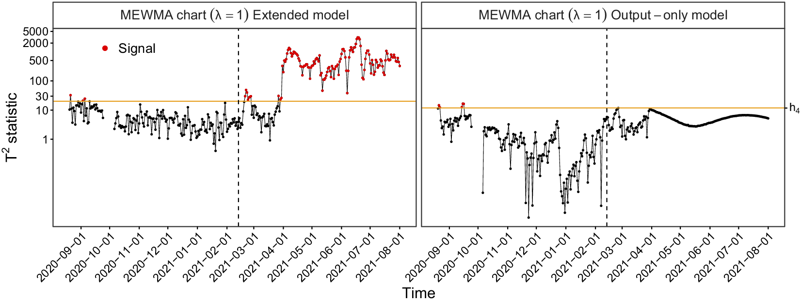
Figure 14. MEWMA Control chart for $ \lambda =1 $
on a logarithmic y-axis, using an extended functional model (left) and the output-only functional model (right) for the Sachsengraben viaduct.
$ \lambda =1 $
on a logarithmic y-axis, using an extended functional model (left) and the output-only functional model (right) for the Sachsengraben viaduct.
5. Concluding remarks
The modeling and monitoring methodology presented in this paper combines several parts of a structural health monitoring system in one unified framework (CAFDA-SHM). It is of high practical relevance, as it tackles important challenges in SHM. The discussed functional data approach offers the flexibility to model recurring daily and yearly patterns alongside environmental or operational influences in a highly adaptable and interpretable semiparametric manner. It can handle missing observations and effectively accounts for variations and correlations in the error process through functional principal components. Furthermore, FPCA extracts interpretable, data-based features, which are then utilized for monitoring within a sound statistical framework, thus providing a reliable basis for decision-making. Our real-world data analyses showed that CAFDA-SHM can be used for covariate adjustment and monitoring of different types of response variables: dynamic responses, as shown in Section 4.1, and quasi-static responses, as demonstrated in Section 4.2. It is hence planned to implement and test the methods presented in this article as part of a larger online SHM system (Kessler et al., Reference Kessler, Mendler, Klemm, Jaelani, Köhncke and Gündel2024).
Although the proposed modeling approach is an input–output method, it contains an output-only FPCA-based version as a particular case. The latter has advantages over existing approaches as it accounts for daily and yearly patterns typically ignored by common PCA-based methods. Utilizing state-of-the-art functional additive mixed models enables nonlinear modeling, as often needed in SHM. Our approach is flexible in handling diverse data types, from sparse and aggregated to high-resolution, dense data. Although the focus of this article was on concurrent models, the framework of functional additive mixed models includes various other options, such as historical functional effects or the common linear function-on-function approach (compare Appendix A).
Finally, there are three noteworthy limitations. First, if the error process becomes close to white noise, e.g., because the covariates’ explanatory power is very high, the functional approach no longer provides much of an advantage over a standard, non-functional response surface model. Second, in the functional additive mixed model, we implicitly assume that the error process and the functional random effects are (at least approximately) Gaussian. However, if outliers are present in the data (compare, e.g., Capezza et al., Reference Capezza, Centofanti, Lepore and Palumbo2024), an additional step to identify these outliers would need to be included in a preprocessing step in our framework. Third, the framework presented in this paper is designed for univariate functional responses. Future research will involve modeling multiple system outputs simultaneously, such as natural frequencies of multiple modes.
Data availability statement
The vibration, temperature, and relative humidity data for the railway bridge KW51 are available from Maes and Lombaert (Reference Maes and Lombaert2020). The strain and temperature data for the viaduct Sachsengraben are available from Bundesanstalt für Straßenwesen (BASt) (2023). The source code for reproducing the main results of this paper is available at https://github.com/wittenberg/CAFDA-SHM_code.
Software
The main analysis used the statistical software R (R Core Team, 2023). In addition, functions from the following R packages were used. Some functions from the funData (Happ-Kurz, Reference Happ-Kurz2020) were used to generate the artificial data. The functional additive (mixed) modeling was carried out with mgcv (Wood, Reference Wood2017). Functional principal component analysis utilized refund (Goldsmith et al., Reference Goldsmith, Scheipl, Huang, Wrobel, Di, Gellar, Harezlak, McLean, Swihart, Xiao, Crainiceanu and Reiss2022). The control limits of the MEWMA control chart were calculated using the spc R package (Knoth, Reference Knoth2022), and the piecewise linear model was trained using the segmented R package (Muggeo, Reference Muggeo2008).
Acknowledgements
We thank three anonymous reviewers, the editor-in-chief, and the executive editor for their helpful comments on an earlier manuscript version. We thank Sven Knoth for his advice on the control charts.
Author contribution
Conceptualization: A.M., J.G., and P.W. Data curation: L.N. and P.W. Formal analysis: L.N. and P.W. Funding acquisition: J.G. Methodology: J.G. and P.W. Project administration: J.G. Resources: J.G. Software: P.W. Supervision: A.M. and J.G. Validation: L.N. and P.W. Visualization: P.W. Writing—original draft: J.G. and P.W. Writing—review and editing: A.M. J.G. L.N. and P.W. All authors approved the final submitted draft.
Funding statement
This research is funded by dtec.bw—Digitalization and Technology Research Center of the Bundeswehr. dtec.bw is funded by the European Union—NextGenerationEU. We thank the hpc.bw team for their support within the joint dtec.bw project “HPC for semi-parametric statistical modeling on massive datasets.”
Competing interests
The authors declare none.
Ethical standard
The research meets all ethical guidelines, including adherence to the legal requirements of the study country.
Appendix
A. Further modeling options
This Section provides an overview of various modeling options beyond the models discussed in the main paper. All models considered in Sections 2, 3, 4.1, and 4.2 were so-called concurrent models, where it is assumed that the system output at time $ t $
is influenced by covariate
$ t $
is influenced by covariate $ z $
measured at the same time
$ z $
measured at the same time $ t $
only. This makes sense for covariates such as the temperature of the structure itself, as available for the KW51 bridge and the Sachsengraben viaduct. However, if only ambient temperature is given, it seems more reasonable to assume that the temperature over the recent past, let us say three hours, is relevant. Appropriate models can be specified through so-called historical (functional) effects.
$ t $
only. This makes sense for covariates such as the temperature of the structure itself, as available for the KW51 bridge and the Sachsengraben viaduct. However, if only ambient temperature is given, it seems more reasonable to assume that the temperature over the recent past, let us say three hours, is relevant. Appropriate models can be specified through so-called historical (functional) effects.
-
• In the simplest case of a linear effect that does not change over the day, we have
where
$$ {u}_j(t)=\dots +{\int}_0^h\beta (s){z}_j\left(t-s\right) ds+\dots, $$
$ h $
denotes the time limit to look into the past, e.g., three hours. Typically, it is recommended to choose a rather large value here because, if
$ z $
in that time region is not relevant for
$ u $
anymore,
$ \beta (s) $
will be fit to tend towards zero for
$ s\to h $
(given there is enough data available to learn from).
-
• If the effect of
$ z $
is allowed to change over the course of the day
$ {\int}_0^h\beta (s){z}_j\left(t-s\right) ds $
turns into
$ {\int}_0^h\beta \left(s,t\right){z}_j\left(t-s\right) ds $
. -
• In the nonlinear setting, we have
$ {\int}_0^hf\left({z}_j\left(t-s\right),s\right) ds $
if the (historical) effect is constant across
$ t $
(i.e., the course of the day) and
$ {\int}_0^hf\left({z}_j\left(t-s\right),s,t\right) ds $
otherwise.


All those models fit into the framework of functional additive mixed models as well. Instead of the historical functional effects, we could also write
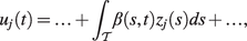 $$ {u}_j(t)=\dots +{\int}_{\mathcal{T}}\beta \left(s,t\right){z}_j(s) ds+\dots, $$
which is typically denoted as “linear function-on-function regression.” In fact, this is the most popular model for function-on-function regression, and, e.g., used by Centofanti et al. (Reference Centofanti, Lepore, Menafoglio, Palumbo and Vantini2021). The corresponding nonlinear/smooth version would be
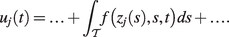 $$ {u}_j(t)=\dots +{\int}_{\mathcal{T}}f\left({z}_j(s),s,t\right) ds+\dots . $$
However, both models do not seem sensible approaches for SHM data as considered here because “future” observations $ {z}_j(s) $
, with
$ {z}_j(s) $
, with $ s>t $
, would be allowed to affect “present”
$ s>t $
, would be allowed to affect “present” $ {u}_j(t) $
.
$ {u}_j(t) $
.


 Open access
Comments
No Comments have been published for this article.