2.1. Compression algorithms

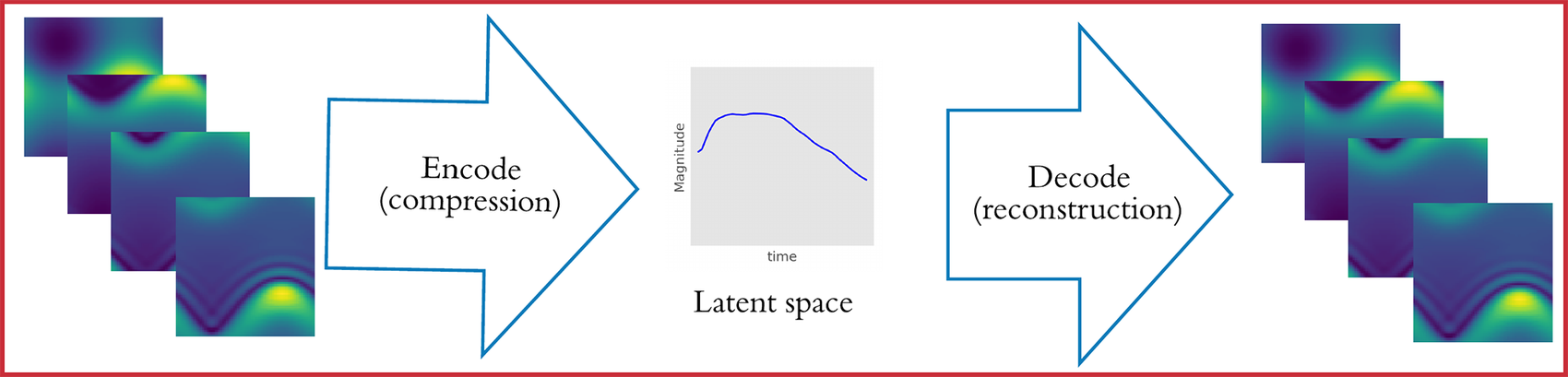
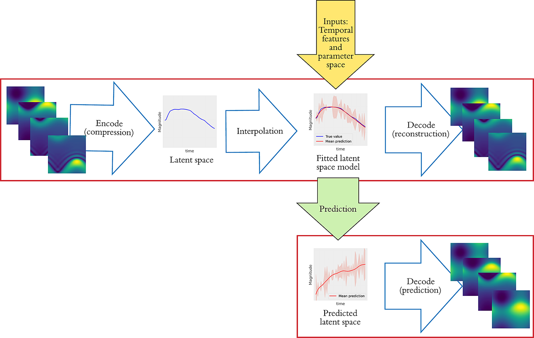
We focus on three different compression algorithms: PCA, CAE, and VAEs. In the context of CFD, a simulation involves the numerical solution of a set of differential equations that usually requires considerable computational resources (particularly if the simulations are spatio-temporal and solved in 3D space). A set of simulations is fed into one of the aforementioned ML algorithms in the form of images (frames that correspond to simulation timestamps). The information from the simulations is compressed and summarized in the form of the latent space, where it can be further manipulated and analyzed. Subsequently, the decompression portion of the algorithm can be used to reconstruct the original space. The whole process is shown in Figure 1.

Figure 1.

Schematic of reduced-order modeling. Spatio-temporal outputs of a simulation (left) are being fed into an encoder and output a latent space (middle). The reconstruction of the original system (right) is the output of the decoder that uses as input the aforementioned latent space. Lower panel shows the interpolation and forecasting in the latent space for reconstruction.

2.1.1. Principal component analysis

The PCA is a numerical method used to decompose a random vector field $ \mathbf{u}\left(\mathbf{d},t\right) $ (in which $ \mathbf{d} $ and $ t $ denote space, which in turn can be represented by an appropriate coordinate system, and time, respectively). Following the decomposition step, a new basis is created where the new variables are linear combinations of the originals such that the explainable system variance is maximized. The $ {n}_r $ -dimensional latent space is created by selecting the $ {n}_r $ first components and discarding the rest.

To carry out a PCA, we first take $ p $ temporal snapshots of the field $ \mathbf{s} $ , which for $ n $ spatial elements yields the matrix $ \mathbf{S} $ :

$$ \mathbf{S}=\left[\begin{array}{ccc}u\left({d}_1,{t}_1\right)& \cdots & u\left({d}_n,{t}_1\right)\\ {}\cdots & \cdots & \cdots \\ {}u\left({d}_1,{t}_p\right)& \cdots & u\left({d}_n,{t}_p\right)\end{array}\right]. $$

Then, we compute the covariance matrix $ \mathbf{C} $ of $ \mathbf{S} $ as:

$$ \mathbf{C}=\frac{1}{p-1}{\mathbf{U}}^T\mathbf{U}, $$

where $ \mathbf{U} $ is an orthogonal matrix and consequently the eigenvalue diagonal matrix $ \Lambda =\operatorname{diag}\left\{{\lambda}_1,\dots, {\lambda}_n\right\} $ , where $ {\lambda}_1\le \dots \le {\lambda}_n $ and the corresponding eigenvector matrix $ W $ are derived from:

$$ \mathbf{CW}=\mathbf{W}\Lambda . $$

Finally, the PCA basis is given by:

$$ \theta =\mathbf{UW}, $$

and choosing the first $ {n}_r $ columns of $ \theta $ results in the creation of an $ {n}_r $ -dimensional latent space. The main advantage of the PCA is its simplicity and ease of computation, but the quality of the results is not necessarily equivalent to that of more sophisticated methods.

2.1.2. Convolutional autoencoders

Autoencoders are classes of neural network algorithms used primarily for unsupervised learning purposes, such as dimensionality reduction, data generation, and feature learning. Their structure is based on a bottleneck that combines two individual components: the encoder, which is a neural network that passes the input through layers that consist of a decreasing number of neurons, up until the bottleneck, where it outputs the latent space; and the decoder, which has the opposite architecture, uses the latent space as input and aims to reconstruct the original data by minimizing the reconstruction error. For this work, we use CAE, which is a class of autoencoders that includes layers with convolutions (LeCun et al., Reference LeCun and Bengio1995), that is, a set of filters that extract specific features from images. The output $ {y}_{\mathrm{ijk}} $ of a typical neuron in a convolutional layer has the form:

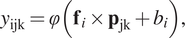$$ {y}_{\mathrm{ijk}}=\varphi \left({\mathbf{f}}_i\times {\mathbf{p}}_{\mathrm{jk}}+{b}_i\right), $$

where $ \varphi $ is an activation function, $ {\mathbf{f}}_i $ is a single filter, $ {\mathbf{p}}_{\mathrm{jk}} $ is a patch of data that shifts according to the dimensions $ j $ and $ k $ , and $ {b}_i $ is a bias term. In practice, the convolutional layers learn different features and patterns from the original data, particularly useful in image processing.

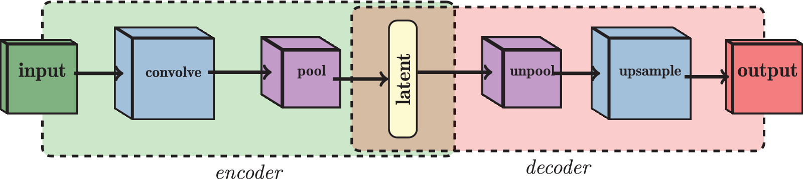
Another type of layer found in a convolutional neural network (CNN) is a pooling layer, which generally follows one (or more than one) convolutional layer with the aim of subsampling and summarizing the information from the filters. In a typical CNN, the continuous alternation of convolutional and pooling layers is how a neural network can extract high- and low-level features. In CAEs, the decoder comprises the opposite structure to that of the encoder. Instead of the convolutional and pooling layers, it consists of upsampling and unpooling layers respectively, where it produces an output of the same size as the input data using nearest-neighbor interpolation. A loss function such as the mean squared error (MSE) is then used during training in order to update the neural network’s weights in a manner that minimizes the reconstruction error between the input and the output. The general structure of the CAE with all the components described above is shown in Figure 2.

Figure 2.

Architecture of a convolutional autoencoder (CAE). The input frames are fed into the encoder, where convolutional (convolve) and pooling (pool) layers are used, in order to produce the latent space. The reverse scheme is used for the decoder, where unpooling (unpool) and upsampling (upsample) layers are used to produce an output as similar as possible to the original input.

2.1.3. Variational convolutional autoencoders

A similar class of algorithms is VAEs (Kingma and Welling, Reference Kingma and Welling2013). The main difference between these and their conventional convolutional counterparts is that the latent space is provided in the form of a probability distribution, usually a Gaussian. In practice this representation acts as regularization for the latent space, which can be particularly beneficial when quality of the data is poor. In order to reconstruct the input, a sample is drawn from the latent space distribution.

The encoder and decoder of a VAE can be described as the functions $ q\left(\mathbf{z}|\mathbf{x}\right) $ and $ p\left({\mathbf{x}}^{\prime }|\mathbf{z}\right) $ respectively, where $ \mathbf{x} $ is the input, $ \mathbf{z} $ is the latent space and $ {\mathbf{x}}^{\prime } $ is the output. The latent space follows a Gaussian distribution $ \mathbf{z}\sim \mathcal{N}\left(\mu, {\sigma}^2\right) $ due to the Kullback–Leibler divergence (KL divergence) $ {D}_{\mathrm{KL}}\left(q\left(\mathbf{z}|{\mathbf{x}}_i\right)\Big\Vert p\left(\mathbf{z}|{\mathbf{x}}_i\right)\right) $ . The VAE loss has two components: the reconstruction loss (similar to the CAE) and the KL loss,

$$ {E}_{q\left(\mathbf{z}|{\mathbf{x}}_i\right)}\left[\log p\left({\mathbf{x}}_i|\mathbf{z}\right)\right]-{D}_{\mathrm{KL}}\left(q\left(\mathbf{z}|{\mathbf{x}}_i\right)\Big\Vert p\left(\mathbf{z}|{\mathbf{x}}_i\right)\right), $$

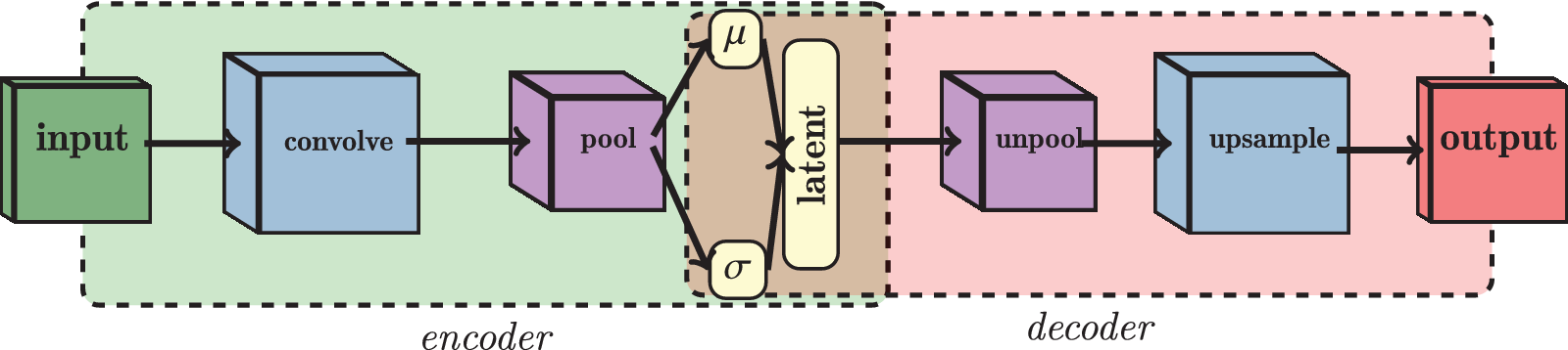
which ensure that the output is as similar as possible to the input and that the distribution of $ z $ is Gaussian, respectively. The practical difference between a CAE and a VAE is that, as shown in Figure 3, the output of the VAE encoder consists of two vectors $ \mu $ and $ \sigma $ . Given $ \varepsilon \sim N\left(0,I\right) $ , where $ I $ is the identity matrix we can use the reparameterization trick (Kingma and Welling, Reference Kingma and Welling2013) and write the latent space as $ z=\mu +\sigma \varepsilon $ , which is a form suitable for training. For the implementation of the autoencoders we use the TensorFlow package (Abadi et al., Reference Abadi, Agarwal, Barham, Brevdo, Chen, Citro, Corrado, Davis, Dean and Devin2016).

Figure 3.

Architecture of a VAE. It is similar to the CAE equivalent, with the additional assumption that the latent space is a set of multivariate Gaussian distributions, and can be described as $ z\sim N\left(\mu, {\sigma}^2\right) $ .

2.2. Interpolation algorithms

The enhanced ROM methodology that includes the interpolation step is shown in Figure 4. After we derive the latent space (in the same manner as in Section 2.1), we use it as input for an interpolation algorithm. The new model can be used for predictions with new sets of parameters, while the output can be further assessed and transformed back to the original space through the decoder.

Figure 4.

Schematic of the enhanced reduced-order modeling which features additional steps to Figure 1 involving interpolation of the latent space and (if required) prediction for new parameters. The outputs are fed into the decoder for transformation back to the original space.

There are various advantages underlying latent space interpolation. Specifically, the one that we primarily focus on in this work is the ability to interpolate and extrapolate in the parameters of interest. This is an important advantage for multiphase flow applications since new simulations can be computationally costly, and, therefore, the ability to relocate this problem into the low-dimensional latent space, where predictions are easily performed, can allow for predictions, based on sets of parameters, even when data are not available. Other advantages that were explored by Maulik et al. (Reference Maulik, Botsas, Ramachandra, Mason and Pan2021a) include interpolation in time, which can lead to finer temporal resolutions, increased interpretablility since the interpolation algorithm provides valuable visualizations of the latent space that can show the quality of the compression; and, finally, in the case where the interpolation algorithm is a GP, uncertainty quantification is also possible.

2.2.1. Gaussian processes

GPs (Rasmussen and Williams, Reference Rasmussen and Williams2006) are generalizations of multivariate Gaussian distributions with infinite-dimensional space and a popular choice for regression (Williams and Rasmussen, Reference Williams and Rasmussen1996) due to their versatility; the method is known as Gaussian process regression (GPR). We mainly focus on the mean prediction of a GP that corresponds to the maximum a posteriori estimate and use this as the decoder input.

Considering a mean function $ m\left(\mathbf{x}\right) $ equal to 0, a GP can be completely specified by its second-order statistics; therefore, a positive definite covariance function (otherwise known as a kernel) $ k\left(\mathbf{x},{\mathbf{x}}^{\prime}\right) $ is the only requirement. For a GPR model, we considered a GP $ f $ and noisy training observations $ \mathbf{y} $ of $ n $ datapoints $ \mathbf{x} $ derived from the true values $ f\left(\mathbf{x}\right) $ with additive i.i.d. Gaussian noise $ \varepsilon $ with variance $ {\sigma}_n^2 $ :

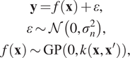(1) $$ {\displaystyle \begin{array}{c}\mathbf{y}=f\left(\mathbf{x}\right)+\varepsilon, \\ {}\varepsilon \sim \mathcal{N}\left(0,{\sigma}_n^2\right),\\ {}f\left(\mathbf{x}\right)\sim \mathrm{GP}\left(0,k\left(\mathbf{x},{\mathbf{x}}^{\prime}\right)\right),\end{array}} $$

where $ k\left(\cdot, \cdot \right) $ is the kernel. We obtain the complete GP specification by maximizing the marginal likelihood, which we can acquire by integrating the product of the Gaussian likelihood and the GP prior over $ f $ :

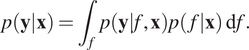(2) $$ p\left(\mathbf{y}|\mathbf{x}\right)={\int}_fp\left(\mathbf{y}|f,\mathbf{x}\right)p\left(f|\mathbf{x}\right)\hskip0.22em \mathrm{d}f. $$

For testing input $ {\mathbf{x}}_{\star } $ and output $ {\mathbf{f}}_{\star } $ , we derive the joint marginal likelihood:

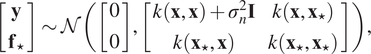$$ \left[\begin{array}{c}\mathbf{y}\\ {}{\mathbf{f}}_{\star}\end{array}\right]\sim \mathcal{N}\left(\left[\begin{array}{c}0\\ {}0\end{array}\right],\left[\begin{array}{cc}k\left(\mathbf{x},\mathbf{x}\right)+{\sigma}_n^2\mathbf{I}& k\left(\mathbf{x},{\mathbf{x}}_{\star}\right)\\ {}k\left({\mathbf{x}}_{\star },\mathbf{x}\right)& k\left({\mathbf{x}}_{\star },{\mathbf{x}}_{\star}\right)\end{array}\right]\right), $$

where $ \mathbf{I} $ is the identity matrix. Finally, by conditioning the joint distribution on the training data and the testing inputs, we derive the predictive distribution

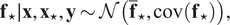(3) $$ {\mathbf{f}}_{\star}\mid \mathbf{x},{\mathbf{x}}_{\star },\mathbf{y}\sim \mathcal{N}\left({\overline{\mathbf{f}}}_{\star },\operatorname{cov}\left({\mathbf{f}}_{\star}\right)\right), $$

where $ {\overline{\mathbf{f}}}_{\star } $ and $ \mathit{\operatorname{cov}}\left({\mathbf{f}}_{\star}\right) $ are given by

(4) $$ {\displaystyle \begin{array}{c}{\overline{\mathbf{f}}}_{\star }=k\left({\mathbf{x}}_{\star },\mathbf{x}\right){\left[k\left(\mathbf{x},\mathbf{x}\right)+{\sigma}_n^2\mathbf{I}\right]}^{-1}\mathbf{y}\\ {}\operatorname{cov}\left({\mathbf{f}}_{\star}\right)=k\left({\mathbf{x}}_{\star },{\mathbf{x}}_{\star}\right)-k\left({\mathbf{x}}_{\star },\mathbf{x}\right){\left[k\left(\mathbf{x},\mathbf{x}\right)+{\sigma}_n^2\mathbf{I}\right]}^{-1}k\left(\mathbf{x},{\mathbf{x}}_{\star}\right).\end{array}} $$

We chose a single Matérn 3/2 kernel with lengthscale $ \mathbf{l} $ due to its versatility, flexibility, and smoothness. Specifically, we used the automatic relevance determination (ARD) extension Bishop (Reference Bishop2006), which incorporates a separate parameter for each input variable:

(5) $$ {\displaystyle \begin{array}{c}k\left(\mathbf{x},{\mathbf{x}}^{\prime}\right)=\left(1+\frac{\sqrt{3{\left(\mathbf{x}-{\mathbf{x}}^{\prime}\right)}^2}}{\mathbf{l}}\right)\exp \left(-\frac{\sqrt{3\left(\mathbf{x}-{\mathbf{x}}^{\prime}\right)}}{\mathbf{l}}\right).\end{array}} $$

Substitution of Equation (5) into Equation (4) yields:

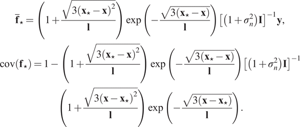(6) $$ {\displaystyle \begin{array}{c}{\overline{\mathbf{f}}}_{\star }=\left(1+\frac{\sqrt{3{\left({\mathbf{x}}_{\star }-\mathbf{x}\right)}^2}}{\mathbf{l}}\right)\exp \left(-\frac{\sqrt{3\left({\mathbf{x}}_{\star }-\mathbf{x}\right)}}{\mathbf{l}}\right){\left[\left(1+{\sigma}_n^2\right)\mathbf{I}\right]}^{-1}\mathbf{y},\\ {}\operatorname{cov}\left({\mathbf{f}}_{\star}\right)=1-\left(1+\frac{\sqrt{3{\left({\mathbf{x}}_{\star }-\mathbf{x}\right)}^2}}{\mathbf{l}}\right)\exp \left(-\frac{\sqrt{3\left({\mathbf{x}}_{\star }-\mathbf{x}\right)}}{\mathbf{l}}\right){\left[\left(1+{\sigma}_n^2\right)\mathbf{I}\right]}^{-1}\\ {}\left(1+\frac{\sqrt{3{\left(\mathbf{x}-{\mathbf{x}}_{\star}\right)}^2}}{\mathbf{l}}\right)\exp \left(-\frac{\sqrt{3\left(\mathbf{x}-{\mathbf{x}}_{\star}\right)}}{\mathbf{l}}\right).\end{array}} $$

During the reconstruction phase, we focus on the predictions that correspond to $ {\overline{\mathbf{f}}}_{\star } $ .

2.2.2. Deep Gaussian processes

A DGP (Damianou and Lawrence, Reference Damianou and Lawrence2013) is a hierarchical composition of conventional GPs. In a DGP model, the data is modeled as the output of a multivariate GP, the inputs to that GP are governed by another GP and so on. In practice, DGPs are multilayer generalizations of GPs. For the purposes of this work, we will use the doubly stochastic variational inference variant of the DGP (Salimbeni and Deisenroth, Reference Salimbeni and Deisenroth2017), according to which for $ L $ layers we derive the joint density:

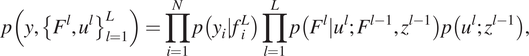(7) $$ p\left(y,{\left\{{F}^l,{u}^l\right\}}_{l=1}^L\right)=\prod \limits_{i=1}^Np\left({y}_i|{f}_i^L\right)\prod \limits_{l=1}^Lp\left({F}^l|{u}^l;{F}^{l-1},{z}^{l-1}\right)p\left({u}^l;{z}^{l-1}\right), $$

where $ {F}^0=x $ . In Equation (7), $ x $ and $ y $ are the $ n $ -dimensional data (inputs and outputs respectively), $ {F}^i $ are stochastic functions with GPs as priors, $ {f}_i^L $ is the output of the last layer, $ {z}^i $ is a set of inducing points at layer $ i $ , and $ {u}^i $ the corresponding inducing function values. Note that in this parameterization each of the GPs has a zero mean and the Gaussian noise is absorbed into the kernel. By assuming that the posterior $ q $ of $ {u}^i $ is factorized between layers and $ q\left({u}^i\right)\sim N\left({m}^i,{S}^i\right) $ , and after marginalizing the inducing variables of each layer, the marginal likelihood becomes:

(8) $$ q\left({\left\{{F}^l\right\}}_{i=1}^L\right)=\prod \limits_{i=1}^Lq\left({F}^l|{m}^l,{S}^l;{F}^{l-1},{Z}^{l-1}\right)=\prod \limits_{i=1}^LN\left({F}^l|{\overline{\mu}}^l,{\overline{\Sigma}}^l\right). $$

For new predictions the following equation applies:

$$ q\left({f}_{\ast}^L\right)=\frac{1}{V}\sum \limits_{v=1}^Vq\left({f}_{\ast}^L|{m}^L,{S}^L;{f}_{\ast}^{(v)\left(L-1\right)},{Z}^{L-1}\right), $$

where $ {f}_{\ast}^{(v)\left(L-1\right)} $ are $ V $ samples from Equation (8). For the implementation of GPs and DGPs we used the GPyTorch library (Gardner et al., Reference Gardner, Pleiss, Bindel, Weinberger and Wilson2018).

2.2.3. Long short-term memory networks

The long short-term memory networks (LSTMs) (Hochreiter and Schmidhuber, Reference Hochreiter and Schmidhuber1997) are a special case of recurrent neural networks (RNNs), a class of neural networks that account for sequential data, thus being particularly useful for problems with temporal components. LSTMs, specifically, use gated cells that allow information transfer from both the recent past (short-term memory) and the distant past (long-term memory). This is an advantage of LSTMs compared to other RNN variations in terms of the results quality and also presents a solution to practical problems such as vanishing gradients (very small gradients during backpropagation that can render neurons inactive). A typical LSTM cell consists of:

$$ {\displaystyle \begin{array}{c}\mathrm{forget}\ \mathrm{gate}:{f}_t={\sigma}_g\left({W}_f{x}_t+{U}_f{h}_{t-1}+{b}_f\right)\\ {}\mathrm{input}\ \mathrm{gate}:{i}_t={\sigma}_g\left({W}_i{x}_t+{U}_i{h}_{t-1}+{b}_i\right)\\ {}\mathrm{output}\ \mathrm{gate}:{o}_t={\sigma}_g\left({W}_o{x}_t+{U}_o{h}_{t-1}+{b}_o\right)\\ {}\mathrm{cell}\ \mathrm{input}:{\overline{c}}_t={\sigma}_c\left({W}_c{x}_t+{U}_c{h}_{t-1}+{b}_c\right)\\ {}\mathrm{cell}\ \mathrm{state}:{c}_t={f}_t\odot {c}_{t-1}+{i}_t\odot {\overline{c}}_t\\ {}\mathrm{hidden}\ \mathrm{state}:{h}_t={o}_t\odot {c}_t,\end{array}} $$

where $ t $ denotes the time, $ {x}_t $ is the input, $ {W}_{\ast } $ , $ {U}_{\ast } $ , and $ {b}_{\ast } $ are the weights of the input and recurrent connection matrices and bias terms of the quantity $ \ast $ respectively, $ \odot $ is the element-wise product, $ {\sigma}_g $ is the sigmoid function and $ {\sigma}_c $ is the hyperbolic tangent function.

2.3. Methodology summary

The main steps of the methodology are:

1. 1. Create realistic synthetic data-sets for different parameter values and time-steps.

2. 2. Feed the data into the dimensionality reduction techniques (PCA, CAE, and VAE) in order to derive a latent space (reduced order).

3. 3. Train an interpolation (regression) algorithm (GP, DGP, and LSTM) using the latent space, the associated parameters and time steps.

4. 4. Given the trained interpolation algorithm, we make predictions for new sets of parameters, that were not included in the original data creation. This leads to new values of the latent space.

5. 5. Feed the newly predicted latent space values into the inverse component of the dimensionality reduction algorithm (decoding part). The result gives an approximation of a simulation for the parameters that were used in step 4 (and were omitted from step 1).

Note that the whole procedure described here is presented visually in Figure 4.

3.1. Advection–diffusion

Advection–diffusion equations expressed as

(9) $$ \frac{\partial c}{\partial t}+\overrightarrow{v}\cdot \overrightarrow{\nabla}c=D{\nabla}^2c $$

describe physical phenomena where mass, momentum, and energy are transported within a physical domain advectively by bulk motion and diffusively in response to differences in chemical potential and/or temperature. Here, $ c $ is a concentration, $ D $ is a constant diffusion coefficient, $ \overrightarrow{v}=\left({v}_x\left(x,y\right),{v}_y\left(x,y\right)\right) $ is the velocity field, and $ \overrightarrow{\nabla} $ denotes the gradient operator. Note that for a constant velocity, $ {U}_c $ , and an appropriate characteristic length scale, $ {L}_c $ , one can scale space and time on $ {L}_c $ and $ {L}_c/{U}_c $ , respectively, to arrive at

(10) $$ \frac{\partial c}{\partial t}+\frac{\partial c}{\partial x}+\frac{\partial c}{\partial y}=\frac{1}{Pe}\left(\frac{\partial^2c}{\partial {x}^2}+\frac{\partial^2c}{\partial {y}^2}\right), $$

where $ Pe={U}_c{L}_c/D $ is a Péclet number.

To generate a characteristic advection–diffusion simulation data-set, we implement and solve Equation (10) using the framework of Bar-Sinai et al. (Reference Bar-Sinai, Hoyer, Hickey and Brenner2019) and Zhuang et al. (Reference Zhuang, Kochkov, Bar-Sinai, Brenner and Hoyer2020). For training purposes, we generate 20 simulations for different values of $ {Pe}^{-1} $ ranging between 0.05 and 0.15, representing a blob of inert tracer placed in a constant-velocity fluid field. For each simulation, 50 evenly spaced time-snapshots with $ 64\times 64 $ resolution are obtained to construct the full data-set. We split the simulations into 19 cases for training and 1 for testing, focusing on the extrapolation problem. The data are fed into the three algorithms presented in Section 2.1. We train the different compression algorithms for four degrees of freedom (DOF). For an extensive analysis on how different DOF affect the result, we refer the reader to the experiment section in Maulik et al. (Reference Maulik, Botsas, Ramachandra, Mason and Pan2021a). For the encoders of the CAE and VAE we use five convolutional and pooling layers and an equal number of unpooling and upsampling layers for the decoders. We also train the data in mini-batches of four, and we use 1,000 epochs and early stopping based on a validation set that consists of 10% of the training data. We use TensorFlow (Abadi et al., Reference Abadi, Agarwal, Barham, Brevdo, Chen, Citro, Corrado, Davis, Dean and Devin2016) for autoencoder implementations. For the GPs we use an ARD Matérn 3/2 kernel with two-dimensional lengthscale (one dimension corresponds to the diffusion coefficient and the other to the temporal parameter). For the DGPs we use 128 inducing points, two layers, each of which comprises of a single GP with a Matérn 3/2 kernel. Finally, for the LSTM architecture, we use three cells with 50 neurons in each cell, mini-batches of size 32, early stopping based on 10% of the training data that are set aside, and a time window of 10 points for the forecasts, following a similar approach to Maulik et al. (Reference Maulik, Lusch and Balaprakash2021b). All the interpolation algorithms use the $ Pe $ value as an additional input to perform the latent space interpolation.

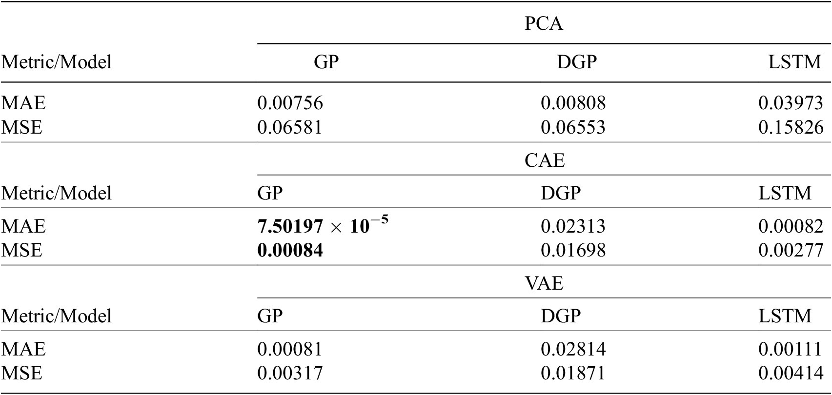
To assess the different methods, we use two metrics: the MSE and the mean absolute error (MAE). We remind the reader that output frames derived directly from the compression algorithms (in a typical ROM assessment fashion) are not possible to derive, since we make predictions for $ Pe $ values outside the training set. It is clear from Table 1 that PCA and DGP are consistently the worst performing of the compression and interpolation algorithms, respectively (with a few exceptions, such as DGP outperforming LSTM for the PCA case); the conclusion associated with PCA was one also reached by Maulik et al. (Reference Maulik, Botsas, Ramachandra, Mason and Pan2021a). As for the DGP conclusion, it appears that the additional complexity of using the DGP is unwarranted when applied to relatively small and simple data-sets, and that the corresponding model may become over-parameterized. Instead, the standard GP is flexible enough to capture the variability of the data obviating the need for a DGP. It is also unclear based on the results presented which of the two autoencoders and remaining interpolation algorithms performs better. The MAE favors all the LSTM variations, and specifically the CAE–LSTM combination, while the MSE is lower for the GP variations and especially VAE–GP, indicating that the LSTM offers lower average error and the GP fewer error spikes. The error values, however, are very small signifying the overall effectiveness of the methodology.

Table 1.

Evaluation metrics for the PCA, CAE, and VAE models for the advection–diffusion problem.

Note. The best performance for each metric (i.e., MAE and MSE) is highlighted in bold.

Abbreviations: CAE, convolutional autoencoder; DGP, deep Gaussian processes; GP, Gaussian process; LSTM, long short-term memory; MAE, mean absolute error; MSE, mean squared error; PCA, principal component analysis; VAE, variational convolutional autoencoders.

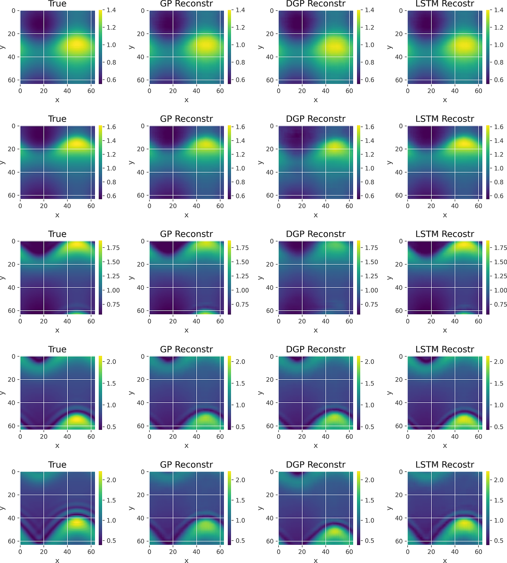
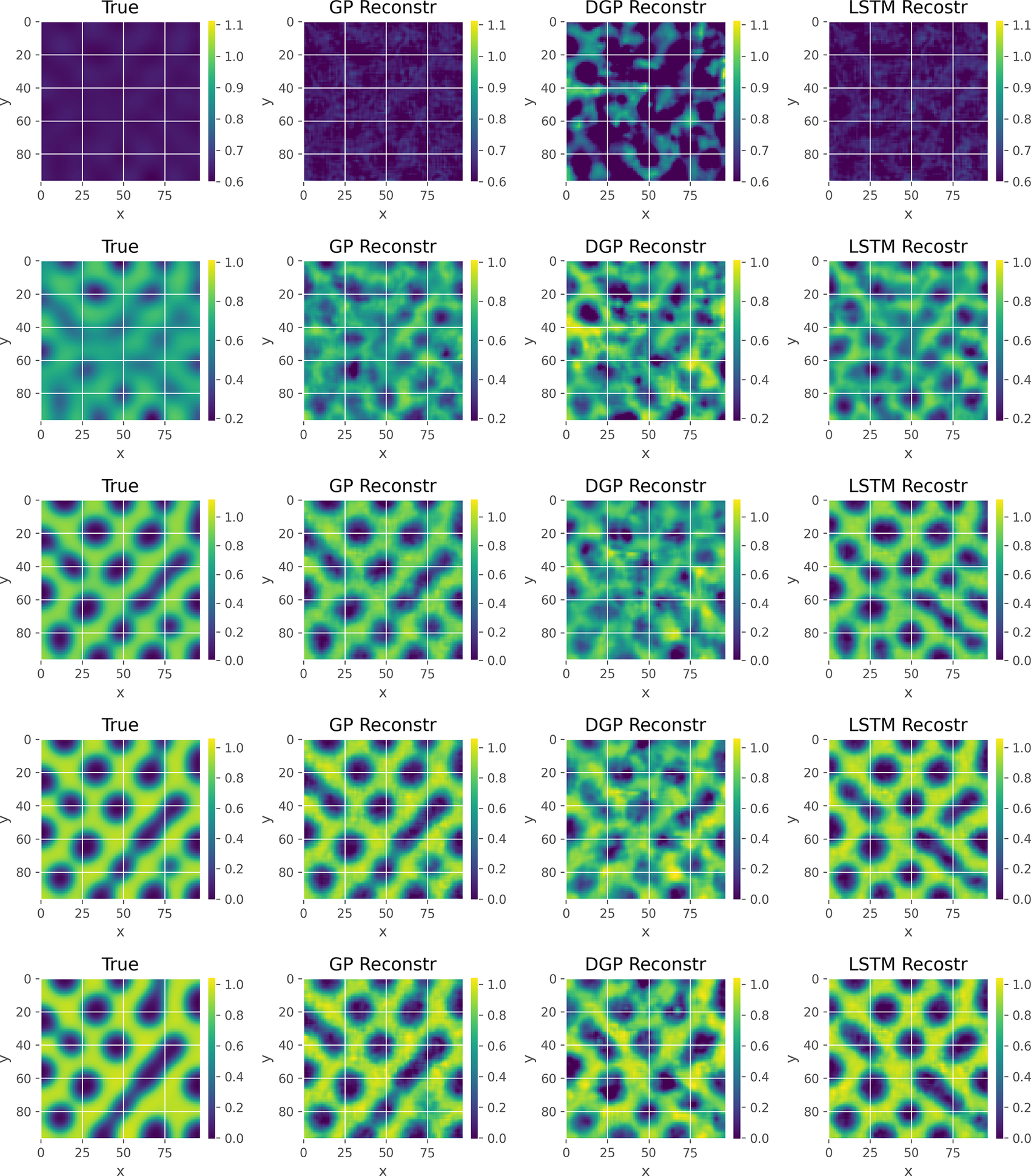
In Figures 5 and 6, we show indicative input frames (from top to bottom: 11, 21, 31, 41, and 50), along with the different VAE-based reconstructions and the corresponding residual plots, respectively. Specifically, the first column in Figure 5 corresponds to the true frames, the second to the GP reconstruction, the third to the DGP reconstruction, and the final to the LSTM reconstruction. Typically the true frames (left column) would not be available (nor required for the production of the two other columns), but here they are included for reference and model validation. The scaling is common for each row. Figure 6 uses the last three cases for the corresponding residuals. In order to show the differences among these plots we use flexible scaling. In terms of the actual frames we can see that the reconstruction is successful and it is hard to detect differences from the originals, even in the case of the DGP, which is the interpolation algorithm that performed more poorly, with some minor exceptions in the bottom frames. Regarding the residuals, we can see the similar error patterns generated, though, the scale makes it clear that the average error is larger for some of the frames in the GP and most in the DGP cases, when compared to the LSTM column.

Figure 5.

True and reconstructed frames for the concentration profiles of the VAE-related methods applied to the advection–diffusion problem. The rows correspond to time-steps 11, 21, 31, 41, and 50, respectively.

Figure 6.

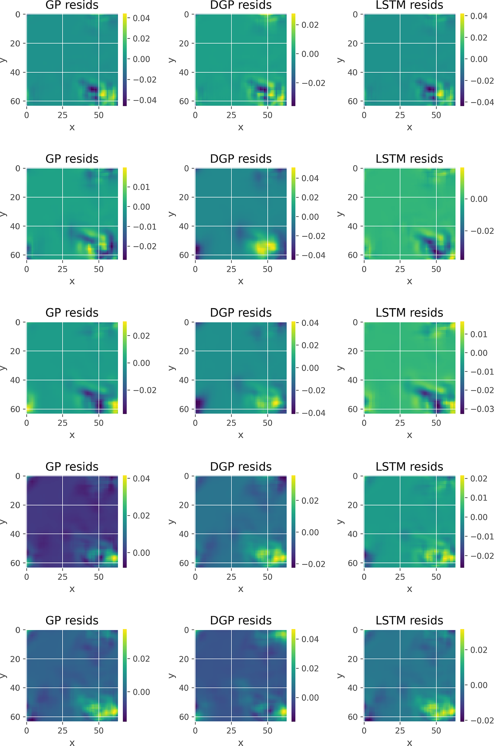
Residual concentration profile plots of the VAE-related methods applied to the advection–diffusion problem. The rows correspond to time-steps 11, 21, 31, 41, and 50, respectively.

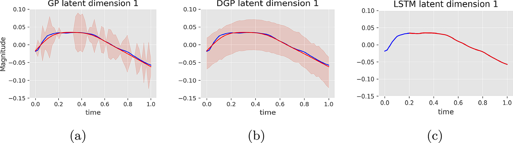
In Figure 7, we gain insights into the practical differences between the three interpolation algorithms by showing the corresponding representations of the first dimension of the latent space. The blue line shows the actual first dimension from the VAE latent space, the red line the mean for the GP-based algorithms for the first two and the output of the LSTM for the third, and the light red shading the confidence intervals around $ 2 $ standard deviations from the mean. Starting from the GP (Figure 7a) we can see a very good fit and an inconsistent uncertainty level. Generally, the uncertainty is narrower close to the times where data are available and wider everywhere else. The DGP case (Figure 7b) shows a very similar mean result, but the over-parameterization resulted to a wide uniform credible interval along the time axis. Finally, the LSTM (Figure 7c) shows an almost perfect fit to the latent space. The missing line before $ t=0.2 $ of the plot corresponds to the timewindow of $ 10 $ points that is required for the forecast.

Figure 7.

Comparison of the interpolation techniques; GP in (a), DGP in (b), and LSTM in (c), in the latent space for advection–diffusion.

The computational cost for all the algorithms examined in this section is shown in Table 2. The compression algorithm is run first and its cost is common for all relative pipelines regardless of the choice of the interpolation. PCA is almost instantaneous, while the autoencoders require a similar amount of time with each other. The time to solution for the interpolation algorithms differ based on the compression algorithm they follow, but the scale remains approximately the same. Specifically, LSTMs are consistently the fastest, followed by GPs, while DGPs are the slowest. It is worth noting that different parameterizations of the algorithms can potentially lead to significant differences with respect to computational costs, within each class of compression and interpolation.

Table 2.

Computational cost (in seconds) for all compression and interpolation algorithms.

Abbreviations: CAE, convolutional autoencoder; DGP, deep Gaussian processes; GP, Gaussian process; LSTM, long short-term memory; PCA, principal component analysis; VAE, variational convolutional autoencoder.

3.2. Falling films

We focus in this application on two-dimensional falling film flows, of importance to engineering applications including separation and heat removal units (Rohlfs et al., Reference Rohlfs, Rietz and Scheid2018). We apply the modeling framework of Scheid et al. (Reference Scheid, Ruyer-Quil and Manneville2006), which uses an averaged version of the Navier–Stokes equations together with Pade approximants; this yields a three-field equation system for the film thickness, $ h $ , and flow rates in the streamwise direction $ x $ , $ {q}^x $ , and spanwise one $ y $ , $ {q}^y $ , expressed by

(11) $$ \frac{\partial h}{\partial t}=-\frac{\partial {q}^x}{\partial x}-\frac{\partial {q}^y}{\partial y}, $$

(12) $$ \delta \frac{\partial {q}^x}{\partial t}=\delta \frac{\partial {\mathcal{I}}^{2D}}{\partial x}+\mathcal{G}\left(\frac{5}{6}h-\frac{5}{2{h}^2}\frac{\partial {q}^x}{\partial x}+\delta \frac{\partial {\mathcal{I}}^{3D}}{\partial x}+\eta \left[\frac{\partial {\mathcal{D}}^{2D}}{\partial x}+\frac{\partial {\mathcal{D}}^{3D}}{\partial x}\right]+\frac{5h}{6}\frac{\partial \mathcal{P}}{\partial x}\right), $$

(13) $$ \delta \frac{\partial {q}^y}{\partial t}=\delta \frac{\partial {\mathcal{I}}^{2D}}{\partial y}-\frac{5}{2{h}^2}\frac{\partial {q}^y}{\partial y}+\delta \frac{\partial {\mathcal{I}}^{3D}}{\partial y}+\eta \left[\frac{\partial {\mathcal{D}}^{2D}}{\partial y}+\frac{\partial {\mathcal{D}}^{3D}}{\partial y}\right]+\frac{5h}{6}\frac{\partial \mathcal{P}}{\partial y}, $$

where $ \mathcal{G}={\left[1-\left(\delta /70\right){h}^3\frac{\partial h}{\partial x}\right]}^{-1} $ , $ \mathcal{I} $ and $ \mathcal{D} $ represent a collection of terms related to inertia and viscous dissipation, defined in equations (B1b) and (B1c) in Scheid et al. (Reference Scheid, Ruyer-Quil and Manneville2006), and $ \mathcal{P}=-\zeta h+h\left(\frac{\partial^2h}{\partial {x}^2}+\frac{\partial^2h}{\partial {y}^2}\right) $ represents contributions to the pressure due to gravity and capillarity. The parameters $ \delta $ , $ \eta $ , and $ \zeta $ respectively represent the relative significance of inertia, gravity, and capillarity namely equations (2.9) and (2.10) in Scheid et al. (Reference Scheid, Ruyer-Quil and Manneville2006); the parameter $ \delta $ is referred to as a reduced Reynolds number.

Data were obtained from numerical solutions of Equations (11)–(13) simulated using a custom port of WaveMaker (Rohlfs et al., Reference Rohlfs, Rietz and Scheid2018) implemented in the Julia language (Bezanson et al., Reference Bezanson, Edelman, Karpinski and Shah2017). The general structure for this application has a significant degree of similarity with the one applied in Section 3.1, but with a few key differences: first, the simulations are generated based on the reduced Reynolds number $ \delta $ that takes 20 equi-spaced values in the range of 1–69. This is also the parameter used for the interpolation algorithms. Second, in this application we focus on the interpolation problem. Specifically, we use the sixth simulation (that corresponds to $ \delta =25.5 $ ) for testing and the rest for training. Finally, we use five DOF.

The metrics for all the results are shown in Table 3. Similar to the first advection–diffusion application, the PCA and the DGP underperform when compared to the other methods. For this data-set the combination of CAE and LSTM was the best performing based on both the MAE and the MSE metrics. As with the advection–diffusion application, finding differences between the frames for the interpolation algorithms paired with the CAE compression, and the true frames, which are included for reference, on the leftmost column of Figure 8 is difficult, regardless of the significant differences shown by the metrics. The only notable exception is the DGP reconstruction that shows slight deviations from the true film thickness. It is interesting to note that for all methods in Figure 9, and particularly the LSTM, the error structure in the upper frames (early times) seems random, whereas in the bottom frames (late times) we can clearly see the general structure of the film thickness. This indicates that it is easier for the methodology to reconstruct the frames from the beginning of the simulations (where all training simulations are similar) rather than the ending (where deviations among simulations are visibly different from each other due to the effect of the different reduced Reynolds numbers).

Table 3.

Evaluation metrics for the PCA, CAE, and VAE models.

Note. The best performance for each metric (i.e., MAE, MSE) is highlighted in bold.

Abbreviations: CAE, convolutional autoencoder; DGP, deep Gaussian processes; GP, Gaussian process; LSTM, long short-term memory; MAE, mean absolute error; MSE, mean squared error; PCA, principal component analysis; VAE, variational convolutional autoencoders.

Figure 8.

True and reconstructed frames of the film thickness for the CAE-related methods employed in the falling film problem. The rows correspond to time-steps 11, 21, 31, 41, and 50, respectively.

Figure 9.

Residual plots of the film thickness associated with the CAE-related methods used in the falling film problem. The rows correspond to time-steps 11, 21, 31, 41, and 50, respectively.

3.3. Multicomponent polymer precipitation

We now apply the analysis pipeline to polymer precipitation dynamics, of importance to engineering design problems in high-performance plastics and membrane systems. The complex dynamics and rich pattern formation were considered recently by Inguva et al. (Reference Inguva, Mason, Pan, Hengardi and Matar2020, Reference Inguva, Walker, Yew, Zhu, Haslam and Matar2021) (see also references therein) who used Cahn–Hilliard theory to model and simulate the spatio-temporal evolution of the emergent phase separation patterns; the relevant equations for a binary polymer blend are expressed by

(14) $$ \frac{\partial \phi }{\partial t}-\nabla \cdot \left(M\nabla \mu \right)=0, $$

where $ \phi $ represents the volume fraction of one of the polymers in the blend, $ M $ is a constant mobility parameter, and $ \mu $ is a generalized chemical potential, which can be derived from the variational derivative of the Gibbs free energy functional:

(15) $$ \mu =\frac{d f}{d\phi}-\lambda {\nabla}^2\phi; $$

here, $ f $ denotes the homogeneous contribution to the Gibbs free energy per monomer, which is a nonconvex function of $ \phi $ , and $ \lambda $ is a gradient free energy parameter. Numerical solutions of the above equations are obtained subject to Neumann conditions:

$$ {\displaystyle \begin{array}{l}\nabla \mu \cdot \mathbf{n}=0,\\ {}\nabla c\cdot \mathbf{n}=0,\end{array}} $$

in which $ \mathbf{n} $ is the outward-directed boundary normal.

For training purposes, we generate 20 simulations based on values of $ \lambda $ within the range 0.01–0.0575, which is also the parameter used for the interpolation algorithms. We use the python API of the FEniCS project Alnæs et al. (Reference Alnæs, Blechta, Hake, Johansson, Kehlet, Logg, Richardson, Ring, Rognes and Wells2015) for the simulations. An interesting complication comes from the fact that the simulator provides results in the form of $ 97\times 97 $ frames, which is not convenient for the standard structure of the autoencoders, since 97 is not a number that can be achieved with the up-sampling layers. This gives us the opportunity to examine how to address the issue of arbitrarily-shaped data. We tackle this with a zero padding that transforms the inputs to $ 128\times 128 $ frames. Once again, we are concerned with extrapolation, attempting to reconstruct the frames that correspond to the last $ \lambda $ value, and use five DOF. All the hyper-parameters of the compression and interpolation algorithms remain the same.

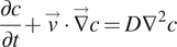
According to the results presented in Table 4, the best performing combination is the CAE paired with the GP. Both the MAE and the MSE indicate significant improvement from the other compression and interpolation algorithms. The zero padding seems to affect the VAE negatively, which struggles to deal with the abrupt transitions between the zero-padded sections and the actual frames possibly due to the distributional aspect of the algorithm. The unusual structure of the data is not easy to capture as shown in Figure 10, where all the interpolation algorithms are shown for the CAE case. Note that the true volume fraction frames are included for reference. It is hard to distinguish anything in the earlier frames, mainly due to the common scaling and the fact that the DGP seems to be deviating significantly. In the frames that correspond to late times, we can observe the GP-reconstructed frames having some minor deviations from their true counterparts, but generally being able to capture the correct space of the circular features, while the other two methods deviate significantly.

Table 4.

Evaluation metrics for the PCA, CAE, and VAE models.

Note. The best performance for each metric (i.e., MAE and MSE) is highlighted in bold.

Abbreviations: CAE, convolutional autoencoder; DGP, deep Gaussian processes; GP, Gaussian process; LSTM, long short-term memory; MAE, mean absolute error; MSE, mean squared error; PCA, principal component analysis; VAE, variational convolutional autoencoders.

Figure 10.

True and reconstructed frames for the volume fraction of the CAE-related methods used in the polymer precipitation problems. The rows correspond to time-steps 11, 21, 31, 41, and 50, respectively.

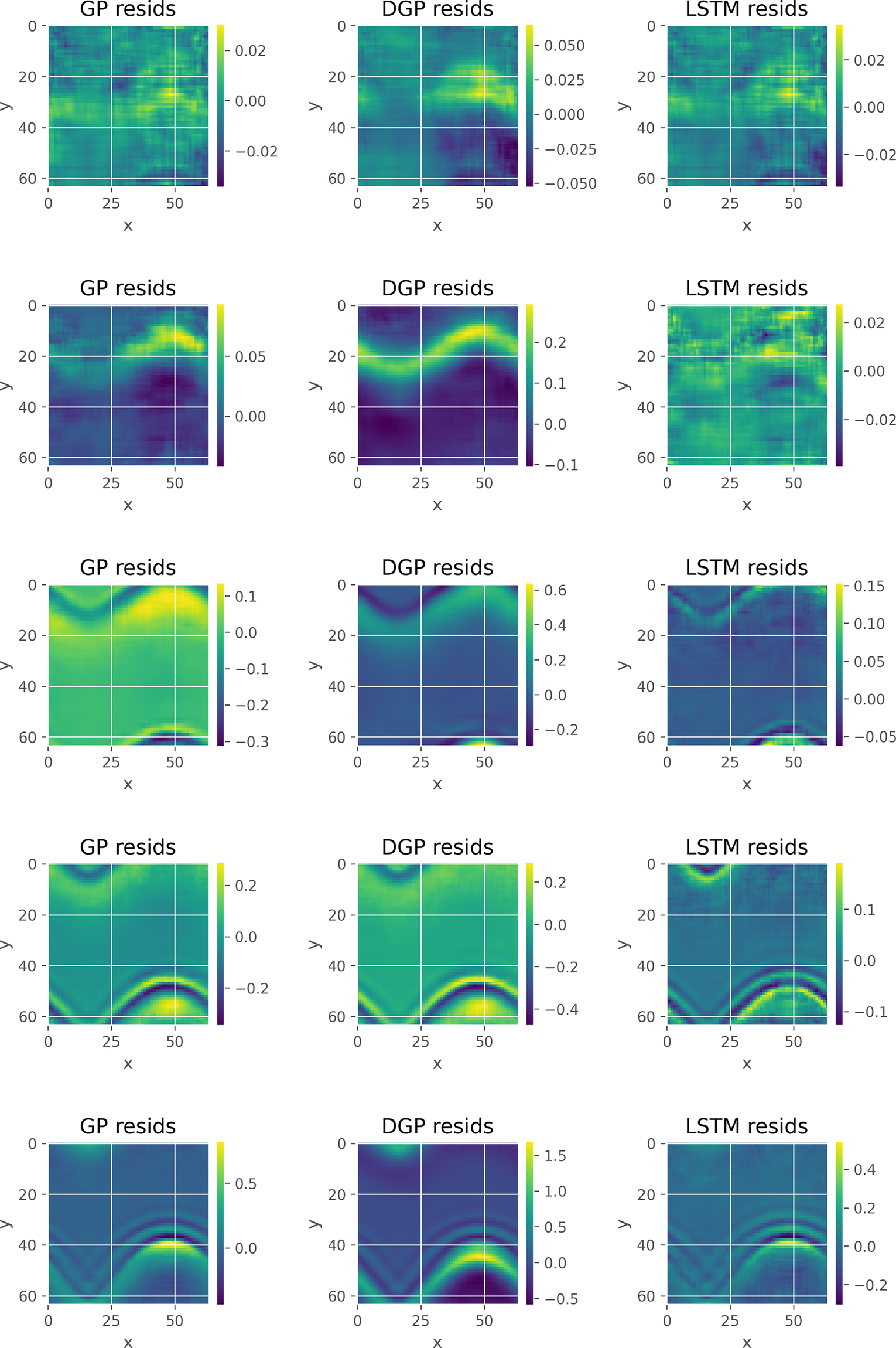
Finally, in Figure 11 we do not observe any specific pattern in the errors, which is expected from the structure of the data, but we can clearly see that the level of the errors is considerably lower for the late time frames in the GP case when compared to the other two.

Figure 11.

Residual volume fraction plots of the CAE-related methods in the polymer precipitation problems. The rows correspond to time-steps 11, 21, 31, 41, and 50, respectively.