

1 Introduction
Education contains a wealth of linked data whose key value lies in its connections. Existing processes underscore the value in exploring these relationships at a variety of scales: the mapping of prerequisite linkages across courses can identify gaps, overlaps and pathways in a curriculum redesign (Novak & Gowin Reference Novak and Gowin1984; Jenkins & Cho Reference Jenkins and Cho2013; Bailey et al. Reference Bailey, Jaggars and Jenkins2015), the linking of learning outcomes to educational resources is a necessary ingredient in designing adaptive learning systems, and the mapping of concepts in a concept map is a valuable exercise for instructional designers (Turns et al. Reference Turns, Atman and Adams2000; Jacobs Reference Jacobs2010). In evidence-based frameworks, studying linkages within and across learning processes are critical to informing instructional methods and changes in student knowledge (Koedinger et al. Reference Koedinger, Corbett and Perfetti2012). By analyzing the linkages within connected data, we can move toward learning engineering (Saxberg Reference Saxberg2017) and better design educational experiences (Novak & Gowin Reference Novak and Gowin1984; Carstensen & Bernhard Reference Carstensen, Bernhard, Björkqvist, Edström, Hugo, Kontio, Roslöf, Sellens and Virtanen2016).
Educational mapping is the process of analyzing an educational system to identify entities, relationships and attributes. Current mapping processes in education (such as curriculum mapping and concept mapping) typically represent data in forms that do not support scalable analysis. In particular, highly connected data are often represented in implicit forms where relationships within the data appear as flattened attributes of the entities they link (Guarino Reference Guarino1992). This lack of a first-class representation results in loss of information and forces ad hoc mechanisms to analyze connections in the system (Artale et al. Reference Artale, Franconi, Guarino and Pazzi1999)Footnote 1 . For example, a curriculum map is typically represented as a table, with topics or courses (the ‘entities’) listed in the rows of the table. Related data such as assessments, standards addressed, instructor, etc. are listed in the columns of the table. In this tabular representation, each row is recognized as an entity and given a first-class representation. However, an entity’s relationships are implicitly defined – flattened into column attributes of that row and thus not specified as first-class objects in their own right. This way of representing information means that analysis algorithms must be written in case-specific manner, requiring a potentially different analysis code for each new dataset. While acceptable for the one-off study, this manual approach does not scale to large or dynamic data sets, nor does it provide a structured foundation for visualization and analytics.
In this paper, we provide a structured scalable model on which to conduct educational mapping. We propose a network-based approach to modeling highly connected educational data. Network models are used in many fields to model entities and the relationships between them. Examples include social and organizational networks (Degenne & Forsé Reference Degenne and Forsé1999; Carrington et al. Reference Carrington, Scott and Wasserman2005; Lazer et al. Reference Lazer, Pentland, Adamic, Aral, Barabasi, Brewer, Christakis, Contractor, Fowler, Gutmann, Jebara, King, Macy, Roy and Van Alstyne2009; Clauset et al. Reference Clauset, Arbesman and Larremore2015), biological networks (Barabasi & Oltvai Reference Barabasi and Oltvai2004; Pujol et al. Reference Pujol, Mosca, Farrés and Aloy2010), and transportation networks (Bell & Lida Reference Bell and Lida1997). A primary strength of network models lies in their ability to explicitly represent relationships as first-class objects instead of as derived properties of other objects in the model. In the curriculum map example described above, a network model would explicitly represent as entities the topics, courses, assessments, standards, instructors, etc., and it would also explicitly represent the various relationships among these different kinds of entities. The reader could imagine multiple tables or spreadsheets listing all of these entities and all these relationships – while it might appear that the network model is a less compact representation than the traditional table, in fact this expanded representation is far more flexible and scalable. In this paper, we make the case that such a modeling approach is essential for representing, visualizing and analyzing educational data at scale. Scalable modeling is particularly important if the promise of learning analytics and educational analytics is to be fully unlocked (Campbell & Oblinger Reference Campbell and Oblinger2007; Siemens & Long Reference Siemens and Long2011). To motivate from concrete examples, we consider three use cases highly relevant in educational analytics – curriculum mapping, accreditation mapping and concept mapping – and we present an approach to formally model and analyze the corresponding data sets as a network.
2 Network models for education
In this section we first introduce some basic concepts of network modeling and graph theory. We then present three educational network models: a curriculum mapping model, an accreditation mapping model, and a concept mapping model. For each, we define the elements of the network model and discuss how the tools of graph theory can provide analysis and design of educational structures at different scales.
2.1 Basic concepts of network modeling
A graph structure $G$
, notionally portrayed in Figure 1, consists of a set of vertices and edges between vertices. Vertices represent entities in a system, and edges between vertices represent relationships between entities. For example, in a curriculum map the entities might be topics, courses, assessments, standards, schedule information and/or students. Relationship edges might represent information such as which topics are covered in each course, which courses a particular student has completed, which assessments relate to which topics and so on. Explicit modeling of these relationships in the graph structure unlocks the ability to perform scalable analyses on the dataset, such as a pathway analysis of topics to which each student has been exposed and the student’s associated level of competency for each topic. Such an analysis can be invaluable in student advising and career planning. Yet it is infeasible in current mapping processes where tabular models flatten relationships into implicit representations.
$G$
, notionally portrayed in Figure 1, consists of a set of vertices and edges between vertices. Vertices represent entities in a system, and edges between vertices represent relationships between entities. For example, in a curriculum map the entities might be topics, courses, assessments, standards, schedule information and/or students. Relationship edges might represent information such as which topics are covered in each course, which courses a particular student has completed, which assessments relate to which topics and so on. Explicit modeling of these relationships in the graph structure unlocks the ability to perform scalable analyses on the dataset, such as a pathway analysis of topics to which each student has been exposed and the student’s associated level of competency for each topic. Such an analysis can be invaluable in student advising and career planning. Yet it is infeasible in current mapping processes where tabular models flatten relationships into implicit representations.
In the graph structure, an edge is assigned text and numeric attributes, such as name, directionality, cost and weighting of the relationship. A vertex is assigned text and numeric attributes that represent information on the entity, including its name and other relevant properties. For a directed edge, the relationship applies only in one direction – the direction of the edge matters and is indicated visually with an arrow. For example, Course B may require Course A as a prerequisite. This would be represented as a directed edge pointing from Course A to Course B. An undirected edge is bidirectional – the relationship applies in both directions. For example, a topic may be related to another topic without any sense of ordering. Visually, this undirected edge is typically indicated by no arrow. The words graph and network are often used interchangeably; in this paper we use the term graph when discussing the theory and methods of graph structures and the term network to describe a situational structure with real world data representation.
A graph structure $G$
with three vertices and two edges. The edge from vertex A to vertex C is directed, while the edge between vertex A and vertex B is undirected.
$G$
with three vertices and two edges. The edge from vertex A to vertex C is directed, while the edge between vertex A and vertex B is undirected.

Several basic concepts of graph theory will be useful in analyzing our educational network models. We summarize those concepts here (with a minimal level of mathematical detail) and refer the reader to the textbooks (Bondy & Murty Reference Bondy and Murty1976; Bollob’as Reference Bollobás1998; West Reference West2001) for more detailFootnote 2 .
The degree of a vertex is defined as the number of edges between the vertex and other vertices in the graph. The degree distribution of the graph $P(k)$
is the fraction of vertices in the graph with degree
$P(k)$
is the fraction of vertices in the graph with degree $k$
. When edges are directed, the analysis of a vertex’s degree accounts for directionality: the indegree of a vertex is defined as the number of incoming directed edges from other vertices, and the outdegree of a vertex is defined as the number of outgoing directed edges to other vertices. These notions will be useful, for example, when assessing how the content in an educational program relates to student learning outcomes, or when assessing how a particular student’s coursework addresses accreditation outcomes. These concepts will be illustrated further in the accreditation mapping and concept mapping examples presented later in this paper.
$k$
. When edges are directed, the analysis of a vertex’s degree accounts for directionality: the indegree of a vertex is defined as the number of incoming directed edges from other vertices, and the outdegree of a vertex is defined as the number of outgoing directed edges to other vertices. These notions will be useful, for example, when assessing how the content in an educational program relates to student learning outcomes, or when assessing how a particular student’s coursework addresses accreditation outcomes. These concepts will be illustrated further in the accreditation mapping and concept mapping examples presented later in this paper.
We will sometimes be interested in analyzing just a portion of the network model. The term subgraph of a graph $G$
is another graph formed from a subset of the vertices and edges of
$G$
is another graph formed from a subset of the vertices and edges of $G$
. In some cases, we analyze the pathways associated with a directed subgraph. A topological sort of this subgraph results in an ordering of its vertices where for every directed edge from a vertex
$G$
. In some cases, we analyze the pathways associated with a directed subgraph. A topological sort of this subgraph results in an ordering of its vertices where for every directed edge from a vertex $A$
to a vertex
$A$
to a vertex $B$
,
$B$
, $A$
is ordered before
$A$
is ordered before $B$
. We can visually draw this subgraph with vertices arranged according to increasing path length from a source vertex, as shown notionally in Figure 2. We can then assign a rank to each vertex in the subgraph, where the rank of vertex
$B$
. We can visually draw this subgraph with vertices arranged according to increasing path length from a source vertex, as shown notionally in Figure 2. We can then assign a rank to each vertex in the subgraph, where the rank of vertex $V$
is defined to be the length of the longest path from the source vertex to vertex
$V$
is defined to be the length of the longest path from the source vertex to vertex $V$
. This analysis is useful, for example, when considering the prerequisite relationships between courses. In that case, the maximum length of the pathway associated with a particular course represents the most constraining set of prerequisite requirements that the student must complete before they can take that course. This provides valuable information for student advising and degree planning. This will be illustrated further in the curriculum mapping examples presented later in this paper.
$V$
. This analysis is useful, for example, when considering the prerequisite relationships between courses. In that case, the maximum length of the pathway associated with a particular course represents the most constraining set of prerequisite requirements that the student must complete before they can take that course. This provides valuable information for student advising and degree planning. This will be illustrated further in the curriculum mapping examples presented later in this paper.
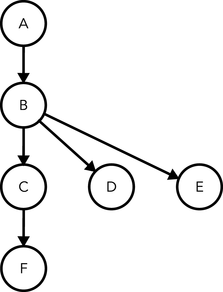
A directed graph with vertices arranged by assigned rank. Relative to the source vertex (vertex A): vertex A has a rank of 0; vertex B has a rank of 1; vertex C, vertex D and vertex E have a rank of 2; and vertex F has a rank of 3.
2.2 The curriculum mapping model
We define a curriculum mapping network model as follows. First, we define the different types of entities that reflect organization of the curriculum. As a first simple model to illustrate the ideas, consider a curriculum of a single institution, comprising a large number of courses arranged into departments. In this example, there are three different types of entities: a Course, a Department and an Institution. Categorizing the entities by different types will prove useful when we come to define relationships. Second, we define all the individual entities in the curriculum model: in this example, we define the individual courses, each of the departments, and the institution. Each one of these entities is modeled as a vertex in the curriculum network model. Third, each entity is assigned attributes. For example, a Course entity might have attributes that includes its name, course number, schedule information, website listing, etc. A Department entity might have attributes that includes its name, departmental code, website listing, department head, etc.
Next, we define different types of relationships among the entities. A basic curriculum model has three types of relationships: has-parent-of, has-prerequisite-of and has-corequisite-of. The has-parent-of relationship is a directed relationship that specifies organizational hierarchy in the curriculum. For example, we define has-parent-of relationships from a course to its parent department, and from a department to an institution. These relationships are modeled as directed edges between the appropriate vertices in the curriculum network model. The has-prerequisite-of and has-corequisite-of relationships are directed; they exist between courses to define prerequisite and corequisite relationshipsFootnote 3 . Again, these relationships are modeled as directed edges between the appropriate vertices in the curriculum network model.
To give a sense of scale of the model, if the curriculum comprises $n$
courses across
$n$
courses across $m$
departments and a single institution, then the total number of vertices in the network model is
$m$
departments and a single institution, then the total number of vertices in the network model is $n+m+1$
. If each course and each department has a single parent, there are
$n+m+1$
. If each course and each department has a single parent, there are $n+m$
parent grouping relationships. With
$n+m$
parent grouping relationships. With $r$
prerequisite relationships among classes and
$r$
prerequisite relationships among classes and $q$
corequisite relationships, there is a total of
$q$
corequisite relationships, there is a total of $n+m+r+q$
directed edges in the network model. For example, if an institution’s curriculum comprises 1000 courses across 25 departments with 1200 prerequisite relationships and 50 corequisite relationships, then our curriculum mapping network model has 1026 vertices and 2275 directed edges.
$n+m+r+q$
directed edges in the network model. For example, if an institution’s curriculum comprises 1000 courses across 25 departments with 1200 prerequisite relationships and 50 corequisite relationships, then our curriculum mapping network model has 1026 vertices and 2275 directed edges.
Figure 3 shows the curriculum model ontology corresponding to the network model described above. The left side of the figure shows the general ontology and the right side of the figure shows a concrete example. In this particular example ontology, a course is the most granular entity, but one could also define a more granular entity type, such as module (or some other unit of learning smaller than a full course). Similarly, one could introduce other units of organization, such as degree program, school, etc. One of the advantages of the network modeling approach is its flexibility to accommodate as many different types of entities and relationships as the modeler wishes to define for the particular use case.
A curriculum mapping model ontology. Left: the general ontology. Right: a concrete example.

This modeling approach can be used to model other, more complicated aspects of a curriculum. For example, sometimes multiple courses can fulfill a given prerequisite requirement. In this case, the basic has-prerequisite-of relationship does not capture the ‘or’ nature of the requirement; however, the network model can be extended to represent this situation. Consider a course $A$
that requires the student to complete
$A$
that requires the student to complete $\ell$
prerequisite courses chosen from a set
$\ell$
prerequisite courses chosen from a set ${\mathcal{C}}=\{c_{1},c_{2},\ldots ,c_{s}\}$
, where each
${\mathcal{C}}=\{c_{1},c_{2},\ldots ,c_{s}\}$
, where each $c_{i}$
is a course and
$c_{i}$
is a course and $s$
is the number of courses in the set of possibilities. Note that by definition,
$s$
is the number of courses in the set of possibilities. Note that by definition, $s\geqslant \ell$
, and if
$s\geqslant \ell$
, and if $s=\ell$
, we are in the simple case where there are no alternative options for a given prerequisite.
$s=\ell$
, we are in the simple case where there are no alternative options for a given prerequisite. ${\mathcal{C}}$
can then be modeled by a single vertex labeled OR. We attach a required-number attribute to the vertex with value
${\mathcal{C}}$
can then be modeled by a single vertex labeled OR. We attach a required-number attribute to the vertex with value $\ell$
. This required-number attribute specifies that a student must complete
$\ell$
. This required-number attribute specifies that a student must complete $\ell$
prerequisite courses from the specified set. The vertex representing course
$\ell$
prerequisite courses from the specified set. The vertex representing course $A$
is connected to the OR vertex via a has-prerequisite-of relationship. The OR vertex is further connected to the
$A$
is connected to the OR vertex via a has-prerequisite-of relationship. The OR vertex is further connected to the $s$
vertices representing the courses in the set
$s$
vertices representing the courses in the set ${\mathcal{C}}$
, via can-be relationships. This modeling is illustrated in Figure 4.
${\mathcal{C}}$
, via can-be relationships. This modeling is illustrated in Figure 4.
Capturing the situation of alternate prerequisite requirements by introducing an OR vertex and can-be relationship to the network model. Left: the general ontology. Right: a concrete example.
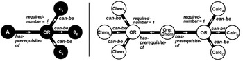
Note also that this model extends easily to the case of multiple ‘or’ requirements. For example, consider the case that an organic chemistry course (Org. Chem) has a prerequisite requirement that a student has completed one calculus course, chosen from a defined set of three alternative calculus classes (Calc $_{\text{A}}$
, Calc
$_{\text{A}}$
, Calc $_{\text{B}}$
or Calc
$_{\text{B}}$
or Calc $_{\text{C}}$
), and one chemistry course, chosen from a defined set of three alternative chemistry classes (Chem
$_{\text{C}}$
), and one chemistry course, chosen from a defined set of three alternative chemistry classes (Chem $_{\text{A}}$
, Chem
$_{\text{A}}$
, Chem $_{\text{B}}$
or Chem
$_{\text{B}}$
or Chem $_{\text{C}}$
). To model this situation, we would define two OR vertices, each attached to the Org. Chem course vertex via a has-prerequisite-of relationship. One OR vertex would be connected via can-be relationships to each of the three calculus classes and would have a required-number attribute of one. The other OR vertex would be connected via can-be relationships to each of the three chemistry classes and would have a required-number attribute of one. This example is illustrated in Figure 4.
$_{\text{C}}$
). To model this situation, we would define two OR vertices, each attached to the Org. Chem course vertex via a has-prerequisite-of relationship. One OR vertex would be connected via can-be relationships to each of the three calculus classes and would have a required-number attribute of one. The other OR vertex would be connected via can-be relationships to each of the three chemistry classes and would have a required-number attribute of one. This example is illustrated in Figure 4.
With the curriculum network model defined, we can now use the tools of graph theory to analyze and visualize the curriculum. A reachability analysis reveals pathways through the curriculum, that is, we can identify all the class nodes in a curriculum network model that are reachable from a given class node, thus showing all the downstream courses that flow from an upstream prerequisite. Similarly, one could apply topological sorting to subgraphs of the curriculum network, to identify entire prerequisite chains of a course. For example (to be expanded on in the results), one can discover courses that have long constraining prerequisite chains and are thus inaccessible to a large portion of students. These kinds of analyses could have useful applications in student advising and degree planning, as well as in curriculum planning and reform.
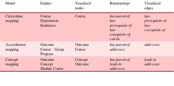
To visualize the curriculum network, we could simply draw all entities and relationships as nodes and edges, as many graph visualizations do. However, we find that for the purposes of curriculum design and institutional analysis, it is more useful to visualize courses grouped into their respective departments, because this visual arrangement reflects the organizational structure of the institution and it also reflects the familiar structure of online course listings. Therefore, in our visualization application, we draw nodes for only courses, and edges between nodes for only has-prerequisite-of and has-corequisite-of relationships. Nodes are visually grouped into clusters, driven by the existence of has-parent-of relationships. The types of entities and relationships for the curriculum network model and its visualization can be seen in Table 1.
Our educational network models are defined by different types of entities and relationships. Each model has a tailored visualization strategy
2.3 The accreditation mapping model
Accreditation mapping is the process of mapping learning evidence to accreditation outcomes in order to show how accreditation outcomes are met. As well as supporting program evaluation, accreditation mapping is used in curriculum redesign (Plaza et al. Reference Plaza, Draugalis, Slack, Skrepnek and Sauer2007; Kelley et al. Reference Kelley, Mcauley, Wallace and Frank2008).
We define an accreditation mapping network model as follows. We define four different types of entities: Outcome, Course, Group and Program. An ‘outcome’ here refers to an outcome used as a criterion in an accreditation study, such as the Accreditation Board for Engineering and Technology (ABET) student outcomes. These outcomes are typically defined by an external accreditation agency. A ‘group’ here refers to a way in which courses might be grouped (for example, as ‘required courses’, or ‘elective courses’, or ‘capstone courses’, etc.). A ‘program’ refers to a program of study, typically a degree program. We then define all the individual entities in the accreditation mapping network model: we define the individual outcomes, the individual courses, the groups, and the program. Each one of these entities is modeled as a vertex in the accreditation network model.
We define two types of relationships: has-parent-of and addresses. As in the curriculum model, the has-parent-of relationship is a directed relationship that specifies organizational hierarchy; in this case it relates courses to a group, and groups to a program. The addresses relationship is a directed relationship that indicates that a course addresses an outcome. These relationships are modeled as directed edges between the appropriate vertices in the accreditation network model. We create a directed edge of has-parent-of type from Course A to Group X if Course A belongs to Group X (examples of groups are Elective Courses, Core Courses, Capstone Courses, etc.). Similarly, we create a directed edge of addresses type from Course A to Outcome T if Course A addresses Outcome T. The addresses edges are assigned a weighting to indicate how strongly a course addresses an outcome. Figure 5 shows this accreditation mapping model ontology. Note that one could easily introduce additional types of entities and/or relationships to the model as desired.
The accreditation mapping model ontology. Left: the general ontology. Right: a concrete example.

With the accreditation network model defined, graph analytics reveal how program structure relates to accreditation requirements. The indegree of an outcome vertex defines how many courses contribute to addressing that outcome. For a given course vertex, the outdegree corresponding to edges of type addresses defines the number of outcomes addressed by that course. Analyzing the distribution of indegree and outdegree over the network model gives insight into a program’s strength of coverage across outcomes.
As with the curriculum model, a tailored graph visualization is more useful than a generic graph visualization. In our visualization application, we draw nodes for only courses and outcomes. We visualize courses grouped into their respective groups and programs, driven by the existence of has-parent-of relationships. We draw edges between nodes for only addresses relationships. The types of entities and relationships for the accreditation network model can be seen in Table 1.
2.4 The concept mapping model
In our concept mapping network model, we define four different types of entities: Outcome, Concept, Module and Course. In our ontology, a ‘module’ is a unit of curricular organization smaller than a course. The size of a module may vary, but we find that a typical semester-long course tends to comprise three to six modules. An ‘outcome’ here may refer to an accreditation outcome as in the accreditation mapping network model, but more often it refers to a learning outcome. Such learning outcomes are sometimes prescribed by an educational institution or governing body (for example, as is the case in some community college systems), or they may be authored by individual course instructors. We use the term ‘concept’ to denote the main idea underlying a (typically small) unit of content covered in the course. In our terminology, a concept is one example of a so-called ‘Knowledge Component’, as described in the Knowledge-Learning-Instruction framework in Koedinger et al. (Reference Koedinger, Corbett and Perfetti2012).
We define three types of relationships: has-parent-of relationships, addresses relationships, and leads-to relationships. The has-parent-of relationship is a directed relationship that specifies organizational hierarchy; in this case it relates outcomes to modules, concepts to modules, and modules to courses. The addresses relationship is a directed relationship indicating that a concept addresses an outcome and may be weighted to indicate strength of connection. The leads-to relationship is a directed relationship between outcomes and is used to represent prerequisite relationships among outcomes as described in the outcomes mapping framework of Seering et al. (Reference Seering, Willcox and Huang2015). Thus, our concept map represents relationships between outcomes and concepts, as well as relationships among the outcomes themselves. Figure 6 shows this concept mapping model ontology.
Our visualization application for the concept map draws nodes for concepts and outcomes. Using the specified has-parent-of relationships, we visualize concepts and outcomes grouped into modules, and modules grouped into their respective courses. We draw a directed edge from a concept node to an outcome node to visualize an addresses relationship. We draw a directed edge from one outcome node to another outcome node to show a leads-to relationship. The types of entities and relationships for the concept map network model can be seen in Table 1.
A concept mapping model ontology. Left: the general ontology. Right: a concrete example.

3 Educational mapping
In this section we define and describe our process of mapping. Here, we define the mapping process as the process of transforming an initial data set into a mapped data set consisting of entities and relationships as described in our network models.
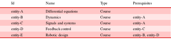
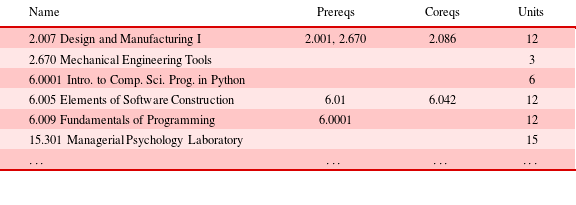
Table 2 shows a list of notional raw input data. The input data may come in many forms, but often its form will be similar to that depicted in Table 2. Mapping is the process of converting this data set into a structured form according to the mathematical network models presented in the previous section.
Before mapping: input data
The first step in mapping is to identify the entities of interest in the system. We step through the data set and construct entity objects. We assign each entity a unique identifier, and attach to it its type and other attributes. The constructed entity object may be minimally described in plain-text JavaScript Object Notation (JSON)Footnote 4 as:
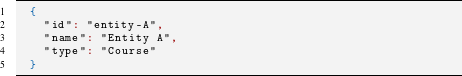
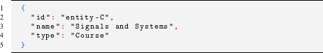
To illustrate with a concrete example, a JSON representation of the entity in the third row of Table 2 can be:
The second step in mapping is to construct relationship objects – we emphasize the construction of relationships as explicit objects. Current modeling formalisms flatten relationships to be attributes of an entity, as seen in Table 2. As discussed in Artale et al. (Reference Artale, Franconi, Guarino and Pazzi1999), such attribute-based modeling makes it difficult to analyze the ontological structure of the data and requires ad hoc mechanisms to derive inferences. For example, attribute-based modeling makes it difficult to ask questions about pathways such as, what courses are joined to other courses that are in themselves joined to other courses via prerequisites? The explicit modeling of relationships is a key contribution of our educational modeling work. Our graph model explicitly models relationships and entities, enabling reusable analyses at large scale.
We create an object for every relationship that appears, and assign the relationship a unique identifier. We also assign attributes representing the directionality, weighting, cost and other attributes of each relationship. For example, a relationship object such as the prerequisite requirement specified in the third row of Table 2 may be minimally represented in JSON as:
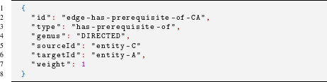
In this JSON example, the fields sourceId and targetId point to the unique identifiers of the source and target entity objects (here the Signals and Systems course with ID entity-C has a prerequisite of the Differential Equations course with ID entity-A). The field genus indicates whether the relationship is directed or undirected. Additional attributes may be present, depending on the data and application use case.
4 Results
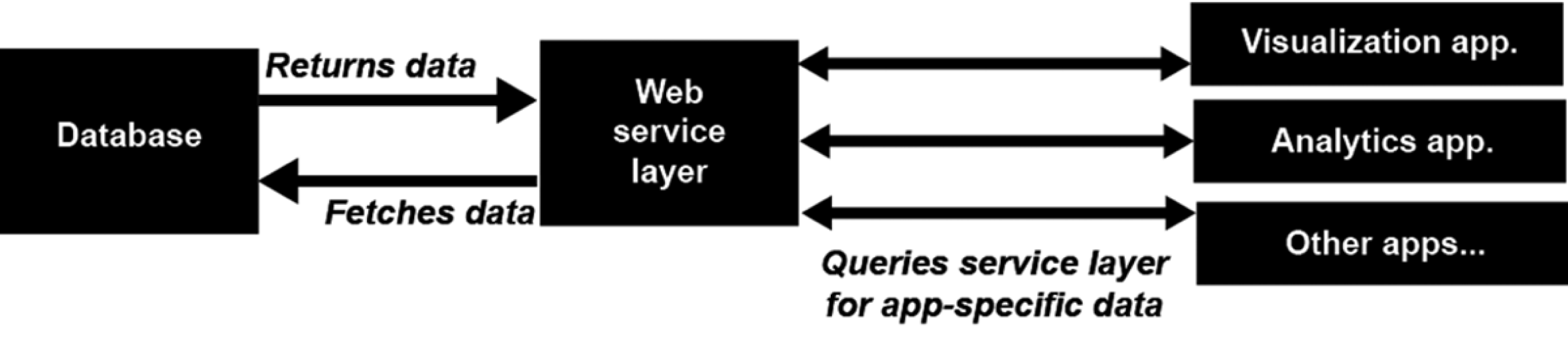
In this section we present three case studies to demonstrate application of our network-based educational models at multiple scales: (1) curriculum mapping at the institutional level, (2) outcomes-based accreditation at the degree program level and (3) instructional planning at the course level. In each case, we describe the mapping process and the resulting network model. We present example visualizations and analytics to illustrate the power of the modeling approach. Our implementation uses a scalable decoupled architecture that enables data to be accessed by multiple independent applications (in our case analytics and visualization) as illustrated in Figure 7.
A decoupled architecture consisting of three layers, from left to right: the backend, the web service, and the frontend applications.
4.1 Modeling at the institutional scale
In this example, we model the undergraduate curriculum of the Massachusetts Institute of Technology (MIT).
4.1.1 Mapping
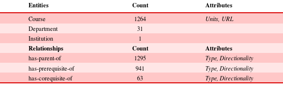
The MIT curriculum model uses the structure specified in Table 1. From a curriculum file provided by the MIT registrar office, we create the mapped data set consisting of entities and relationships as described by our network model. This data set represents a snapshot of the MIT undergraduate curriculum as of Fall 2015. Table 3 shows a sample of the input data file to the mapping process.
The first step in the mapping process is to identify the entities. To create the curriculum mapping, we step through each row of the input file and construct an entity of type Course for each row. We attach a units attribute for each course entity, which indicates the number of units (credits) associated with the course, and a URL attribute, which points to the course listing at the official MIT registrar website. We further construct entities of type Department for each unique department by parsing the number of the courseFootnote 5 . Finally we construct one entity of type Institution, representing the institution MIT.
The second step in the mapping process is to construct relationship objects. To do this, we make a second pass through the data and construct a relationship object for every prerequisite and corequisite requirement that appears in the entity’s Prereqs and Coreqs columns. We also construct a has-parent-of relationship object for every Course–Department relationship and every Department–Institution relationship. Table 4 summarizes the mapped data set.
Before mapping: sample of MIT curriculum file
After mapping: summary of mapped MIT curriculum data set
4.1.2 Analysis
Figure 8 shows a snapshot of the resulting network visualization, in which courses are visualized as nodes, clustered by their parent departments. The zoomed-in views illustrate the prerequisite relationships visualized as directed edges between the appropriate course nodes. In the example shown, we use node color to visualize how courses vary in unit count across the institute. A standard MIT course is 12 units (representing 12 total hours per week over a semester of length 14 calendar weeks). In Figure 8, orange nodes represent courses that are greater than 12 units – these are typically laboratory and project-based courses. As well as laboratory and project-based courses across the engineering and science departments, we see in Global Studies and Languages several courses that include research projects conducted in the relevant foreign language. Blue nodes represent courses that are fewer than 12 units. Here, we see evidence of the recent curricular redesigns of several MIT departments to include more flexibility in their undergraduate degree programs. For example, Mechanical Engineering at MIT offers a both a traditional and a flexible degree program. In the flexible degree program, students complete a core in mechanical engineering and combine it with a six-course concentration in one of several modern engineering areas. In part, this flexibility is enabled through half-semester courses (6 units) in the mechanical engineering core. The highlighted pathway in Figure 8 shows a full-semester course Mechanics and Materials I leading to a half-semester course Thermodynamics, which in turn leads to another half-semester course Introduction to Heat Transfer. Mechanics and Materials I is required for students in both the traditional and the flexible mechanical engineering degree programs. The two follow-on six-unit courses are required for the flexible degree program (whereas the traditional degree program has a different requirement), but the offering as two half-semester courses is intended to give the students greater scheduling flexibility to accommodate their broader degree requirements.
Visualization of MIT curriculum mapping: gray nodes indicate courses with 12 units (a standard semester-long course), blue nodes indicate courses with fewer than 12 units, and orange nodes indicate courses with more than 12 units. Here, three zoom levels of the visualization are shown.

Another analysis of the curriculum model is of prerequisite relationships. For each course, we find its entire prerequisite chain – i.e., the course’s prerequisites, the prerequisites of its prerequisites, and so on. This prerequisite chain is a subgraph within our network model. We then compute a topological sort on the subgraph to find a valid ordering of the prerequisite pathway of the course. Figure 9 visualizes some prerequisite pathways in a tree-like structure. In the visualization, nodes are ranked according to the maximum length of the pathway from the source node(s) in the subgraph to that node. Shown is a collection of prerequisite pathways with courses ordered by increasing rank. Note that the maximum length of the pathway represents the most constraining set of prerequisite requirements that the student must complete before they can take that course. For example, in Figure 9(c), the course Intro to EECS I is shown in the third level of the tree-like structure, because students must complete two levels of prerequisite classes (here Physics II and its prerequisites) before taking Intro to EECS I. Similarly, the course Intro to Algorithms has a longest path that requires three levels of prerequisite courses. Note that in the interest of presenting a simple illustrative graphic, these visualizations do not attempt to represent ‘or’ conditions in the prerequisite pathways.
(a) The MIT course 2.00 Introduction to Design has a rank of 0. (b) The MIT course 18.03 Differential Equations has a rank of 2. (c) The MIT course 6.006 Introduction to Algorithms has a rank of 3. (d) The MIT course 6.814 Database Systems has a rank of 5. These panels visualize the prerequisite pathways of courses. Within a pathway, course nodes are ordered by increasing rank. In all cases the directionality of the edges between courses points downwards.

4.2 Modeling at the program scale
In this example, we model an individual program – the Engineering Product Development (EPD) degree program at the Singapore University of Technology and Design (SUTD). We discuss how our network model can be used to support accreditation analysis.
4.2.1 Mapping
The SUTD EPD program model uses the structure specified in Table 1. We obtained from SUTD a list of program learning outcomes and courses, organized into groups according to the type of course. In this case, the outcomes are specified by an external accreditation agency. Each course has a list of outcomes that it addresses. The degree to which a course addresses an outcome is indicated by a numeric weighting from one (addresses weakly) to three (addresses strongly). This list and the weights were created by the SUTD faculty and curriculum coordinators. To create the accreditation mapping network model, we step through the list to construct entity objects for each outcome, course, grouping and degree program that appear. These constructed entities are vertices in the network model and have type of Outcome, Course, Group or Program. We also attach attributes to each entity, such as an URL for each course that directs the user to a repository of materials for that course, including evidence that is provided to accreditors during a site visit.
The second step in the mapping process is to construct relationship objects. To do this, we make a second pass through the list and construct a relationship object of type addresses pointing from each course to the corresponding outcomes. These relationships are each assigned a weighting. We construct a has-parent-of relationship object for every Course–Group, Outcome–Group, and Group–Program relationship.
After mapping: summary of the mapped SUTD EPD data set
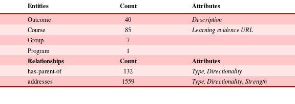
Table 5 summarizes the mapped data set and Figure 10 shows a snapshot of the resulting network visualization. In our visualization application, we visualize outcomes as nodes (small red circles) and courses as nodes (larger circles). The color of a course node indicates the number of outcomes it addresses, with whiter nodes addressing more outcomes and darker nodes addressing fewer outcomes. Groups are used to visually cluster outcomes and courses using has-parent-of relationships and for suburb labels in the map. The addresses relationships are shown as arrows pointing from a course node to an outcome node.
Visualization of SUTD Engineering Product Development degree program mapping. Outcome nodes are shown as small red circles and course nodes are shown as larger circles. Whiter course nodes address more outcomes and darker course nodes address fewer outcomes. The mouseover on the right shows which courses address the highlighted outcome.

4.2.2 Analysis
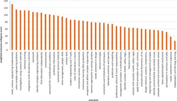
This network model provides a basis on which to conduct analysis of the program and its coverage of accreditation outcomes. For each outcome we can analyze its coverage in the EPD program. The indegree of an outcome vertex specifies the number of courses that address that outcome. The weighted indegree of an outcome vertex is computed by summing up the weights of the incoming edges. This gives an indication of the strength of coverage of that outcome across the curriculum. For example, the outcome ‘Identify responsibilities relevant to professional engineering practice through a clear needs statement in capstone or design projects’ is addressed by the following courses (weighting shown in parentheses): Introduction to Design (1), Modeling the Systems World (1), The Digital World (1), Engineering Design & Project Engineering (2), Capstone (3), Entrepreneurship (3), Power Electronics (1), Design & Fabrication of MEMS (1), Electric Power Systems Analysis and Design (1), Micro-Nano Projects Laboratory (2), Digital Integrated Circuits Design (1), Topics in Biomedical & Healthcare Engineering (1), Design Management (3), Design and Manufacturing (1), Engineering Management (2), Culture Formation and Innovative Design (3), Energy Systems (3), Urban Transportation (1), The History of International Development in Asia: The Role of Engineers and Designers (1), Social Theories of Urban Life (1), Who Gets Ahead? Sociology of Social Networks and Social Capital (2), Rice Cultures: Technology, Society, and Environment in Asia (2), How the Things People Make, Make People: Material Things in Social Life (1). This gives a weighted indegree score for the outcome vertex of 38.
Figure 11 plots the weighted indegree scores for all 40 outcomes. These data emphasize the strongly interdisciplinary and design-focused nature of the SUTD curriculum, with a strong mapping between courses and outcomes. This strong mapping is not coincidental – SUTD is a newly founded university and its curriculum was designed from scratch to emphasize cross-cutting skills and challenges, rather than the traditional disciplinary approach of most engineering programs. In general, this kind of network analysis will reveal potential gaps of coverage in a curriculum, although in the SUTD EPD case, no such gaps are apparent.
The weighted indegree score for each outcome shows how strongly the outcome is addressed by courses across the SUTD EPD curriculum.
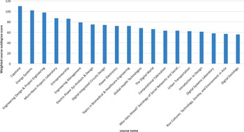
An analysis of course vertices reveals how strongly a particular course contributes to addressing program outcomes. Similar to the weighted indegree calculation described above, we can compute the weighted outdegree of a course vertex by summing the weights associated with all outgoing addresses relationship edges. Figure 12 plots the results for the 20 courses in the SUTD EPD curriculum that have the highest outdegree scores. These analytics are useful, for example, in considering the effects of curriculum redesign on coverage of program outcomes. These scores could also be combined with student enrollment data to provide a quantitative assessment of student coverage of outcomes, either by individual student or in aggregate across the student population.
The weighted outdegree score for each course shows how strongly the course contributes to outcomes across the SUTD EPD curriculum.
To further illustrate the utility of this analysis, we create a notional student plan of studyFootnote 6 , which identifies the courses taken or planned to be taken by a particular (notional) student who we term ‘Student X’. We layer Student X’s data on the accreditation network model, in order to analyze the strength of outcome coverage specifically for Student X, projected upon completion of their degree program. Figure 13 shows for this notional example the projected distribution of coverage for Student X. The red bars in Figure 13 highlight two outcomes that have low coverage scores: (1) recognize the need for and prepare for independent and life-long learning and (2) regular participation in seminars and talks. To remedy the deficiency in these two outcomes, the student would be advised to take a course that addresses these outcomes. With the network model in hand, we can immediately generate a recommendation for a course that strongly addresses both of these outcomes. Figure 14 shows a companion visualization that highlights this recommendation. In this case, the course Sociology of Social Networks and Social Capital is identified to be a course with one of the highest addresses edge values.
The projected outcome coverage of Student X, shown in increasing score. A red bar indicates that Student X has a potential deficiency for that outcome with the current plan of study.

The projected outcome coverage of Student X was found to be deficient in two outcomes, highlighted in red. To alleviate this deficiency, the highlighted blue course that addresses both outcomes is recommended to the student in an advising session.

4.3 Modeling at the course scale
In this example we model and map a single course, Computational Methods in Aerospace Engineering.
4.3.1 Mapping
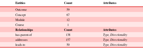
The concept map model uses the structure specified in Table 1. The course has 59 learning outcomes describing what a student is expected to be able to do after completing the course. The instructor identified 67 concepts, highlighting what she thought to be the key topics covered in the course. These outcomes and concepts are grouped into four modules: integration methods for ordinary differential equations (ODEs), finite difference and finite volume methods for partial differential equations (PDEs), finite element methods for PDEs, and probabilistic simulation and Intro to design optimization. Within each of these modules, the concepts and outcomes are each grouped into a sub-module. This leads to the concept map network model with a total of 139 entities as shown in Table 6.
The second step in the mapping process is to construct relationship objects. Relationships contained in the provided course data include the relationships between concepts and outcomes; these specify which outcomes each concept addresses. The data also contain information on the relationships among outcomes, by specifying for each outcome a list of its prerequisite outcomes (i.e., the other outcomes that must be mastered in order to achieve that particular outcome).
After mapping: summary of mapped dataset for course Computational Methods in Aerospace Engineering
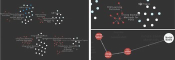
To construct the relationship objects in the network model, we step through each concept and identify the outcomes it addresses. For each, we construct a relationship object of type addresses pointing from the concept to the outcome. We step through each outcome and construct a relationship object of type leads-to pointing from the outcome to any downstream outcomes for which it is a prerequisite. We construct a has-parent-of relationship object for every Concept–Module, Outcome–Module, and Module–Course grouping. Table 6 summarizes the mapped dataset and Figure 15 shows a snapshot of the resulting network visualization.
Visualization of concept map for course Computational Methods for Aerospace Engineering.
4.3.2 Analysis
As with the accreditation map example above, an analysis of the indegree of outcomes and outdegree of concepts reveals how course content covers the course learning outcomes. One could further model the relationship between course assessments (exams, projects, homeworks, etc.) and outcomes. Layering student assessment results could then provide granular insight into student achievement of course learning outcomes.
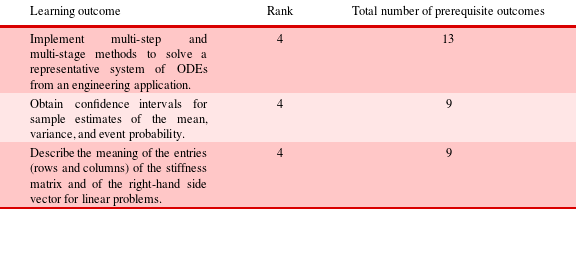
As one example of analysis on the concept mapping network model, we consider the subgraph corresponding to only the leads-to relationships and perform a topological sort of the subgraph. We then rank the outcomes according to the length of their prerequisite chains. The outcomes with the highest rankings are those that have the most prerequisites, and thus represent skills that build upon and synthesize upstream skills. In Computational Methods in Aerospace Engineering, the highest rank of an outcome is four. The three outcomes of rank four are shown in Table 7. This means that, for those three outcomes with rank four, there is at least one path that includes four prerequisite outcomes that lead to that outcome. Note that here it is the longest path that is of interest, because this represents the most constraining (in terms of number of prerequisite outcomes) requirement in the concept map pathways. The table also shows the total number of prerequisite outcomes for each outcome (including inherited prerequisites, i.e., prerequisites of prerequisites). For example, the outcome ‘Implement multi-step and multi-stage methods to solve a representative system of ODEs from an engineering application’ is a synthesizing outcome that requires students to have mastered upstream skills such as determining a method’s convergence properties, determining stability boundary, and explaining the difference between explicit and implicit methods. Figure 16 shows a tree visualization of this outcome and its prerequisite outcomes within the course. The rank of four is apparent from the number of levels in the tree-like structure. From the figure it can be seen that there are additional shorter pathways leading to this node (e.g., the pathway with just two prerequisite outcomes that flows through ‘Explain the Newton–Raphson method’); however, since a student must master all upstream outcomes, it is the longest pathway that is relevant in ranking the outcome.
Visualization of the tree-like structure yielded by the outcome Implement ODE integration methods and its prerequisite chain.
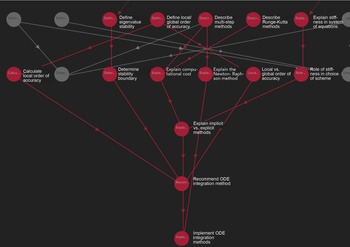
Outcomes of high rank are synthesizing skills that build on earlier material in the course Computational Methods in Aerospace Engineering
5 Conclusion
This paper has presented a flexible and scalable mathematical framework for educational modeling, with modeling examples ranging from an institutional-wide curriculum to an engineering degree program to a single course. The resulting network models embody the mappings that represent the rich relationships among different educational entities, such as courses, concepts, outcomes, departments and degree programs. The network models enable visualization and analytics, either using standard graph visualization and graph analytics tools, or using components tailored to the specific educational setting. In the examples presented, viewing the elements of an educational curriculum through the structured lens of a network model provides insight into learning pathways and permits gap analysis of curriculum coverage, supporting curricular design, student course planning and student advising.
It is important to note that in many cases the types of analyses presented in this paper depend critically on data provided by instructors and faculty. For example, in the accreditation mapping example, instructors provide the data that specifies which accreditation outcomes are addressed by their courses and to what extent (via the weightings). Similarly, in the concept mapping example, the instructor provided the learning outcomes and defined their relationships to the concepts. The conclusions drawn from the analysis methods presented in this paper will only be as good as the data on which they are built, although in this regard scalable visualization can be a valuable way of communicating and checking data.
For privacy reasons, this paper has avoided any examples that use actual student data; however, clearly the presented models provide a structured foundation that, in concert with student data, could enable data-driven advising, adaptive learning, personalized learning and data-driven institutional resource allocation.
Acknowledgments
The authors thank Ri Romano of MIT and Toe Oo Zaw of SUTD for their help in collecting the data used in the examples. This work was supported in part by the International Design Center as part of the MIT-SUTD Collaboration.


 Open access