

1 Motivation
The complexity of high-stakes engineering systems, such as airplanes and space systems, means that design engineers require scalable failure analysis techniques to ensure system safety. However, since sub-systems are often designed independently (i.e., by separate engineering groups or companies), sub-system interactions are not completely known even if specified through interface protocols until a prototype is built and tested. At the prototype building stage of the design process, changes are costly. To reduce cost, it is desirable to understand a system’s failure behavior early in the design process. However, early stage design presents a significant challenge for designers, including lack of detailed knowledge of the system hardware. Engineering design has recently turned to network analysis as a new technique for understanding the failure tolerance of complex engineered systems in the absence of fully built prototypes and simulations.
2 Aim and significance
Prior research introduced the idea of using a behavioral network and network metrics to understand the failure tolerance of complex engineered systems (Haley et al. Reference Haley, Dong and Tumer2014, Reference Haley, Dong and Tumer2016). Behavioral networks represent complex engineered systems with a network-based representation in which nodes represent design variables and parameters and edges represent relations between them. We call these nodes parameter nodes. The relations (edges) between nodes are derived from behavioral descriptions of complex engineered systems, which include but are not limited to governing equations and model-based design representations. This prior work developed the method known as behavioral network analysis (BNA). BNA introduced a method to relate the local failure of nodes in behavioral networks to system-level failures through the use of specific microscale, i.e., local, node-level, network metrics. BNA showed the novel result that local perturbations to behavioral network-based representations of complex engineered systems can reveal system-level behavioral faults. An important limitation of the prior research was that BNA cannot identify a priori which nodes, when in a fault state, are most likely to be associated with significant degradations of system-level performance. Building on this method, this article aims to show that bridging nodes, which are nodes that connect communities, or modules, in the behavioral network are associated with a large change in a topological network metric average shortest path length (ASPL) when under attack. An attack simulates the failure of nodes or edges on system-level behavior. What this means is that the behavioral degradation of a system is intrinsically linked to the community structure of its behavioral network. To show this, the hypothesis to be tested is that the behavioral degradation of complex engineered systems is higher when bridging nodes are subject to attack than when non-bridging nodes are subject to attack, as measured by the network metric ASPL.
An experimental study with forty engineering systems is used to test this hypothesis. The experiment tests the change in the ASPL when bridging and non-bridging nodes are attacked, that is, removed from the behavioral network representation. During the attack, the edge weights of edges associated with a node are modified. The fault variable is a factor that describes the degree of degradation of a node (Haley et al. Reference Haley, Dong and Tumer2014, Reference Haley, Dong and Tumer2016). Performing the test under a range of values for the fault variable tests the sensitivity of the BNA method on the value of the fault variable.
In addition to testing this hypothesis, this article extends BNA modeling techniques (Haley et al. Reference Haley, Dong and Tumer2014, Reference Haley, Dong and Tumer2016). The article introduces new techniques to model embedded behaviors, represented by function calls, and logical behavior, described by discrete equations.
3 Outline
First, a conceptual proof is presented to demonstrate how ASPL relates to bridging nodes. Then, the forty systems used to test the hypothesis are described in terms of size, type, and other characteristics. Next, modeling advances necessary to build behavioral networks for these systems are presented. The hypothesis tested is whether bridging nodes under attack are associated with a larger change in ASPL than non-bridging nodes in the network. The experimental study uses a t-test to show whether or not there is a statistically significant difference between the change in ASPL between bridging and non-bridging nodes from nominal to fault cases. The latter part of the article explores the effect of the fault variable on the ASPL method. The article ends with a general discussion of the findings and a section on future work.
4 Background
4.1 Existing failure analysis methods
Many methods for failure analysis take place late in the design process. Designers often use Failure Modes and Effects Analysis (FMEA) to decompose a system into sub-systems and components to explore possible failure modes and their effects on the system (Department of Defense 1980). The downside of FMEA is that it relies on engineering expertise, knowledge of the system, and historical data. This limits its usefulness for novel designs. Another widely used method, Fault Tree Analysis (FTA), shows paths leading to undesirable system states (Vesely et al. Reference Vesely, Goldberg, Roberts and Haasi1981). The usefulness of FTA, however, depends on the accuracy of the system representation, which can be lacking in the early design stages. Another design method is the use of a Reliability Block Diagram (RBD) (Jensen Reference Jensen2012). An RBD represents system architecture and component relationships graphically using failure rate information. If information is required for systems with dynamic behavior, it may be necessary to use a more advanced technique such as Markov analysis (Xue and Yang Reference Xue and Yang1995). A problem with such techniques is that they require accurate failure probabilities and independent failures (Jensen Reference Jensen2012). These may not always be the case in real-world complex engineered systems. These methods are therefore limited by the accuracy of the failure probabilities, independence of failures, and lack of usefulness early in the design process.
More recently, efforts have been made to move failure analysis to early stage design. This includes methods such as the Function-Failure Design Method (FFDM) (Stone et al. Reference Stone, Tumer and Van Wie2005). An extension of FFDM, Risk in Early Design (RED), takes into account likelihood estimates (Grantham Lough et al. Reference Grantham Lough, Stone and Tumer2007, Reference Grantham Lough, Stone and Tumer2008). FFDM and RED connect system failures to loss of function in order to identify potential failures. It then considers historical data so it can predict which failure modes are likely. It is therefore reliant on the availability of such data. Another method available in the conceptual design stage is Functional Failure Identification and Propagation (FFIP) (Kurtoglu et al. Reference Kurtoglu and Tumer2008). FFIP provides designers with information on failure behavior considering component, function, and behavior implementations. However, FFIP uses a behavioral simulation to determine fault propagation paths, which is computationally costly.
Taking an alternative approach, BNA makes the assumption that complex engineered systems can be represented by behavioral networks that abstract behavioral relations from a system and then represent those relations as a network. This network is the basis for the analysis of the tolerance of the complex engineered system to systemic failure.
4.2 Network analysis in engineering design
The fundamental idea behind BNA is that complex engineered systems can be represented as a complex network, a modeling formalism that has led to significant insights in multiple fields including social networks (Pattison et al. Reference Pattison, Wasserman, Robins and Kanfer2000), the world wide web (Albert et al. Reference Albert, Jeong and Barabási1999), and biology (Jeong et al. Reference Jeong, Tombor, Albert, Oltvai and Barabási2000; Sole et al. Reference Sole, Ferrer-Cancho, Montoya and Valverde2003). Complex network theory has already been applied to engineering design in a number of ways. A network approach has been used to analyze system modularity (Sosa et al. Reference Sosa, Eppinger and Rowles2007), analyze the effect of design changes (Ma et al. Reference Ma, Jiang and Liu2016), and predict customer responses to technological changes (Wang et al. Reference Wang, Sha, Huang, Contractor, Fu and Chen2016). Recent research has uncovered that the network structure of products and product development processes resembles many other real-world networks (Braha and Bar-Yam Reference Braha and Bar-Yam2004).
The idea behind using network analysis to understand system failures is to find an appropriate way to represent a complex engineered system as a complex network and use various techniques from network theory for analysis (Sosa et al. Reference Sosa, Mihm and Browning2011; Sarkar et al. Reference Sarkar, Dong, Henderson and Robinson2014). This is possible because of meaningful analogies between complex networks and complex systems (Mitchell Reference Mitchell2006), specifically with regard to failure behavior. The complex network perspective explicitly considers the relation between structure and function, that is, how entities come together in order to perform a function (intended purpose). It also explicitly considers the relation between structure and systemic risk of connectivity failure based on the interdependence of nodes. Simply put, the structure of the network affects how effectively a system accomplishes its functions and its resistance to systemic failure.
Much as a contagion spreads in a biological system, a failure in an engineered system can cause loss of performance downstream (Mehyrpouyan et al. Reference Mehrpouyan, Haley, Dong, Tumer and Hoyle2013a ). Failure in a complex network is described as fragmentation of the network into smaller, disconnected parts and is generally measured using size-based metrics such as the diameter of the network or the size of the largest connected component of the network. It is assumed that in the network’s original state, every node is connected to at least one other node in the network. An attack on a network can be either random or targeted, meaning nodes and edges are attacked (removed from the network) at random or due to specific properties such as their high degree of connectivity. A network’s ability to withstand attack has been well researched in other fields (Albert et al. Reference Albert, Jeong and Barabási2000; Sosa et al. Reference Sosa, Mihm and Browning2011). For instance, scale-free networks are vulnerable to targeted attacks on nodes having a high degree of connectivity but robust to random attacks (Albert et al. Reference Albert, Jeong and Barabási2000). In an engineering system, a random node attack is similar to a random failure whereas a targeted attack is similar to a failure initiated by a known external event that will impinge directly on the target node (design variable or parameter). For example, rain and fog can interfere with specific components in radar-based detection systems, compromising the system’s performance. For this reason, the transfer of knowledge about the failure of complex networks and complex engineered systems is possible.
4.3 Behavioral modeling
To understand how vulnerable a system is to the loss of function in an individual element in the system, previous work developed the concepts and mathematics behind network representations of engineering systems (Kasthurirathna et al. Reference Kasthurirathna, Dong, Piraveenan and Tumer2013; Mehyrpouyan et al. Reference Mehrpouyan, Haley, Dong, Tumer and Hoyle2013a ; Mehrpouyan et al. Reference Mehrpouyan, Haley, Dong, Tumer and Hoyle2013b ). The predominant modeling approach has thus far been to represent the components and their inter-relationships in the system as a network. The problem with using only the components in the network model is that the network model insufficiently represents behavioral interactions. Depending upon the assumptions used to create the component-based model, interactions between components may include physical connections or spatial interactions, such as a magnetic flux from one component that may impact nearby components. Any behavioral interaction is implied in the component model and it is not evident which interactions have been included and which have been excluded. In complex engineered systems, multiple design variables and parameters are often shared among components and sub-systems. Component models do not necessarily model the interaction between components due to these shared parameters. Taking into account behaviors rather than physical architecture alone means that a broader range of failure possibilities and sub-system interactions can be considered (Haley et al. Reference Haley, Dong and Tumer2014, Reference Haley, Dong and Tumer2016). Furthermore, while other methods of failure analysis rely on expert knowledge such as failure probabilities, failure behavior known through experience, and specific component selection, BNA does not. The advantage of BNA lies in early stage design, especially of novel systems, when this information is not known.
5 Related work
5.1 Prior work in behavioral network analysis
5.1.1 BNA overview
Given the lack of work on network-based behavioral representations, initial research in BNA focused on the details of modeling a complex engineered system. BNA utilizes a behavioral model rather than a component-based model or a typical functional model. One of the assumptions of BNA is that the mathematical details of the governing equations of the system can be abstracted into a network representation. Subsequent experimental results indicate that the network representation is sufficient to obtain valuable information about the failure tolerance of the system. Abstracting away the mathematical details, and instead focusing on the structural role of the parameters in a behavioral network representation, saves a significant amount of computational cost. BNA is not expected to provide quantitative predictions regarding the effect of the degradation of a particular parameter, that is, to provide the exact values of parameters and variables at the time of a particular failure. Instead, the concept of the local degradation of a parameter causing global system-level impact, and its analogy to what happens in a complex network when a node is removed, is at the core of BNA.
Given the network representation, BNA uses network topology metrics to find vulnerable parameter nodes in the behavioral network (Haley et al. Reference Haley, Dong and Tumer2014, Reference Haley, Dong and Tumer2016). The degradation of parameter nodes should cause a system-level change. In order to test which network topology metrics could detect system-level changes due to attacks on nodes in the behavioral network, prior work compared multiple network metrics (Haley et al. Reference Haley, Dong and Tumer2014, Reference Haley, Dong and Tumer2016) based on their ability to indicate the system-level effects of node attack. Attacking a node in BNA involves decreasing the edge weight of all edges associated with the target (attacked) node from 1.0 to 0.5. In other words, a fault variable of 0.5 is applied to that parameter. Complete node removal would involve applying a fault variable of zero to all edges associated with the target node. However, using a fault variable value greater than zero (but less than one) is more representative of what happens in the engineering system, which is that a parameter’s value is different from its nominal value but some functionality is retained. It was found that two network metrics, ASPL and robustness coefficient (Piraveenan et al. Reference Piraveenan, Thedchanamoorthy, Uddin and Chung2013), sufficiently captured the behavioral degradation due to attack on parameter nodes (Haley et al. Reference Haley, Dong and Tumer2014, Reference Haley, Dong and Tumer2016). This prior research showed that behavioral networks of complex engineered systems can be used to detect system-level faults due to local failures. However, the method could not determine in advance which nodes would most likely be associated with system-level faults. In other words, if a system-level fault is detected, which nodes may be the cause? Or, alternatively, if certain nodes fail, which ones are most likely to cause the most significant changes to the system?
Previous work by the authors (Walsh et al. Reference Walsh, Dong and Tumer2017) introduced the concept of bridging nodes to understand the structural role of vulnerable parameters in behavioral networks of complex engineered systems. In this article, the authors delve deeper into this idea. The new contributions of this article are a conceptual proof for a higher change in ASPL for bridging nodes than non-bridging nodes, a study on the effect of the value of the fault variable on system-level failure, additional empirical results on the degree distributions of real-world behavioral networks, and findings on the relationship between the community structure of behavioral networks and their failure tolerance.
5.1.2 BNA system representation
The technique outlined in this section is based on the work by Haley et al. (Reference Haley, Dong and Tumer2014, Reference Haley, Dong and Tumer2016). The first step in BNA is to build the behavioral network from the system’s set of governing equations. Each individual function in the set of governing equations is referred to by a numbered function, for instance $F1$
. The network is bipartite which means it has two distinct types of nodes. In bipartite behavioral networks, these two nodes types are function nodes and parameter nodes. Any given node in a bipartite network can share an edge only with a node of the opposite type. A bipartite network can be transformed into a unipartite network through an appropriate transformation.
$F1$
. The network is bipartite which means it has two distinct types of nodes. In bipartite behavioral networks, these two nodes types are function nodes and parameter nodes. Any given node in a bipartite network can share an edge only with a node of the opposite type. A bipartite network can be transformed into a unipartite network through an appropriate transformation.
Next, a group of nodes is assigned to describe each function. In practice, the set of functions describing the behavioral network can be extracted from any mathematical or behavioral description of the system. In this project, the systems are derived from system models in OpenModelica, version 3.2.2 (OpenModelica 2016) and the sets of functions are extracted from the instantiation information. Two functions from an example model from the standard OpenModelica package, a rolling wheel, are shown below. They are called $F1$
(the first function in the set of governing equations of the system) and
$F1$
(the first function in the set of governing equations of the system) and $F2$
(the second function in the set of governing equations of the system). A high-level description of this model is given in Appendix A. For each given function, such as the ones given below, there is one function node and at least one parameter node.
$F2$
(the second function in the set of governing equations of the system). A high-level description of this model is given in Appendix A. For each given function, such as the ones given below, there is one function node and at least one parameter node.
 $$\begin{eqnarray}\displaystyle & & \displaystyle F1:~\mathit{inertia.J}\times \mathit{inertia.a}=\mathit{inertia.flange}\_a.\mathit{tau}\nonumber\\ \displaystyle & & \displaystyle \quad +\,\mathit{inertia.flange}\_b.\mathit{tau};\end{eqnarray}$$
 $$\begin{eqnarray}\displaystyle & & \displaystyle F2:~\mathit{inertia.flange}\_a.\mathit{tau}+\mathit{torqueStep.flange.tau}=0.0;\end{eqnarray}$$
There are four parameter nodes in (1), one for each of the variables in the function. These are connected to the function node corresponding to the first function in the set of governing equations, $F1$
. The function node is
$F1$
. The function node is $F2$
for (2). There are two parameter nodes corresponding to its two variables. This process, done for all functions, forms the system’s behavioral network. See Figure 1 for the behavioral network in which nodes are ovals and edges are lines drawn between nodes.
$F2$
for (2). There are two parameter nodes corresponding to its two variables. This process, done for all functions, forms the system’s behavioral network. See Figure 1 for the behavioral network in which nodes are ovals and edges are lines drawn between nodes.
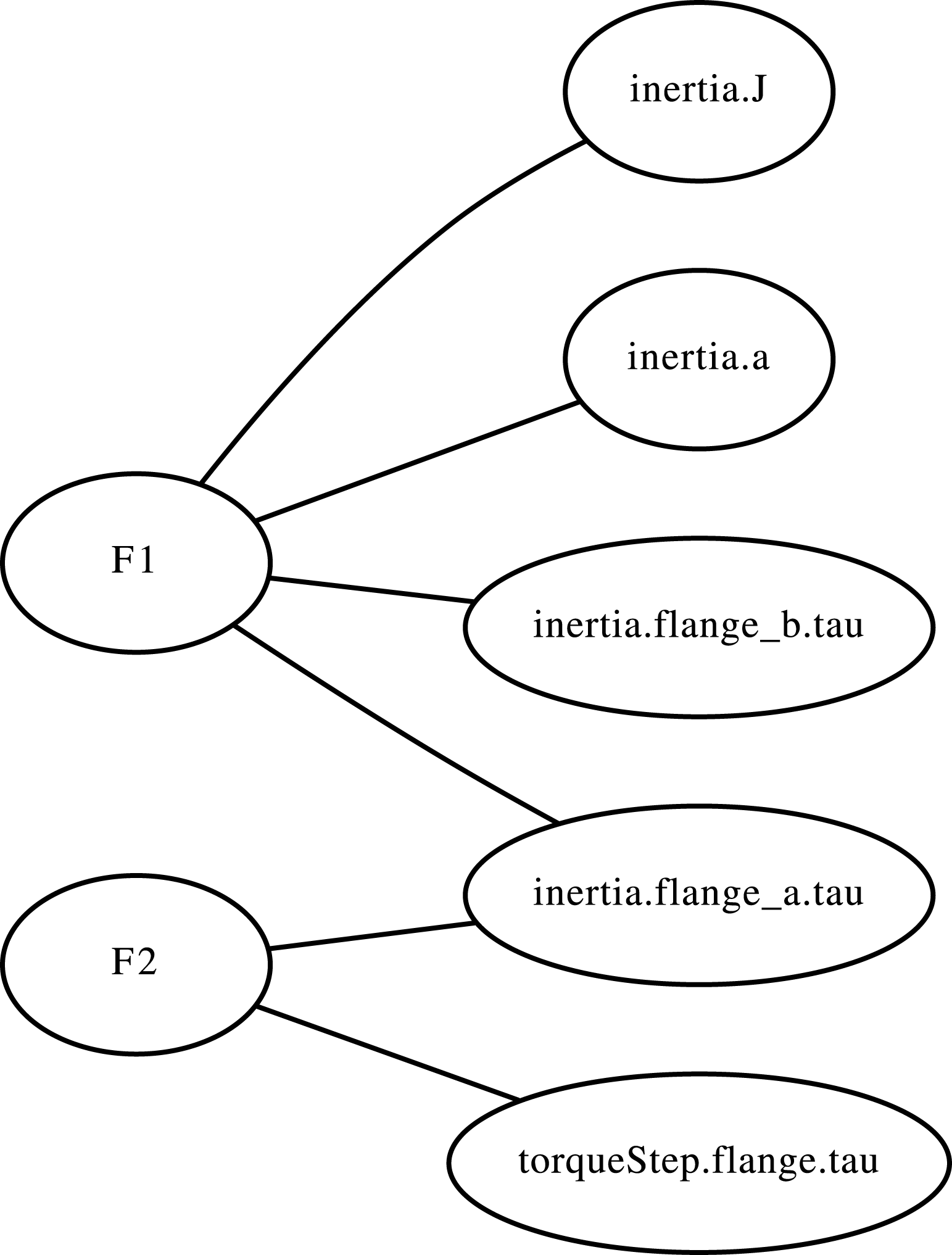
It is worth noting that for this example we have chosen two functions that share a design parameter. Not all functions in the set of governing equations will share a parameter. However, when the full graph is generated, all functions will be connected via at least one parameter node. Two given functions may not be connected together directly, but they will be connected together indirectly via other functions.
5.1.3 Finding vulnerable design parameters using BNA
At this point, the behavioral network has been constructed. The next step in the process is to calculate the network metric for the degradation of each parameter node. Parameter degradation refers to a change from its nominal value. In network analysis, failure is simulated by ‘attacking’ a node or edge, generally by removing a node and its associated edges or removing or changing the weight of an edge. In BNA, the parameter nodes are attacked by modifying the edge weights of associated edges. The reason for attacking parameter nodes and not function nodes is that, to the physical system, attacking a function node is meaningless. It is meaningful to attack parameter nodes because they correspond to real design parameters that may have out-of-nominal value depending on operating conditions, manufacturing tolerances, or failure. The value of the edge weight is used as an indicator of the degree of fault in the relation between nodes. Its value is known as the fault variable in the behavioral network. The general prescription is to modify the edge weights to 0.5, but this study will examine the effect of various values of edge weight. The network metric ASPL is calculated first for the nominal case and then for the case of degradation of each parameter. The first of these cases implies no fault. The second implies a fault. The ASPL is the average value of the shortest paths between all nodes in the network. ASPL has already been tested for its ability to capture behavioral degradation (Haley et al. Reference Haley, Dong and Tumer2014, Reference Haley, Dong and Tumer2016).
In the work by Haley et al. (Reference Haley, Dong and Tumer2014, Reference Haley, Dong and Tumer2016), the ASPL under an attack state is compared to the nominal ASPL, that is, the ASPL of the behavioral network in its original state. In this article, the difference between the nominal ASPL and a given degradation case ASPL was calculated and the resulting quantity is called the $\unicode[STIX]{x0394}\text{ASPL}$
of that parameter node. A large
$\unicode[STIX]{x0394}\text{ASPL}$
of that parameter node. A large $\unicode[STIX]{x0394}\text{ASPL}$
of a parameter node compared to other parameter nodes in the same system is expected to predict that this parameter (node) is vulnerable.
$\unicode[STIX]{x0394}\text{ASPL}$
of a parameter node compared to other parameter nodes in the same system is expected to predict that this parameter (node) is vulnerable. $\unicode[STIX]{x0394}\text{ASPL}$
is a measure of relative vulnerability. Vulnerable parameter nodes have with high
$\unicode[STIX]{x0394}\text{ASPL}$
is a measure of relative vulnerability. Vulnerable parameter nodes have with high $\unicode[STIX]{x0394}\text{ASPL}$
relative to other parameter nodes in the network.
$\unicode[STIX]{x0394}\text{ASPL}$
relative to other parameter nodes in the network.
5.2 Bridging nodes
Since the focus of BNA is on finding vulnerabilities, and because of the analogy between complex engineered systems and complex networks, vulnerabilities in networks are relevant. Finding vulnerable nodes in a network is a key area of research in network science (Li et al. Reference Li, Li, Jia, Liu and Yang2013). Vulnerable nodes in a network are typically described as those for which the removal would disconnect a large group of nodes from the main portion of the network or greatly increase the path length between nodes. Recently, some researchers have focused on locating bridging nodes, which are nodes that connect communities (Zhu et al. Reference Zhu, Wang, Di and Fan2014; Liu et al. Reference Liu, Xiong, Shi, Shi and Wang2016). While there is some debate on the exact mathematical definition of a community in a network, the generally accepted definition of a community is tightly connected groups of nodes that have more connections to nodes within the community than to nodes outside of the community (Newman Reference Newman2010). Bridging nodes have been shown to be relatively more vulnerable than other types of nodes in the network (Hwang et al. Reference Hwang, Cho, Zhang and Remanathan2006).
Communities are located in a particular network using a community detection algorithm. There are many methods for community detection, but this paper will focus on methods based upon the concept of modularity maximization. Modularity maximization begins with an initial division of nodes into communities, which is often a random division into equally sized communities. Then, the change in modularity metric is calculated in the case that each node individually were to move to the other community. Those nodes for which their movement would increase the modularity metric by the largest amount (or those for which their movement would decrease the modularity metric by the smallest amount) and which have not already been moved are then moved to the other community. Once all the nodes have been moved, the algorithm saves this state and begins the process again. When the modularity metric no longer improves at the end of the process, the algorithm terminates (Newman Reference Newman2010).

Figure 2. Heat transfer of two masses behavioral network, unmodified.
The Q-modularity of a community or group in the network is calculated using the relation in (3), where $m$
is the number of edges,
$m$
is the number of edges, $A_{ij}$
is an element of the adjacency matrix,
$A_{ij}$
is an element of the adjacency matrix, $k_{i}$
is the degree of vertex
$k_{i}$
is the degree of vertex $i$
,
$i$
, $\unicode[STIX]{x1D6FF}(m,n)$
is the Kronecker delta, and
$\unicode[STIX]{x1D6FF}(m,n)$
is the Kronecker delta, and $c_{i}$
is the community in which node
$c_{i}$
is the community in which node $i$
belongs. The Q-modularity is always less than 1. A positive modularity indicates that there is more interconnectedness within a community than would occur by chance alone, whereas a negative modularity indicates that there is less interconnectedness within a community than would occur by chance alone (Newman Reference Newman2010).
$i$
belongs. The Q-modularity is always less than 1. A positive modularity indicates that there is more interconnectedness within a community than would occur by chance alone, whereas a negative modularity indicates that there is less interconnectedness within a community than would occur by chance alone (Newman Reference Newman2010).
 $$\begin{eqnarray}Q=\frac{1}{2m}\mathop{\sum }_{ij}\left(A_{ij}-\frac{k_{i}k_{j}}{2m}\right)\unicode[STIX]{x1D6FF}(c_{i},c_{j}).\end{eqnarray}$$
Bridging nodes are nodes that have at least one connection from a node within a community to a node in another community. In a community, there are many nodes that have connections internal to the community and few nodes that have connections outside of the community. The latter type of node is a bridging node. Bridging nodes essentially connect communities. The definition of bridging nodes, then, is inseparable from the definition of communities.
The conjecture presented in this article is that bridging nodes have a significant role in the failure tolerance of behavioral networks. This is an interesting research question because it suggests a link between the community structure of behavioral networks and their failure tolerance. Communities of nodes exist in almost all networks, and they do not exist by chance. Whether by self-organization or intent, elements form communities to perform a higher-level function. From a physical architecture perspective, these communities represent sub-systems that perform a specific function. In behavioral networks, these communities are a collection of design parameters which perform a behavior. Though it would be highly unlikely that communities would not exist in behavioral networks, communities are not completely evident in the set of governing equations. Other than communities that are defined by a single equation, ‘emergent’ communities arise from the structure of the set of equations describing the systems. Figure 2 shows the behavioral network of an engineering system. Figure 3 shows the same behavioral network with the communities circled for purposes of illustration. This behavioral network is for the heat transfer of two masses system, described at a high level in Appendix A. These communities were located using a modularity maximization community detection algorithm. If a bridging node were to fail, then these behavioral communities would become disconnected from other behavioral communities in the system. This could cause a potential fault. Given the established relation between the change in ASPL and system-level failure, this article tests whether or not the change in the ASPL of bridging nodes is higher than the change in the ASPL of non-bridging nodes.

Figure 3. Heat transfer of two masses behavioral network, communities circled.
6 Research method
6.1 Conceptual proof
Considering the definition of ASPL and the definition of a bridging node, it can be shown conceptually that an attack on a bridging node induces a larger change in ASPL than an attack on a non-bridging node. The ASPL formula, given in (4) (Newman Reference Newman2010), considers the shortest path between all pairs of nodes in the network. In (4), $n$
is the number of nodes in the network and
$n$
is the number of nodes in the network and $d$
is the shortest distance between two nodes. The indices
$d$
is the shortest distance between two nodes. The indices $i$
and
$i$
and $j$
refer to individual nodes. The equation for ASPL indicates that a shorter distance between nodes decreases the ASPL. A visualization of this concept is shown in Figures 4 and 5. In Figure 4, a completely connected graph, each node neighbors every other node in the network. In contrast, in Figure 5, some nodes are farther apart, meaning the ‘path’ between these nodes is more than one edge long (in Figures 4 and 5, assume that all edge weights are equal).
$j$
refer to individual nodes. The equation for ASPL indicates that a shorter distance between nodes decreases the ASPL. A visualization of this concept is shown in Figures 4 and 5. In Figure 4, a completely connected graph, each node neighbors every other node in the network. In contrast, in Figure 5, some nodes are farther apart, meaning the ‘path’ between these nodes is more than one edge long (in Figures 4 and 5, assume that all edge weights are equal).
 $$\begin{eqnarray}\text{ASPL}=\frac{1}{n^{2}}\mathop{\sum }_{ij}d_{ij}.\end{eqnarray}$$
The ASPL for any node under attack is always less than or equal to the nominal case because attack on a node decreases the edge weights of the nodes associated edges, thereby decreasing the length of the path between the nodes. Those edges that connect communities are like major freeways between cities in that they are the shortest path between a large number of nodes, in contrast to edges that are within a community which may only connect a few nodes that are within their community. If the edge weight of an edge that connects two communities is reduced, the shortest path between all those nodes connected by this edge is shortened even further, thus reducing the ASPL significantly. However, if the edge weight of an edge that connects nodes within a community is reduced, the shortest path between only those local nodes within the community is shortened, meaning there is less of an impact on the ASPL. This effect can be shown on the relatively simple behavioral network shown in Figures 6 and 7. Figure 6 shows the edges associated with a bridging node highlighted. Figure 7 shows the edges associated with a non-bridging node highlighted. The system shown here is a voltage divider circuit, described in Appendix A.

Figure 4. Small example network with $\text{ASPL}=1$
.
$\text{ASPL}=1$
.

Figure 5. Small example network with $\text{ASPL}=2$
.
$\text{ASPL}=2$
.
The nominal ASPL of the behavioral network with all edge weights equal to 1 is 8.05936. When the edge weights of the edges associated with the bridging node are reduced to 0.5, the ASPL is 7.79604. When the weights of the edges associated with the non-bridging node are reduced to 0.5, the ASPL is 7.81963. The bridging node, under attack, has a larger effect on the ASPL. These values can also be represented as $\unicode[STIX]{x0394}\text{ASPL}$
by subtracting the failure values from the nominal value. This shows how much the ASPL has changed from the nominal. The
$\unicode[STIX]{x0394}\text{ASPL}$
by subtracting the failure values from the nominal value. This shows how much the ASPL has changed from the nominal. The $\unicode[STIX]{x0394}\text{ASPL}$
of the bridging node is 0.26332 and the
$\unicode[STIX]{x0394}\text{ASPL}$
of the bridging node is 0.26332 and the $\unicode[STIX]{x0394}\text{ASPL}$
of the non-bridging node is 0.23973, meaning the bridging node has a larger
$\unicode[STIX]{x0394}\text{ASPL}$
of the non-bridging node is 0.23973, meaning the bridging node has a larger $\unicode[STIX]{x0394}\text{ASPL}$
than the non-bridging node. Either function nodes or parameter nodes can be bridging nodes, but only those bridging nodes that are parameter nodes are relevant to the method because those are the only nodes that are attacked. This small example tested on a relatively small, modular network illustrates why bridging nodes and ASPL are related. This intuitive example leads to the experimental study to show this observation more rigorously.
$\unicode[STIX]{x0394}\text{ASPL}$
than the non-bridging node. Either function nodes or parameter nodes can be bridging nodes, but only those bridging nodes that are parameter nodes are relevant to the method because those are the only nodes that are attacked. This small example tested on a relatively small, modular network illustrates why bridging nodes and ASPL are related. This intuitive example leads to the experimental study to show this observation more rigorously.

Figure 6. Behavioral network for voltage divider circuit with bridging node highlighted.

Figure 7. Behavioral network for voltage divider circuit with non-bridging node highlighted.
6.2 Description of method
The experimental study tests the hypothesis that bridging nodes have a higher $\unicode[STIX]{x0394}\text{ASPL}$
than non-bridging nodes. To do this, first, a set of engineering systems was analyzed using the existing BNA method. For this study, each system was modeled in OpenModelica (OpenModelica 2016). In general, designers can obtain behavioral models using SysML or Simulink. After the behavioral model was obtained, the governing equations of each system were extracted from the OpenModelica instantiation information. The behavioral network was built from the governing equations using a text-processing MATLAB script. The text-processing script works by checking each function for its associated parameters and generating a list of nodes and edges with which to build the network. Once this information was obtained, Mathematica was used to generate the actual network that can be analyzed. The MATLAB script and Mathematica code make the computational time and human effort for this process trivial. This process for generating the network representation of each system was repeated for all forty systems.
$\unicode[STIX]{x0394}\text{ASPL}$
than non-bridging nodes. To do this, first, a set of engineering systems was analyzed using the existing BNA method. For this study, each system was modeled in OpenModelica (OpenModelica 2016). In general, designers can obtain behavioral models using SysML or Simulink. After the behavioral model was obtained, the governing equations of each system were extracted from the OpenModelica instantiation information. The behavioral network was built from the governing equations using a text-processing MATLAB script. The text-processing script works by checking each function for its associated parameters and generating a list of nodes and edges with which to build the network. Once this information was obtained, Mathematica was used to generate the actual network that can be analyzed. The MATLAB script and Mathematica code make the computational time and human effort for this process trivial. This process for generating the network representation of each system was repeated for all forty systems.
After this step, $\unicode[STIX]{x0394}\text{ASPL}$
values for each node in each system were obtained. Next, the modularity maximization algorithm built into Mathematica was used to find communities in the behavioral network for each of the forty systems. Then, the parameter nodes were split into two categories: bridging nodes and non-bridging nodes. To determine the categorization, all nodes that were in a specific community were considered and, using the accepted definition of a bridging node (Zhu et al.
Reference Zhu, Wang, Di and Fan2014; Liu et al.
Reference Liu, Xiong, Shi, Shi and Wang2016), these nodes were checked to determine if any were connected to a node in another community. In this case, this node was identified as a bridging node. This process was automated in Mathematica code and repeated for all nodes in the network. For each of the forty systems, the average
$\unicode[STIX]{x0394}\text{ASPL}$
values for each node in each system were obtained. Next, the modularity maximization algorithm built into Mathematica was used to find communities in the behavioral network for each of the forty systems. Then, the parameter nodes were split into two categories: bridging nodes and non-bridging nodes. To determine the categorization, all nodes that were in a specific community were considered and, using the accepted definition of a bridging node (Zhu et al.
Reference Zhu, Wang, Di and Fan2014; Liu et al.
Reference Liu, Xiong, Shi, Shi and Wang2016), these nodes were checked to determine if any were connected to a node in another community. In this case, this node was identified as a bridging node. This process was automated in Mathematica code and repeated for all nodes in the network. For each of the forty systems, the average $\unicode[STIX]{x0394}\text{ASPL}$
of the bridging parameter nodes and the average
$\unicode[STIX]{x0394}\text{ASPL}$
of the bridging parameter nodes and the average $\unicode[STIX]{x0394}\text{ASPL}$
of the non-bridging parameter nodes were calculated. This left forty data points for bridging nodes and forty data points for non-bridging nodes. To test the hypothesis that bridging nodes have a higher
$\unicode[STIX]{x0394}\text{ASPL}$
of the non-bridging parameter nodes were calculated. This left forty data points for bridging nodes and forty data points for non-bridging nodes. To test the hypothesis that bridging nodes have a higher $\unicode[STIX]{x0394}\text{ASPL}$
than non-bridging nodes, an independent samples t-test with unequal variances was used.
$\unicode[STIX]{x0394}\text{ASPL}$
than non-bridging nodes, an independent samples t-test with unequal variances was used.
Recall that calculating the ASPL is not a recommended way of finding bridging nodes. The purpose of this experiment was simply to show that bridging nodes are associated with nodes having high $\unicode[STIX]{x0394}\text{ASPL}$
. There are other, likely more efficient, algorithms that are being developed for finding bridging nodes (Hwang et al.
Reference Hwang, Cho, Zhang and Remanathan2006; Li et al.
Reference Li, Li, Jia, Liu and Yang2013; Zhu et al.
Reference Zhu, Wang, Di and Fan2014; Liu et al.
Reference Liu, Xiong, Shi, Shi and Wang2016). Nonetheless, the fact that nodes with a high
$\unicode[STIX]{x0394}\text{ASPL}$
. There are other, likely more efficient, algorithms that are being developed for finding bridging nodes (Hwang et al.
Reference Hwang, Cho, Zhang and Remanathan2006; Li et al.
Reference Li, Li, Jia, Liu and Yang2013; Zhu et al.
Reference Zhu, Wang, Di and Fan2014; Liu et al.
Reference Liu, Xiong, Shi, Shi and Wang2016). Nonetheless, the fact that nodes with a high $\unicode[STIX]{x0394}\text{ASPL}$
tend to be bridging nodes shows that they are valuable to the study of behavioral networks and indicates the importance of the community structure of these networks. This is particularly significant given that the study was conducted using behavioral network models of real engineering systems.
$\unicode[STIX]{x0394}\text{ASPL}$
tend to be bridging nodes shows that they are valuable to the study of behavioral networks and indicates the importance of the community structure of these networks. This is particularly significant given that the study was conducted using behavioral network models of real engineering systems.
6.3 Description of systems used
The forty systems used in the study were diverse in size, discipline, and governing equations. System size, as measured by number of edges, ranged from 33 to 1732 edges. See Figure 8 for a histogram of the different sizes of systems. In Figure 8 the size of a system was defined by the number of edges in its behavioral network. The systems came from multiple engineering disciples including electrical, mechanical, fluid/heat transfer, and magnetic. See Table 1 for a breakdown of number of systems by engineering discipline. Thirty eight of these systems were example models from OpenModelica, version 3.2.2 (OpenModelica 2016). One system was a simple voltage divider circuit model. One system was synthetic. The diversity of the sample set reduces the bias in our experiment and increases the external validity of the findings. The functions making up the governing equations of the system include continuous equations, discrete equations, embedded function calls, and many different mathematical operations. In size, discipline, and function type, then, the systems used should be representative of a wide variety of systems found in general engineering practice. A table with a high-level description of each of the systems can be found in Appendix A.

Figure 8. Sizes of systems studied.
Table 1. Characteristics of systems

A degree distribution plot is a commonly used type of plot to describe a network. It reveals structural characteristics of the network and can be used to differentiate between network types such as scale-free and random. It is essentially a histogram of the degree of connectivity of all the nodes in the network. The degree distribution plots for four of the resulting behavioral networks are given in Figures 9–12. These four networks are taken from each of the categories in Table 1 and are a representative sample of the forty systems. See Appendix A for a high-level description of these four systems. The shape of the degree distribution plots looks similar for all four and roughly follows the distribution of a homogeneous graph as opposed to a scale-free graph. A scale-free graph is robust to random attack and vulnerable to targeted attack (Albert et al. Reference Albert, Jeong and Barabási2000). However, the behavioral networks of these systems are not scale-free, which provides some insight into the failure tolerance of these systems simply from looking at their degree distribution plots. Given this characteristic, it is not a priori obvious whether bridging nodes will be more vulnerable (cause more significant degradations to system-level performance if they are attacked) than non-bridging nodes since both have a similar node degree.

Figure 9. Degree distribution plot for behavioral network of indirect cooling system.

Figure 10. Degree distribution plot for behavioral network of electrical multiphase rectifier system.
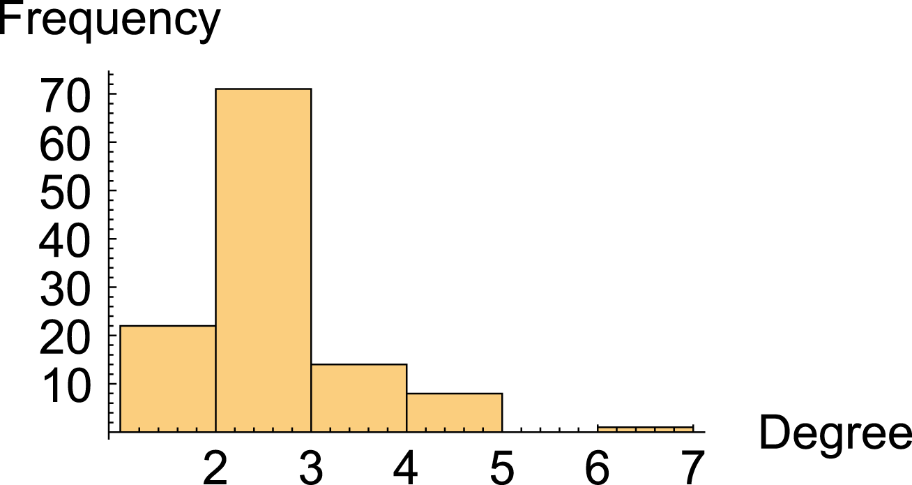
Figure 11. Degree distribution plot for behavioral network of simple drivetrain system.

Figure 12. Degree distribution plot for behavioral network of magnetic saturated inductor system.
In developing the behavioral networks for these systems, it was noted that there were some behaviors that existing modeling techniques could not handle. These behaviors had specific mathematical manifestations in the OpenModelica instantiation information. These mathematical constructs represent real behaviors in the real system. Therefore, modeling them correctly is critical. These modeling complexities were addressed before testing the hypothesis.
6.4 Modeling techniques
In this section, the modeling techniques developed in order to model more realistic systems are presented. First, a technique for modeling embedded behavior is presented. Then, a technique for modeling logical behavior is presented. With these techniques, systems with a wider range of behaviors can be modeled using BNA.
6.4.1 Modeling embedded behavior
An embedded function call represents embedded behavior. The function call may describe the behavior of a small sub-system or a mathematical tool in the governing equations used when a specific calculation needs to be performed several times. For instance, an embedded function could be used for converting a temperature in Celsius to a temperature in Kelvin. When these embedded functions are to be performed several times, each set of input parameters is unique, and therefore the output parameters of each function call are unique. In the governing equations, a function call occurs when an embedded function is defined and then referred to by at least one equation. An example is in (5)–(10). (5)–(9) comprise the function definition, while (10) demonstrates an equation calling the function. This example is from one of the systems used in the study. The embedded function definition may also include an algorithm to show how the output is calculated.
 $$\begin{eqnarray}\displaystyle & & \displaystyle \mathit{function}~\mathit{ToSpacePhasor}\end{eqnarray}$$
 $$\begin{eqnarray}\displaystyle & & \displaystyle \quad \mathit{input}~\mathit{Real}[3]~x;\end{eqnarray}$$
 $$\begin{eqnarray}\displaystyle & & \displaystyle \quad \mathit{output}~\mathit{Real}[2]~y;\end{eqnarray}$$
 $$\begin{eqnarray}\displaystyle & & \displaystyle \quad \mathit{output}~\mathit{Real}~y0;\end{eqnarray}$$
 $$\begin{eqnarray}\displaystyle & & \displaystyle \mathit{end}~\mathit{ToSpacePhasor};\end{eqnarray}$$
 $$\begin{eqnarray}\displaystyle & & \displaystyle F1:~(\mathit{electricalPowerSensor.i}\_,\_)=\mathit{ToSpacePhasor}\nonumber\\ \displaystyle & & \displaystyle \quad (\{\!\mathit{electricalPowerSensor.plug}\_p.\mathit{pin}[1].i,\nonumber\\ \displaystyle & & \displaystyle \quad \mathit{electricalPowerSensor.plug}\_p.\mathit{pin}[2].i,\nonumber\\ \displaystyle & & \displaystyle \quad \quad \mathit{electricalPowerSensor.plug}\_p.\mathit{pin}[3].i\!\});\end{eqnarray}$$
There are two outputs from the embedded function: $y$
and
$y$
and $y0$
. This is illustrated in (5)–(9). Because the outputs will be different depending on the inputs used, one cannot simply use those outputs every time the function is called. Otherwise, if the embedded function were used multiple times, the nodes associated with the outputs of the embedded function would have an inappropriately high node degree in the behavioral network. To handle this complexity, a new output parameter is created for each instance of the function being called. If the instantiation information has multiple function calls with different inputs, the name of the output must depend on the inputs used in the function call. The embedded function outputs for the function call are given in (11) and (12). To reiterate for clarity, embedded functions are not the same as the functions which are described by the governing equations of the system.
$y0$
. This is illustrated in (5)–(9). Because the outputs will be different depending on the inputs used, one cannot simply use those outputs every time the function is called. Otherwise, if the embedded function were used multiple times, the nodes associated with the outputs of the embedded function would have an inappropriately high node degree in the behavioral network. To handle this complexity, a new output parameter is created for each instance of the function being called. If the instantiation information has multiple function calls with different inputs, the name of the output must depend on the inputs used in the function call. The embedded function outputs for the function call are given in (11) and (12). To reiterate for clarity, embedded functions are not the same as the functions which are described by the governing equations of the system.
 $$\begin{eqnarray}\displaystyle & & \displaystyle y(\{\!\mathit{electricalPowerSensor.plug}\_p.\mathit{pin}[1].i,\nonumber\\ \displaystyle & & \displaystyle \quad \mathit{electricalPowerSensor.plug}\_p.\mathit{pin}[2].i,\nonumber\\ \displaystyle & & \displaystyle \quad \mathit{electricalPowerSensor.plug}\_p.\mathit{pin}[3].i\!\})\end{eqnarray}$$
 $$\begin{eqnarray}\displaystyle & & \displaystyle y0(\{\!\mathit{electricalPowerSensor.plug}\_p.\mathit{pin}[1].i,\nonumber\\ \displaystyle & & \displaystyle \quad \mathit{electricalPowerSensor.plug}\_p.\mathit{pin}[2].i,\nonumber\\ \displaystyle & & \displaystyle \quad \mathit{electricalPowerSensor.plug}\_p.\mathit{pin}[3].i\!\})\end{eqnarray}$$
The output parameters in (11) and (12), $\text{electricalPowerSensor.i}\_$
, and
$\text{electricalPowerSensor.i}\_$
, and $F1$
comprise the list of nodes describing (10). The underscore on the left-hand side of (10) is not a parameter node because it is not a design parameter. A new function node must be added for the function call in (10). This is
$F1$
comprise the list of nodes describing (10). The underscore on the left-hand side of (10) is not a parameter node because it is not a design parameter. A new function node must be added for the function call in (10). This is $F2$
. The nodes associated with
$F2$
. The nodes associated with $F2$
are the inputs and outputs of the function call. Figure 13 is the resulting network segment for this example.
$F2$
are the inputs and outputs of the function call. Figure 13 is the resulting network segment for this example.

Figure 13. Resulting network segment for function call example from SMEE generator system.
6.4.2 Modeling logical behavior
 $$\begin{eqnarray}\displaystyle & & \displaystyle \mathit{if}~\mathit{not}~\mathit{out}\_p.m\_\mathit{leakBEcurrentIsGiven}>0.5~\mathit{then}\end{eqnarray}$$
 $$\begin{eqnarray}\displaystyle & & \displaystyle \quad \mathit{out}\_p.m\_\mathit{leakBEcurrent}:=\nonumber\\ \displaystyle & & \displaystyle \quad \quad \mathit{out}\_p.m\_c2\times \mathit{out}\_p.m\_\mathit{satCur};\end{eqnarray}$$
 $$\begin{eqnarray}\displaystyle & & \displaystyle \mathit{end}~\mathit{if};\end{eqnarray}$$
Some systems included logical behavior, which shows up as discrete equations in the set of governing equations. An if-clause is one type of discrete equation. There is a relationship between the condition in the if-clause and the parameters contained in the body of the if-clause which cannot be ignored. All parameters in the body of the if-clause as well as the if-condition itself must be connected to a single function node. The same goes for parameters associated with an else-if or else statement.

Figure 14. Resulting network segment for if-clause example from electrical oscillator system.
An excerpt from the set of governing equations including an example of an if-clause is given in (13)–(15). Figure 14 shows the resulting network segment. Since all of the parameters in (13)–(15) are included in the same if statement, they are all connected to the same function node in the resulting network segment in Figure 14.
Other examples of discrete equations include when-clauses. There are also if-expressions and assert statements, which are handled the same as if they were structured as an if-clause. These modeling advances allowed all forty systems to be analyzed. In the next section, results of the empirical study are presented.
7 Results and analysis
In this section, the hypothesis tested whether the change in the network metric ASPL due to attack on parameter nodes is higher in bridging nodes, which are key structural elements of networks, than non-bridging nodes. To restate the method for testing the hypothesis, a fault variable was applied to all edges associated with each attacked parameter node. Then, the network metric was calculated and compared to the network metric calculated from nominal case, which is when no fault variable is applied to any edge in the network. A large $\unicode[STIX]{x0394}\text{ASPL}$
, or change in ASPL, for a particular node means that degradation of that node significantly impacts system-level performance. Bridging nodes were located by first finding communities in the network and then using the definition of bridging nodes to determine which parameter nodes in the network were bridging nodes. The results in Table 2 show the average
$\unicode[STIX]{x0394}\text{ASPL}$
, or change in ASPL, for a particular node means that degradation of that node significantly impacts system-level performance. Bridging nodes were located by first finding communities in the network and then using the definition of bridging nodes to determine which parameter nodes in the network were bridging nodes. The results in Table 2 show the average $\unicode[STIX]{x0394}\text{ASPL}$
for bridging and non-bridging nodes in a representative selection of systems. The full data set includes the average
$\unicode[STIX]{x0394}\text{ASPL}$
for bridging and non-bridging nodes in a representative selection of systems. The full data set includes the average $\unicode[STIX]{x0394}\text{ASPL}$
of bridging and non-bridging nodes for all forty systems and for two different community-finding algorithms. To determine whether or not the difference in average
$\unicode[STIX]{x0394}\text{ASPL}$
of bridging and non-bridging nodes for all forty systems and for two different community-finding algorithms. To determine whether or not the difference in average $\unicode[STIX]{x0394}\text{ASPL}$
is statistically significant, a one-tailed t-test was used. A one-tailed t-test is appropriate for this study because the hypothesis is about whether or not bridging nodes have a higher
$\unicode[STIX]{x0394}\text{ASPL}$
is statistically significant, a one-tailed t-test was used. A one-tailed t-test is appropriate for this study because the hypothesis is about whether or not bridging nodes have a higher $\unicode[STIX]{x0394}\text{ASPL}$
than non-bridging nodes, which developed as a result of the conceptual proof discussed earlier in this article. The results of the t-test, shown in Table 3, show that bridging nodes have a significantly higher
$\unicode[STIX]{x0394}\text{ASPL}$
than non-bridging nodes, which developed as a result of the conceptual proof discussed earlier in this article. The results of the t-test, shown in Table 3, show that bridging nodes have a significantly higher $\unicode[STIX]{x0394}\text{ASPL}$
than non-bridging nodes.
$\unicode[STIX]{x0394}\text{ASPL}$
than non-bridging nodes.
Table 2. $\unicode[STIX]{x0394}\text{ASPL}$
and bridging nodes: average
$\unicode[STIX]{x0394}\text{ASPL}$
and bridging nodes: average $\unicode[STIX]{x0394}\text{ASPL}$
of bridging parameter nodes and non-bridging parameter nodes in a representative selection of systems
$\unicode[STIX]{x0394}\text{ASPL}$
of bridging parameter nodes and non-bridging parameter nodes in a representative selection of systems

Table 3. $\unicode[STIX]{x0394}\text{ASPL}$
and bridging nodes: t-test results
$\unicode[STIX]{x0394}\text{ASPL}$
and bridging nodes: t-test results

In all systems studied, bridging nodes had a higher $\unicode[STIX]{x0394}\text{ASPL}$
on average than non-bridging nodes. This tendency is robust to different community-finding algorithms, of which there are many (Newman Reference Newman2004). To show this, the t-test is performed with bridging nodes found using two different community-finding algorithms, modularity maximization and spectral. The spectral algorithm partitions the graph using information about eigenvectors and eigenvalues of the adjacency matrix of the graph. See the
$\unicode[STIX]{x0394}\text{ASPL}$
on average than non-bridging nodes. This tendency is robust to different community-finding algorithms, of which there are many (Newman Reference Newman2004). To show this, the t-test is performed with bridging nodes found using two different community-finding algorithms, modularity maximization and spectral. The spectral algorithm partitions the graph using information about eigenvectors and eigenvalues of the adjacency matrix of the graph. See the $\unicode[STIX]{x0394}\text{ASPL}$
values from a representative selection of systems using both community-finding methods in Table 2. The results of the t-test are given in Table 3. These results show that the difference between the average
$\unicode[STIX]{x0394}\text{ASPL}$
values from a representative selection of systems using both community-finding methods in Table 2. The results of the t-test are given in Table 3. These results show that the difference between the average $\unicode[STIX]{x0394}\text{ASPL}$
is statistically significant (
$\unicode[STIX]{x0394}\text{ASPL}$
is statistically significant ( $p<0.01$
for both community-finding algorithms) and the effect sizes are strong and moderate for modularity maximization and spectral methods, respectively. This means that the presence of bridging nodes has a moderate to strong effect on the failure tolerance of the system. Table 4 shows the standard deviation measures for each community-finding algorithm for both bridging and non-bridging nodes. Unsurprisingly, the standard deviation does not change significantly between community-finding algorithms. For bridging nodes, one would need more than four digits of accuracy to notice a difference between the modularity maximization and spectral methods.
$p<0.01$
for both community-finding algorithms) and the effect sizes are strong and moderate for modularity maximization and spectral methods, respectively. This means that the presence of bridging nodes has a moderate to strong effect on the failure tolerance of the system. Table 4 shows the standard deviation measures for each community-finding algorithm for both bridging and non-bridging nodes. Unsurprisingly, the standard deviation does not change significantly between community-finding algorithms. For bridging nodes, one would need more than four digits of accuracy to notice a difference between the modularity maximization and spectral methods.

Figure 15. Behavioral network for simple drive train with grounded elements with edges associated with most vulnerable parameter node darkened and communities circled.
Table 4. $\unicode[STIX]{x0394}\text{ASPL}$
and bridging nodes: standard deviation
$\unicode[STIX]{x0394}\text{ASPL}$
and bridging nodes: standard deviation

In addition to these numerical results, the behavioral networks for all forty systems studied were graphed in Mathematica for visualization purposes. A few examples are shown in Figures 15–18. Communities, as determined by a modularity maximization community detection algorithm, are circled. The edges associated with the parameter node with the highest $\unicode[STIX]{x0394}\text{ASPL}$
are marked with a thicker line. It is clear that in all four cases at least one of the edges associated with this parameter node connects communities, meaning that this parameter node is a bridging node. In general, a parameter node needs only one edge connecting community to be considered a bridging node. In these figures, the parameter node with the highest
$\unicode[STIX]{x0394}\text{ASPL}$
are marked with a thicker line. It is clear that in all four cases at least one of the edges associated with this parameter node connects communities, meaning that this parameter node is a bridging node. In general, a parameter node needs only one edge connecting community to be considered a bridging node. In these figures, the parameter node with the highest $\unicode[STIX]{x0394}\text{ASPL}$
is highlighted to show that parameter nodes with high
$\unicode[STIX]{x0394}\text{ASPL}$
is highlighted to show that parameter nodes with high $\unicode[STIX]{x0394}\text{ASPL}$
are frequently bridging nodes. This is based on the results of the hypothesis test. BNA, however, assigns a value of
$\unicode[STIX]{x0394}\text{ASPL}$
are frequently bridging nodes. This is based on the results of the hypothesis test. BNA, however, assigns a value of $\unicode[STIX]{x0394}\text{ASPL}$
to each parameter node, thus giving a ranking of parameter nodes from most to least vulnerable.
$\unicode[STIX]{x0394}\text{ASPL}$
to each parameter node, thus giving a ranking of parameter nodes from most to least vulnerable.

Figure 16. Behavioral network for electrical rectifier circuit with edges associated with most vulnerable parameter node darkened and communities circled.
8 Determining the effect of the fault variable value
An unanswered question from previous work in BNA (Haley et al. Reference Haley, Dong and Tumer2014, Reference Haley, Dong and Tumer2016) was the effect of the value of the fault variable used when attacking nodes. To answer this question, a study on the effect of the value of the fault variable on the results of the ASPL of behavioral networks is presented. The fault variable, as discussed, is the value applied to the edge weights of the edges associated with a given parameter node when it is under attack. The fault variable was given a value of 0.5 consistently in the previously shown experiments. However, the effects of changing this value have not been considered. The BNA is repeated for fault variable values of 0.2, 0.5, 0.7, and 0.9 and the results are compared.

Figure 17. Elasto gap behavioral network with edges associated with most vulnerable parameter node darkened and communities circled.
The results in Figure 19 show that the average $\unicode[STIX]{x0394}\text{ASPL}$
of all parameter nodes within a system decreases approximately linearly as the fault variable value increases. However, the sorted list of systems from smallest to largest average
$\unicode[STIX]{x0394}\text{ASPL}$
of all parameter nodes within a system decreases approximately linearly as the fault variable value increases. However, the sorted list of systems from smallest to largest average $\unicode[STIX]{x0394}\text{ASPL}$
is unchanged regardless of which value is used for the fault variable. In other words, the value of the fault variable does not affect which parameter nodes are considered the most vulnerable in the system.
$\unicode[STIX]{x0394}\text{ASPL}$
is unchanged regardless of which value is used for the fault variable. In other words, the value of the fault variable does not affect which parameter nodes are considered the most vulnerable in the system.

Figure 18. Control temperature of a resistor behavioral network with edges associated with most vulnerable parameter node darkened and communities circled.

Figure 19. Effect of fault variable value on average $\unicode[STIX]{x0394}\text{ASPL}$
in each system.
$\unicode[STIX]{x0394}\text{ASPL}$
in each system.
9 Discussion
The role of bridging nodes in behavioral network models of engineering systems had not previously been explored. In this article, it was found that bridging nodes, under degradation, yield a larger change in the network metric ASPL based on previous network-metric-based methods presented for BNA (Haley et al. Reference Haley, Dong and Tumer2014, Reference Haley, Dong and Tumer2016). This finding highlights the structural role of vulnerable parameter nodes, which, despite the well-documented relationship between a network’s structure and its ability to withstand attack (Sha and Panchal Reference Sha and Panchal2013), had not previously been studied. It is important to note that this is a statistical observation. Bridging nodes tend to be associated with a larger system-level degradation. This statistical finding holds even when those bridging nodes have a low degree of connectivity compared to non-bridging nodes that may have a high degree of connectivity, such as to nodes within its community. The important finding is thus that engineers should pay attention to nodes that sit between communities and not necessarily high-degree nodes that sit within communities. The failure of the former may cause more significant system-level faults whereas the failure of the latter could be isolated within the community so long as the bridging node is not degraded.
The importance of network structure is well known and has been well researched (Braha and Bar-Yam Reference Braha and Bar-Yam2004), and behavioral networks should be no exception. Because of the relationship between bridging nodes and the community structure of a network, this finding leads to the examination of the relationship between bridging nodes and modularity in behavioral networks, setting the stage for future work. For example, increasing modularity is generally recommended as one approach to improve the robustness of a system. Future research could test the extent to which increasing robustness through modularity is mediated by the presence of bridging nodes.
In addition, advances to the modeling methods presented in previous work in BNA (Haley et al.
Reference Haley, Dong and Tumer2014, Reference Haley, Dong and Tumer2016) were developed. Inadequate modeling capabilities would prevent real engineering systems from being modeled in BNA. Specifically, these modeling advances included the ability to model logic and embedded behavior. This work also analyzed the robustness of the method using network metrics to different values of the fault variable. Since the $\unicode[STIX]{x0394}\text{ASPL}$
values are already small in magnitude, it is reasonable to choose a relatively small or moderate value of the fault variable so that
$\unicode[STIX]{x0394}\text{ASPL}$
values are already small in magnitude, it is reasonable to choose a relatively small or moderate value of the fault variable so that $\unicode[STIX]{x0394}\text{ASPL}$
can be measured accurately without using excessively small numbers. From the data gathered in this study, both 0.2 and 0.5 could be considered good choices for the fault variable value. More important than the chosen value of the fault variable, however, is the fact that it must be consistent across all node failures within a system. Since the value of the fault variable affects the numerical value of
$\unicode[STIX]{x0394}\text{ASPL}$
can be measured accurately without using excessively small numbers. From the data gathered in this study, both 0.2 and 0.5 could be considered good choices for the fault variable value. More important than the chosen value of the fault variable, however, is the fact that it must be consistent across all node failures within a system. Since the value of the fault variable affects the numerical value of $\unicode[STIX]{x0394}\text{ASPL}$
, the same value must be used for the fault variable when comparing node failures within a system.
$\unicode[STIX]{x0394}\text{ASPL}$
, the same value must be used for the fault variable when comparing node failures within a system.
10 Conclusions
In conclusion, this article presented conceptual and empirical arguments showing that existing network-metric-based methods used for BNA correlate with bridging nodes in the behavioral network. This finding has implications regarding the community structure of behavioral networks and gives the designer a priori predictions on vulnerable parameters. Moreover, this article showed that the method for faulting behavioral networks is robust to different values of the fault variable and presented new modeling techniques to be able to analyze more realistic systems. All of these findings contribute to the research community’s understanding of BNA and of network analysis of engineering systems as a whole.
Once fully developed, the BNA method can be used in early design stages and can avoid a full-scale behavioral simulation. The results of BNA lead to an understanding of the design parameters for which failure could cause large degradation in system-level performance. Based on knowledge of vulnerable parameters based on the results of the BNA method, system designers can specify tight manufacturing tolerances or add sensors. Making these kinds of changes earlier in the design process can reduce cost and create safer systems in the future.
11 Future work
Behavioral models are useful in early design stages but are ultimately only part of the picture. For later stages of design, the behavioral model must be interfaced with a component model of the system. Both types of models are necessary for a complete understanding of the engineering system. While behavioral models are useful in early stages of design, if failure probabilities are required later in the design process, this method may not be appropriate. Future work will aim to implement BNA for an in-depth case study to test how BNA would work on a real system.
So far the authors have only used governing equations from OpenModelica instantiation information to build behavioral networks. It is unclear whether different sets of governing equations describing the system have a significant impact on the results of BNA. For instance, there are different theories that can be used to describe the same natural phenomenon. Future work will examine the effects of using these different sets of equations and whether or not the granularity of these equations is of particular importance.
This article has shown that parameters associated with bridging nodes, which connect communities, are key to understanding the failure tolerance of engineering systems. These communities group together closely related parameter nodes which relate to a particular behavior. It is likely that these communities in the behavioral network relate to the modularity of the system. It is also possible that these behavioral modules could indicate long distance relationships between parameters which create unexpected sub-system interactions. These questions belong to future work. Specifically, future work will test whether or not communities in the behavioral network reflect meaningful system behaviors and associations between parameters. For this research to be possible, future work will investigate more closely how using different sets of physics equations affects the results of the BNA.
Financial Support
This research is supported by the National Science Foundation (NSF CMMI-1562027). Any opinions or findings of this work are the responsibility of the authors and do not necessarily reflect the views of the sponsors or collaborators.
Appendix A. Description of systems used in study


 Open access