


1. Introduction
Consider a person who must drive home after visiting a friend. On the highway there are two exits, and to reach his house he must leave the highway at the second exit. However, since he is absentminded, he cannot remember at the second exit whether he saw the first exit or not. As both exits look alike, he does not know at which of the two exits he is when he sees one. If he leaves the highway at the first exit he will enter a scary road – somewhere he would much rather not spend the night. If, on the other hand, he continues at the second exit then he arrives at a motel. He clearly prefers to sleep at home rather than spending the night at the motel. This situation is visually depicted in Figure 1.

Figure 1. The absentminded driver problem.
The question is: What should the driver do when he sees an exit? Continue or leave the highway, or perhaps even randomize over these two options? This is known as the paradox of the absentminded driver, or simply the absentminded driver problem.
Ever since its introduction by Piccione and Rubinstein (Reference Piccione and Rubinstein1997), the absentminded driver problem has provoked lively discussions and controversy among game theorists, decision theorists, logicians, philosophers, computer scientists and economists. The problem seems thought provoking for several reasons.
First, it stands apart from traditional one-person decision problems under uncertainty, as in most of its existing formulations the independence between acts and states is violated, and the states are not mutually exclusive. Indeed, upon reaching an exit on the highway, the absentminded driver is uncertain whether this is the first or second exit, but his act of whether or not to take the exit influences the probability of reaching the second exit. Hence, if the states merely represent the two exits, then the act chosen influences the likelihood of the two states. Moreover, the states would also not be mutually exclusive in this case, because reaching the second exit implies that the first exit must have been reached previously. This poses a problem for how the driver must update his beliefs upon seeing an exit.
Second, there seems to be a tension between planning the decision ex ante, and implementing the decision once the driver is on the highway. Most of the existing papers find that the ex ante optimal probability of leaving the highway is no longer optimal if the driver really sees the exit, and updates his beliefs accordingly. This presents a serious problem.
In this paper we present two possible resolutions to the problem. In the first, we assume that the driver can reason about his degree of absentmindedness before making a decision. More precisely, the driver contemplates the possibilities that he would be absentminded only at the first exit, only at the second exit, at both exits or at no exit. These four states are mutually exclusive, and restore the act-state independence. This allows us to undertake a traditional Savage-style analysis (Savage Reference Savage1972). In particular, we find that the tension between ex ante planning and optimal choice on the highway disappears.
In our second scenario, we assume that the states do not merely correspond to the two exits, but represent the three possible final destinations indexed by time. Assuming there are two time periods (the time when the first exit would appear, and the time when the second exit would appear), this results in six possible centred states. Moreover, the six states would be mutually exclusive (but act-state independence would still be violated). If the driver sees an exit, then he must rule out the centred state where the first exit has been taken and the time period is 2. We find that, upon revising the belief by Bayesian updating, the optimal probability of continuing when seeing an exit is approximately 0.53. This is different from most papers in the literature which point at an optimal continuation probability of ${2 \over 3}$
. We also show that adopting our solution is the only way in which the driver can be immune to diachronic Dutch strategies.
${2 \over 3}$
. We also show that adopting our solution is the only way in which the driver can be immune to diachronic Dutch strategies.
The outline of the paper is as follows. In section 2, we present the time consistency issue that is at the heart of the absent-minded driver problem. In sections 3 and 4 we analyse the absentminded driver problem using the two different scenarios described above. In section 5, we analyse when the driver would be immune to Dutch strategies, showing that he can avoid a Dutch strategy only if he follows our proposed solution. In section 6 we discuss other approaches to the absentminded driver problem in the literature, and then consider the implications of our solution for time consistency in section 7. Section 8 concludes.
2. The Time Consistency Problem
Piccione and Rubinstein (Reference Piccione and Rubinstein1997) point out that there seems to be a tension between optimal planning and time consistency in the absentminded driver problem. Suppose the driver must plan what to do before he leaves the house of his friend. Since he cannot make his choice conditional on reaching the first or second exit, a strategy would simply be: continue if you see an exit, leave the highway if you see an exit, or possibly a randomization over these two possibilities. Let us first focus on the case without randomization. Then, the best strategy from an ex ante perspective would be to continue if you see an exit. Now, suppose the driver finds himself on the highway and sees an exit. Given his strategy to always continue, it seems reasonable for him to believe that he is at the first exit with probability 0.5. But then, the expected utility of leaving the highway would be 2, which is more than what he would get by continuing. Hence, the driver would be tempted to change his plan once he finds himself on the highway. In other words, the optimal plan from the ex ante perspective is not time consistent.
This tension between optimal planning and time consistency will persist if we allow for randomization. Suppose the driver plans to use the same randomization device every time he sees an exit, which induces him to continue with probability $\pi $
and to leave with probability
$\pi $
and to leave with probability $1 - \pi $
at both exits. Then, the ex ante expected utility from this plan would be
$1 - \pi $
at both exits. Then, the ex ante expected utility from this plan would be ${\pi ^2} \cdot 1 + \pi (1 - \pi ) \cdot 4 + (1 - \pi ) \cdot 0$
, which is maximized when
${\pi ^2} \cdot 1 + \pi (1 - \pi ) \cdot 4 + (1 - \pi ) \cdot 0$
, which is maximized when $\pi = {2 \over 3}$
. Suppose again that the driver finds himself on the highway and sees an exit, and let
$\pi = {2 \over 3}$
. Suppose again that the driver finds himself on the highway and sees an exit, and let $\beta $
be the probability that he assigns to being at the first exit. Given his strategy, it seems reasonable for him to believe that the probability of being at the second exit is
$\beta $
be the probability that he assigns to being at the first exit. Given his strategy, it seems reasonable for him to believe that the probability of being at the second exit is $\beta \cdot {2 \over 3}$
, which means that
$\beta \cdot {2 \over 3}$
, which means that $\beta = 0.6$
. Given these beliefs, however, the expected utility of leaving the highway is higher than that of continuing, and hence the driver would again be tempted to change his plan to leaving the highway with probability 1. That is, the probabilistic ex ante optimal plan is not time consistent, either.
$\beta = 0.6$
. Given these beliefs, however, the expected utility of leaving the highway is higher than that of continuing, and hence the driver would again be tempted to change his plan to leaving the highway with probability 1. That is, the probabilistic ex ante optimal plan is not time consistent, either.
Existing approaches to the absent-minded problem in the literature all try to resolve the time-consistency issue, but present serious drawbacks, which we will discuss in more detail below (see section 6): either (i) act-state independence is violated; or (ii) the states are not mutually exclusive; or finally (iii) the driver is separated into two agents that choose independently. As a consequence, none of these approaches can be fully reconciled with the standard Savage (Reference Savage1972) framework. In the next section, we present an alternative proposal where a minimal reformulation of the problem allows us to avoid all of these issues, making it consistent with the Savage framework.
A common feature among the approaches in the literature is what we will call the ‘no news assumption’ (also called no news, no change assumption in Baratgin and Walliser (Reference Baratgin and Walliser2010)), i.e. that the driver does not learn any new information upon reaching an exit. We challenge this assumption in the following two sections, and use this to motivate two alternative approaches in these sections. In the first scenario we present a framework that restores the act-state independence in Savage (Reference Savage1972). The second scenario still violates act-state independence, and thus requires a revision of the Savage framework, but we argue that the reasoning supporting our solution there is independently plausible and better motivated than other alternatives.
3. Reasoning about Your Degree of Absentmindedness
In this section we offer an alternative approach that is completely in line with the Savage set-up. We do not explicitly incorporate time into our analysis, but rather allow the driver to reason about his degree of absentmindedness. This will enable us to provide a Savage-style model in which the events about which the driver is uncertain at the ex ante stage are mutually exclusive, and where the driver’s possible acts – to continue or to leave the highway at an exit – do not influence the state. Moreover, the driver is not separated into different agents.
More precisely, at the ex ante stage the driver believes that he may either be absentminded (i) at no exit, (ii) at the first exit only, (iii) at the second exit only, or (iv) at both exits. If the driver is absentminded at an exit then, as a consequence, he will continue at this exit even if he planned to leave there, and he will forget about this exit for the remainder of the journey. Moreover, the driver is perfectly aware of this before he starts the journey. The four mutually exclusive events listed above correspond to the states ${\omega _0},{\omega _1},{\omega _2}$
and
${\omega _0},{\omega _1},{\omega _2}$
and ${\omega _{12}}$
, respectively. The decision problem at the ex ante stage may therefore be summarized by Table 1.
${\omega _{12}}$
, respectively. The decision problem at the ex ante stage may therefore be summarized by Table 1.
Table 1. Reasoning about your degree of absentmindedness

To understand the consequences of the various acts at the different states, assume first that the driver chooses to continue. Then, no matter what the state is, he would always continue at every exit he reaches, either because he wants to, or because he is absentminded at that exit, which automatically makes him continue there. As a consequence, he would certainly reach the motel.
Suppose next that the driver plans to leave, and that the state is either ${\omega _0}$
or
${\omega _0}$
or ${\omega _2}$
, that is, the driver is not absentminded at the first exit. Then he would already leave at the first exit, since he is not absentminded there, and reach the scary road.
${\omega _2}$
, that is, the driver is not absentminded at the first exit. Then he would already leave at the first exit, since he is not absentminded there, and reach the scary road.
Now assume that the driver plans to leave and the state is ${\omega _1}$
, which means that he is absentminded at the first, but not at the second, exit. Then, he would continue at the first exit since he is absentminded there, but leave at the second exit, at which he is not absentminded. As a result, he would reach his home.
${\omega _1}$
, which means that he is absentminded at the first, but not at the second, exit. Then, he would continue at the first exit since he is absentminded there, but leave at the second exit, at which he is not absentminded. As a result, he would reach his home.
Finally, suppose that the driver plans to leave and the state is ${\omega _{12}}$
, meaning that the driver is absentminded at both exits. Then, he would still continue at both exists since he is absentminded at both of these. As a consequence, he would reach the motel.
${\omega _{12}}$
, meaning that the driver is absentminded at both exits. Then, he would still continue at both exists since he is absentminded at both of these. As a consequence, he would reach the motel.
The states in our model are fundamentally different from those in Schwarz (Reference Schwarz2015). In the latter paper, the state describes the exit at which the driver currently finds himself, and, in case he is at the first exit, a description of what the driver would do at the second exit in case it is reached. In our set-up, the state merely describes the exit(s) at which he believes to be absentminded. It does not describe at which exit he is, nor what he would do at the second exit. In fact, the latter is determined by the combination of his act and his state of absentmindedness at the second exit.
Note that in our model there is no dependence between acts and states. Indeed, the plan to continue or not at an exit has no influence on the fact whether the driver is absentminded at a particular exit or not. Let $P(\omega )$
denote the prior probability that the driver assigns to state
$P(\omega )$
denote the prior probability that the driver assigns to state $\omega $
at the ex ante stage. Then, the ex ante expected utilities of continue and leave would be
$\omega $
at the ex ante stage. Then, the ex ante expected utilities of continue and leave would be $EU(cont) = 1$
and
$EU(cont) = 1$
and $EU(leave) = 4P({\omega _1}) + 1P({\omega _{12}})$
, respectively. Hence, from an ex ante perspective it is optimal for the driver to leave the highway at an exit precisely when
$EU(leave) = 4P({\omega _1}) + 1P({\omega _{12}})$
, respectively. Hence, from an ex ante perspective it is optimal for the driver to leave the highway at an exit precisely when $4P({\omega _1}) + P({\omega _{12}}) 1$
, that is, when he deems it sufficiently likely that he will be absentminded at the first exit but not at the second one.
$4P({\omega _1}) + P({\omega _{12}}) 1$
, that is, when he deems it sufficiently likely that he will be absentminded at the first exit but not at the second one.
Now assume that $P({\omega _{12}}) \lt 1$
, the driver sees an exit, and reasons about whether to leave or not. Then he must conclude that he is not absentminded at both exits, and hence
$P({\omega _{12}}) \lt 1$
, the driver sees an exit, and reasons about whether to leave or not. Then he must conclude that he is not absentminded at both exits, and hence ${\omega _{12}}$
is no longer possible. If he uses general Bayesian updating with respect to the event
${\omega _{12}}$
is no longer possible. If he uses general Bayesian updating with respect to the event $E = \{ {\omega _0},{\omega _1},{\omega _2}\} $
to revise his prior belief, then his updated belief
$E = \{ {\omega _0},{\omega _1},{\omega _2}\} $
to revise his prior belief, then his updated belief $P( \cdot |E)$
will be given by
$P( \cdot |E)$
will be given by
 $$P({\omega _0}|E) = {{P({\omega _0})} \over {1 - P({\omega _{12}})}},P({\omega _1}|E) = {{P({\omega _1})} \over {1 - P({\omega _{12}})}},P({\omega _2}|E) = {{P({\omega _2})} \over {1 - P({\omega _{12}})}}.$$
Hence, it will still be optimal to leave the highway at an exit precisely when $4P({\omega _1}) + P({\omega _{12}}) 1$
, just like at the ex ante stage. In other words, there is no time inconsistency in this model.
$4P({\omega _1}) + P({\omega _{12}}) 1$
, just like at the ex ante stage. In other words, there is no time inconsistency in this model.
Indeed, if the driver sees an exit, then he receives the informative message that the state ${\omega _{12}}$
, at which he would be absentminded at both exits, is no longer possible. The evidence received in this model is thereby uncentred, because it does not reveal anything about the time period. However, this feature does not play an essential role in our analysis here. The message received could, in principle, be a reason for revising his optimal plan, but in this case the driver will stick to the optimal plan he chose before receiving the message.
${\omega _{12}}$
, at which he would be absentminded at both exits, is no longer possible. The evidence received in this model is thereby uncentred, because it does not reveal anything about the time period. However, this feature does not play an essential role in our analysis here. The message received could, in principle, be a reason for revising his optimal plan, but in this case the driver will stick to the optimal plan he chose before receiving the message.
The deeper reason for why the driver’s preferences before and after seeing an exit remain the same lies in Savage’s sure-thing principle. This principle states that, whenever the decision maker chooses the same optimal plan, no matter whether an event E is realized or not, then the decision maker must also choose that same optimal plan without knowing whether E is realized or not. Now, take the event E to be the state ${\omega _{12}}$
. Clearly, if the driver knows that
${\omega _{12}}$
. Clearly, if the driver knows that ${\omega _{12}}$
applies, then he would be indifferent between his two choices, as both would lead him to the motel. In particular, both choices are optimal for the driver if he knows that the state is
${\omega _{12}}$
applies, then he would be indifferent between his two choices, as both would lead him to the motel. In particular, both choices are optimal for the driver if he knows that the state is ${\omega _{12}}$
. Suppose, without loss of generality, that the driver would prefer to continue if he knows that
${\omega _{12}}$
. Suppose, without loss of generality, that the driver would prefer to continue if he knows that ${\omega _{12}}$
does not apply. As continuing is also optimal for the driver if he knows that
${\omega _{12}}$
does not apply. As continuing is also optimal for the driver if he knows that ${\omega _{12}}$
applies, it follows by the sure-thing principle that the driver would still (weakly) prefer to continue before he knows whether
${\omega _{12}}$
applies, it follows by the sure-thing principle that the driver would still (weakly) prefer to continue before he knows whether ${\omega _{12}}$
applies or not. In other words, his optimal choice before and after seeing an exit would be the same. This is in sharp contrast with many of the existing approaches, which do lead to decisions that are time inconsistent.
${\omega _{12}}$
applies or not. In other words, his optimal choice before and after seeing an exit would be the same. This is in sharp contrast with many of the existing approaches, which do lead to decisions that are time inconsistent.
Important in our model is that the driver, upon seeing an exit, learns that he cannot be absentminded at both exits, and thus that the state ${\omega _{12}}$
is no longer possible. In other words, the driver receives an informative message when seeing an exit, which means that the no news, no change assumption does not apply. The rationality criterion of no news, no change in Baratgin and Walliser (Reference Baratgin and Walliser2010) asserts that the decision maker should not change his beliefs if no relevant news comes in. This criterion is implied by the principle of strict conditionalization in Teller (Reference Teller1973), but also by temporal conditionalization in Talbott (Reference Talbott1991), which states that a belief is updated in Bayesian way if and only if a new message is received. It also follows from the strong conservation principle in Walliser and Zwirn (Reference Walliser and Zwirn2002), which stipulates that when a message is already known according to the prior probability, then the posterior probability must remain unchanged.
${\omega _{12}}$
is no longer possible. In other words, the driver receives an informative message when seeing an exit, which means that the no news, no change assumption does not apply. The rationality criterion of no news, no change in Baratgin and Walliser (Reference Baratgin and Walliser2010) asserts that the decision maker should not change his beliefs if no relevant news comes in. This criterion is implied by the principle of strict conditionalization in Teller (Reference Teller1973), but also by temporal conditionalization in Talbott (Reference Talbott1991), which states that a belief is updated in Bayesian way if and only if a new message is received. It also follows from the strong conservation principle in Walliser and Zwirn (Reference Walliser and Zwirn2002), which stipulates that when a message is already known according to the prior probability, then the posterior probability must remain unchanged.
4. Reasoning with Centred Possibilities
The solution we discussed in the previous section relies on a reformulation of the absentminded driver problem. In the original story, the driver knows that he will forget having passed any exit, even though he is aware of being at an exit at the time he reaches it. The second solution that we now turn to explore keeps the original formulation of the problem, and addresses one of the two concerns that we identified: namely, that in the formulation of the problem, the states are not mutually exclusive.
We begin by observing that there are three possible histories, terminating at the Motel $(A)$
, at Home
$(A)$
, at Home $(B)$
, or at the Scary road
$(B)$
, or at the Scary road $(C)$
, and the probability of each of these histories can be expressed in terms of the probability
$(C)$
, and the probability of each of these histories can be expressed in terms of the probability $\pi $
that the driver continues at each time he arrives at an exit (Table 2).
Footnote 1
$\pi $
that the driver continues at each time he arrives at an exit (Table 2).
Footnote 1
Table 2. The uncentred worlds model

If the utility of each history is: $U(A) = 1$
,
$U(A) = 1$
, $U(B) = 4$
,
$U(B) = 4$
, $U(C) = 0$
, then the expected utility is maximized at
$U(C) = 0$
, then the expected utility is maximized at $\pi = {2 \over 3}$
. However, this way of representing the problem does not take into account the driver’s uncertainty about what the time period is (and therefore what exit he is approaching). But, of course, this makes a difference to what the driver should do: if he is at the first exit, then he should prefer to continue, while if he is at the second exit, then he should exit. We cannot express what exit the driver is approaching using the model in Table 2, since that does not model the different time periods at which the driver could be located. In other words, the simple model in Table 2 does not capture one important dimension of the driver’s uncertainty, that is which time period he is at.
$\pi = {2 \over 3}$
. However, this way of representing the problem does not take into account the driver’s uncertainty about what the time period is (and therefore what exit he is approaching). But, of course, this makes a difference to what the driver should do: if he is at the first exit, then he should prefer to continue, while if he is at the second exit, then he should exit. We cannot express what exit the driver is approaching using the model in Table 2, since that does not model the different time periods at which the driver could be located. In other words, the simple model in Table 2 does not capture one important dimension of the driver’s uncertainty, that is which time period he is at.
To address this issue, we enrich the model to add the driver’s time location. This will allow us to represent the driver’s uncertainty regarding both the history and the time period at which he is located. The resulting refined model is summarized in Table 3.
Table 3. The centred world model
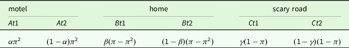
As before, $\pi $
represents the probability that the driver continues when reaching an exit, which we call the driver’s ‘choice probability’, and it determines the overall probability of each possible complete history (as before, A for the history ending at the motel, B for the one ending at home, and C for the one ending up at the scary road). In addition to the choice probability, we add parameters to capture the driver’s uncertainty about the time period. Since we are interested in the driver’s decisions at two successive points, we focus on two times:
$\pi $
represents the probability that the driver continues when reaching an exit, which we call the driver’s ‘choice probability’, and it determines the overall probability of each possible complete history (as before, A for the history ending at the motel, B for the one ending at home, and C for the one ending up at the scary road). In addition to the choice probability, we add parameters to capture the driver’s uncertainty about the time period. Since we are interested in the driver’s decisions at two successive points, we focus on two times: $t1$
for when the driver reaches the first exit, and
$t1$
for when the driver reaches the first exit, and $t2$
for when he either reaches the second exit or is on the way to the scary road, having already taken the first exit at
$t2$
for when he either reaches the second exit or is on the way to the scary road, having already taken the first exit at $t1$
. It is important to note that
$t1$
. It is important to note that $t1$
and
$t1$
and $t2$
in our model refer to time periods, not spatial locations, as the spatial location of the driver can indeed be different, at the same time point, for different histories. This gives rise to six centred possibilities, represented in Table 3. In this model, the states represent centred possibilities that are identified by a time point and the history within which they are located. So, for instance,
$t2$
in our model refer to time periods, not spatial locations, as the spatial location of the driver can indeed be different, at the same time point, for different histories. This gives rise to six centred possibilities, represented in Table 3. In this model, the states represent centred possibilities that are identified by a time point and the history within which they are located. So, for instance, $At2$
is the centred possibility where the driver is at
$At2$
is the centred possibility where the driver is at $t2$
and within the history ends up at the motel,
$t2$
and within the history ends up at the motel, $Bt2$
is the centred possibility where the driver is at
$Bt2$
is the centred possibility where the driver is at $t2$
and within the history ends up at home, and
$t2$
and within the history ends up at home, and $Ct2$
is the centred possibility where the driver is at
$Ct2$
is the centred possibility where the driver is at $t2$
and within the history ending at the scary road. In this model,
$t2$
and within the history ending at the scary road. In this model, $\alpha $
,
$\alpha $
, $\beta $
and
$\beta $
and $\gamma $
stand for the probability that it is time
$\gamma $
stand for the probability that it is time $t1$
, given that we are in history
$t1$
, given that we are in history $A,B$
or C, respectively. We can imagine that this is set on the basis of some randomizing mechanism by nature, where both of the time points within each history have equal probability. From now on, unless otherwise noted, we will assume that
$A,B$
or C, respectively. We can imagine that this is set on the basis of some randomizing mechanism by nature, where both of the time points within each history have equal probability. From now on, unless otherwise noted, we will assume that $\alpha = \beta = \gamma = {1 \over 2}$
.
Footnote 2
$\alpha = \beta = \gamma = {1 \over 2}$
.
Footnote 2
When the driver approaches an exit, the only thing he learns is that he hasn’t yet reached the Scary Road; in other words, he learns that it is not the second time period in history C, as otherwise he would have already abandoned the highway and reached the Scary Road. Out of the six possible centred locations, only five are compatible with his current evidence as he approaches the exit. He could be at the first time period, in which case each of the three histories is possible, as he could ultimately reach any of the final destinations depending on his next choices. Or he may already be at the second time period, and in this case he’d be on the road to either Home or the Motel, but certainly not the Scary Road, since he would have already passed that exit. We can represent the driver’s evidence set, as he approaches an exit, as the set $E = \{ At1,At2,Bt1,Bt2,Ct1\} $
.
$E = \{ At1,At2,Bt1,Bt2,Ct1\} $
.
The model in Table 2 did not allow us to formulate questions concerning which time period the driver is located at. But relative to the model in Table 3 we can now calculate the probability that the driver is at the first time period, and so approaching the first exit:
 $$Pr(t1|E) = {{Pr(t1\& E)} \over {Pr(E)}} = {{1/2} \over {{{1 - \pi } \over 2} + \pi }} = {1 \over {1 + \pi }}$$
Note that $Pr(t1|E) = 1/2$
only if
$Pr(t1|E) = 1/2$
only if $\pi = 1$
, so only if the driver is certain to continue at each exit the probability of being at the first one is
$\pi = 1$
, so only if the driver is certain to continue at each exit the probability of being at the first one is $1/2$
. But we cannot fix the probability of being at the first exit without knowing the value of
$1/2$
. But we cannot fix the probability of being at the first exit without knowing the value of $\pi $
, given that the driver is absentminded.
$\pi $
, given that the driver is absentminded.
As $\pi $
represents the choice probability, which is decided when the driver reaches an exit, its value is fixed then.
Footnote 3
At the time of choice, that is when he reaches an exit and his evidence is E, the driver should fix a value of
$\pi $
represents the choice probability, which is decided when the driver reaches an exit, its value is fixed then.
Footnote 3
At the time of choice, that is when he reaches an exit and his evidence is E, the driver should fix a value of $\pi = x$
that maximizes expected utility, given the payoffs associated with each history:
$\pi = x$
that maximizes expected utility, given the payoffs associated with each history:
 $$E{U_E}(\pi = x) = P{r_E}(A|\pi = x)U(A) + P{r_E}(B|\pi = x)U(B) + P{r_E}(C|\pi = x)U(C)$$
To find the value of x that is optimal, we need to know the conditional probability of each history, conditional on fixing the value of $\pi $
. We know the following:
$\pi $
. We know the following:
 $$Pr(At1|E) = Pr(At2|E) = {{{\pi ^2}} \over {\pi + 1}};$$
 $$Pr(Bt1|E) = Pr(Bt2|E) = {{\pi - {\pi ^2}} \over {\pi + 1}};$$
 $$Pr(Ct1|E) = {{1 - \pi } \over {\pi + 1}};{\rm{and}}\ Pr(Ct2|E) = 0.$$
From this, it follows that the expected utility above is maximised at $\pi = \sqrt {{7 \over 3}} - 1$
, or approximately 0.53. This value differs from most other solutions in the literature, and is also different from the value of
$\pi = \sqrt {{7 \over 3}} - 1$
, or approximately 0.53. This value differs from most other solutions in the literature, and is also different from the value of $\pi $
according to the ex ante optimal strategy, which remains
$\pi $
according to the ex ante optimal strategy, which remains ${2 \over 3}$
also in our approach.
${2 \over 3}$
also in our approach.
Before moving on, two remarks will be worth making. We could in fact recover the ${2 \over 3}$
solution in our framework in at least two ways, that however have independent drawbacks (on which more below). First, we could recover the
${2 \over 3}$
solution in our framework in at least two ways, that however have independent drawbacks (on which more below). First, we could recover the ${2 \over 3}$
solution if, instead of general Bayesian updating, we calculated the driver’s posterior probabilities when reaching an exit by using imaging, an updating scheme that has been discussed by Lewis (Reference Lewis1976) and Cozic (Reference Cozic2011) in the context of a related problem, known as the Sleeping Beauty problem.
Footnote 4
In this case, upon seeing an exit, the prior probability of
${2 \over 3}$
solution if, instead of general Bayesian updating, we calculated the driver’s posterior probabilities when reaching an exit by using imaging, an updating scheme that has been discussed by Lewis (Reference Lewis1976) and Cozic (Reference Cozic2011) in the context of a related problem, known as the Sleeping Beauty problem.
Footnote 4
In this case, upon seeing an exit, the prior probability of $Ct2$
is shifted to the “most similar” state that is still possible, which is
$Ct2$
is shifted to the “most similar” state that is still possible, which is $Ct1$
. As a result, the driver’s expected utility is maximised at
$Ct1$
. As a result, the driver’s expected utility is maximised at $\pi = {2 \over 3}$
. In fact, this is independent of how the parameters
$\pi = {2 \over 3}$
. In fact, this is independent of how the parameters $\alpha $
,
$\alpha $
, $\beta $
and
$\beta $
and $\gamma $
are chosen. A second way in which the
$\gamma $
are chosen. A second way in which the ${2 \over 3}$
solution could be recovered in our model is by changing the value of the parameter
${2 \over 3}$
solution could be recovered in our model is by changing the value of the parameter $\gamma $
to 1. However, a significant problem with both these approaches would be to open the door to diachronic inconsistency, as we argue in the next section.
$\gamma $
to 1. However, a significant problem with both these approaches would be to open the door to diachronic inconsistency, as we argue in the next section.
5. Dutch Strategies
In this section we show that, within the centred worlds model of section 4, general Bayesian updating is both necessary and sufficient for being invulnerable against diachronic Dutch strategies.
5.1. Definition of Dutch Strategies
In general, a Dutch strategy is a system of bets that guarantees a sure loss from an ex-ante perspective, but that the decision maker is nevertheless willing to accept, given his conditional beliefs, upon receiving new information. See de Finetti (Reference de Finetti1937) for an early discussion of this concept. It thus points at a ‘discrepancy’ between the decision maker’s ex ante beliefs and his conditional beliefs. For traditional decision problems, Dutch strategies are typically called Dutch books, and for those scenarios it is well-known that a Dutch strategy will never be accepted precisely when the decision maker revises his beliefs by Bayesian updating (Teller Reference Teller1973; Skyrms Reference Skyrms1987).
The absentminded driver problem, as we have seen, is not a traditional decision problem. However, Dutch strategies can still be defined for this type of problem (Hitchcock Reference Hitchcock2004). For example, consider a system of two bets, where both bets concern the event of reaching a safe harbour (the motel or the driver’s home) versus reaching the scary road. The first bet, ${B_1}$
, is offered ex ante, whereas the second bet,
${B_1}$
, is offered ex ante, whereas the second bet, ${B_2}$
, is offered after the driver leaves the friend’s house, every time he reaches an exit. Note that, if a safe harbour is eventually reached, then the bet
${B_2}$
, is offered after the driver leaves the friend’s house, every time he reaches an exit. Note that, if a safe harbour is eventually reached, then the bet ${B_2}$
will be offered twice on the highway without the driver knowing it. Indeed, if the driver would realize that the bet
${B_2}$
will be offered twice on the highway without the driver knowing it. Indeed, if the driver would realize that the bet ${B_2}$
is offered for the second time on the highway, then he would know that he is at the second exit, contradicting the assumption that he is absentminded. As such, when deciding whether or not to accept the bet
${B_2}$
is offered for the second time on the highway, then he would know that he is at the second exit, contradicting the assumption that he is absentminded. As such, when deciding whether or not to accept the bet ${B_2}$
, the driver focuses only on the expected payoff from accepting this bet now, since he has no immediate control over his betting decision at the other time period. Such a system of bets can be summarized by Table 4.
${B_2}$
, the driver focuses only on the expected payoff from accepting this bet now, since he has no immediate control over his betting decision at the other time period. Such a system of bets can be summarized by Table 4.
Table 4. A Dutch book for the absentminded driver problem
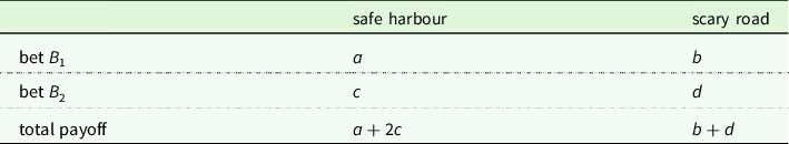
Here, $a,b,c$
and d are (possibly negative) payoffs. Hence, if the driver accepts the bet
$a,b,c$
and d are (possibly negative) payoffs. Hence, if the driver accepts the bet ${B_1}$
, then he receives a if a safe harbour is reached, and b if the scary road is reached. Similarly, if he accepts the bet
${B_1}$
, then he receives a if a safe harbour is reached, and b if the scary road is reached. Similarly, if he accepts the bet ${B_2}$
, then he receives c if a safe harbour is reached, and d if he reaches the scary road. If the payoff is negative, say
${B_2}$
, then he receives c if a safe harbour is reached, and d if he reaches the scary road. If the payoff is negative, say $ - e$
with
$ - e$
with $e \gt 0$
, then by receiving this payoff we actually mean that the driver must pay the amount e. Recall that, if a safe harbour is reached, then the bet
$e \gt 0$
, then by receiving this payoff we actually mean that the driver must pay the amount e. Recall that, if a safe harbour is reached, then the bet ${B_2}$
will be offered twice, at both exits of the highway. Hence, if you accept
${B_2}$
will be offered twice, at both exits of the highway. Hence, if you accept ${B_2}$
at both occasions, the amount c will be received twice too, resulting in a total amount of
${B_2}$
at both occasions, the amount c will be received twice too, resulting in a total amount of $2c$
. This system of bets is called a Dutch strategy if
$2c$
. This system of bets is called a Dutch strategy if $a + 2c \lt 0$
and
$a + 2c \lt 0$
and $b + d \lt 0$
. In this case, the total payoff from accepting the two bets, no matter whether you reach a safe harbour or the scary road, will always be negative.
$b + d \lt 0$
. In this case, the total payoff from accepting the two bets, no matter whether you reach a safe harbour or the scary road, will always be negative.
When will the driver be willing to accept the bets ${B_1}$
and
${B_1}$
and ${B_2}$
? Precisely when the expected payoff from accepting the bet is greater than zero. It is important that the bet
${B_2}$
? Precisely when the expected payoff from accepting the bet is greater than zero. It is important that the bet ${B_1}$
is evaluated with respect to the ex ante beliefs, whereas the driver uses his conditional beliefs to evaluate the bet
${B_1}$
is evaluated with respect to the ex ante beliefs, whereas the driver uses his conditional beliefs to evaluate the bet ${B_2}$
. Suppose that the driver, ex ante, assigns probabilities p and
${B_2}$
. Suppose that the driver, ex ante, assigns probabilities p and $1 - p$
to reaching a safe harbour and reaching the scary road, respectively. Then, his expected payoff from accepting the bet
$1 - p$
to reaching a safe harbour and reaching the scary road, respectively. Then, his expected payoff from accepting the bet ${B_1}$
would be
${B_1}$
would be
 $$EU({B_1}) = p \cdot a + (1 - p) \cdot b.$$
Assume that his conditional beliefs, upon seeing an exit on the highway, assign probabilities q and $1 - q$
to these two events. Then, the expected payoff from accepting the bet
$1 - q$
to these two events. Then, the expected payoff from accepting the bet ${B_2}$
on the highway would be
${B_2}$
on the highway would be
 $$EU({B_2}) = q \cdot c + (1 - q) \cdot d.$$
Therefore, the driver would be willing to accept the system of bets if $EU({B_1}) \gt 0$
and
$EU({B_1}) \gt 0$
and $EU({B_2}) \gt 0$
.
$EU({B_2}) \gt 0$
.
5.2. Immunity against Dutch strategies
We will now show that the driver is immune against Dutch strategies precisely when he revises his beliefs by Bayesian updating. Before doing so, we first characterize Bayesian updating in terms of the relationship between the ex ante probability p and the conditional probability q assigned to a safe harbour.
As before, let the three destinations motel, house and scary road be denoted by $A,B$
and C, respectively, and let
$A,B$
and C, respectively, and let $At1,At2,Bt1,Bt2,Ct1,Ct2$
be the centred possibilities of reaching each of these destinations, indexed by time. We have seen that seeing an exit can be identified with the event
$At1,At2,Bt1,Bt2,Ct1,Ct2$
be the centred possibilities of reaching each of these destinations, indexed by time. We have seen that seeing an exit can be identified with the event $E = \{ At1,At2,Bt1,Bt2,Ct1\} $
, where the possibility
$E = \{ At1,At2,Bt1,Bt2,Ct1\} $
, where the possibility $Ct2$
has been ruled out. If we adopt the notation from Table 3, with
$Ct2$
has been ruled out. If we adopt the notation from Table 3, with $\alpha = \beta = \gamma = {1 \over 2}$
, then the ex ante probability assigned to a safe harbour is
$\alpha = \beta = \gamma = {1 \over 2}$
, then the ex ante probability assigned to a safe harbour is
 $$p = \pi $$
whereas the conditional probability assigned to a safe harbour, obtained from Bayesian updating after seeing an exit, is
 $$q = {\pi \over {1 - {1 \over 2}(1 - \pi )}} = {{2p} \over {1 + p}}.$$
Therefore,
 $${q \over {1 - q}} = 2 \cdot {p \over {1 - p}}.$$
This relationship characterizes Bayesian updating.
The following result states that the driver will only be immune against Dutch strategies if he revises his beliefs by Bayesian updating.
Theorem 5.1. Suppose that ex ante, the driver assigns probability p and $1 - p$
to reaching a safe harbour versus reaching the scary road, and that on the highway he assigns probabilities q and
$1 - p$
to reaching a safe harbour versus reaching the scary road, and that on the highway he assigns probabilities q and $1 - q$
to these two events. Assume that both p and q are strictly between 0 and 1. Then, there is no Dutch strategy of the form above that the driver is willing to accept, if and only if,
$1 - q$
to these two events. Assume that both p and q are strictly between 0 and 1. Then, there is no Dutch strategy of the form above that the driver is willing to accept, if and only if,
 $${q \over {1 - q}} = 2 \cdot {p \over {1 - p}},$$
that is, if and only if the driver revises his beliefs by Bayesian updating.
The condition in this theorem is visualized in Figure 2, and the formal proof is given in the Appendix. The theorem thus asserts that, if we adopt the model with centred possibilities as proposed in section 4, then the solution we put forward in that section is the only plan that (a) is optimal for the driver once he sees an exit, and (b) makes him immune against Dutch strategies. Any other belief revision rule, including imaging, allows for the design of a Dutch strategy that the driver is willing to accept.
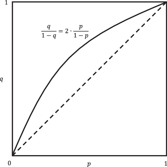
Figure 2. Immunity against Dutch strategies.
6. Related Literature
6.1. The modified multiself consistency approach
In section 2, but also at other places, we have discussed the possible tension between optimal planning and the time consistency problem in the absentminded driver problem as it has been perceived in the literature. As a possible resolution to this tension, Piccione and Rubinstein (Reference Piccione and Rubinstein1997) focus, at the end of the paper, on a different type of time consistency, called ‘modified multiself consistency’. The difference with the usual time consistency is that the driver is now modelled as a system with two agents: one who takes the decision at the first exit, and one who takes the decision at the second exit. Of course, ‘in equilibrium’, both agents must reach the same decision, as the driver cannot distinguish between the two exits. But the optimality criterion is different now: Instead of requiring that the driver cannot do better, given his beliefs, by uniformly changing his decision at both exits, it is now required that the first agent cannot do better, given his beliefs and given the fixed randomization of the second agent. Strategies that satisfy this criterion are called ‘modified multiself consistent’.
It may be verified that the ex ante optimal plan, to continue at each exit with probability ${2 \over 3}$
, is modified multiself consistent. Indeed, given the belief of being at the first exit with probability 0.6, and given the belief that the second agent will continue with probability
${2 \over 3}$
, is modified multiself consistent. Indeed, given the belief of being at the first exit with probability 0.6, and given the belief that the second agent will continue with probability ${2 \over 3}$
, the expected utilities for the first agent of continuing and leaving are both 1.6, and hence it remains optimal for the first agent to randomize.
${2 \over 3}$
, the expected utilities for the first agent of continuing and leaving are both 1.6, and hence it remains optimal for the first agent to randomize.
Whereas Piccione and Rubinstein (Reference Piccione and Rubinstein1997) do not state a clear preference for either their standard form of time consistency or modified multiself consistency, Aumann et al. (Reference Aumann, Hart and Perry1997) claim that the latter notion of consistency is the more natural one. In their paper this type of consistency is called ‘action-optimality’. They argue that if modified multiself consistency is adopted as the only reasonable time consistency criterion, then the paradox in the absentminded driver problem disappears. Indeed, as we have seen above, the unique ex ante optimal plan is also modified multiself consistent.
Also Gilboa’s (Reference Gilboa1997) analysis eventually leads to the criterion of modified multiself consistency, but via a different route. Gilboa transforms the decision tree from Figure 1 into a two-player game that satisfies perfect recall, by having nature determine at random which of the two agents will act at the first exit. The two agents act as the two players in the game, with identical utilities at the end. In particular, an agent believes that he will never have to act twice in a row, removing absentmindedness – and thereby imperfect recall – from the game. The symmetric Nash equilibria of this modified two-player game correspond precisely to the strategies in the original decision tree that are modified multiself consistent.
Note that with our approach there is no need for a modification of the optimality criterion. Indeed, we have argued that the no news assumption is not valid, and therefore the decision problems ex ante and on the highway are fundamentally different. In that light, the tension between time consistency and optimal planning ceases to be an issue within our approach.
6.2. Other approaches
As we have seen above, the ex ante optimal plan to continue with probability ${2 \over 3}$
is no longer optimal if the driver finds himself on the highway, at least if we do not view the driver as a system with two separate agents. In section 7 we argued that this should not come as a surprise, since the driver learns something substantial upon reaching an exit, which is that the state
${2 \over 3}$
is no longer optimal if the driver finds himself on the highway, at least if we do not view the driver as a system with two separate agents. In section 7 we argued that this should not come as a surprise, since the driver learns something substantial upon reaching an exit, which is that the state $C{t_2}$
is no longer possible.
$C{t_2}$
is no longer possible.
Rabinowicz (Reference Rabinowicz2003) puts forward a different argument for why the driver’s decision problem changes when reaching an exit. It argues that the driver’s doxastic state at the highway is fundamentally different from the ex ante stage, because the driver at the highway realizes that he may no longer be able to fully implement the strategy he planned at the ex ante stage. To be more precise, a strategy describes the (deterministic or probabilistic) choice the driver plans to make each time he sees an exit. However, when he is at the highway and sees an exit, he realizes this may well be the second exit already, which would mean that he is no longer able to fully implement the strategy at both exits. As, according to Rabinowicz, the driver’s mental state at the ex ante stage is fundamentally different from when he finds himself on the highway, it is argued that there is no real paradox here. Note that we have argued for a similarly ‘deflationist’ resolution of the absent-minded problem in sections 4-7, but our approach differs from Rabinowicz as it does not involve modelling the driver’s internal mental states.
Halpern and Pass (Reference Halpern and Pass2016) propose the new concept of ‘sequential equilibrium’ for dynamic games with imperfect recall. This includes the absentminded driver problem as a special case. An important ingredient of their concept is that at information sets containing consecutive nodes – like the one in the absentminded driver problem – the player’s belief should only assign positive probability to nodes that come first. In the absentminded driver example, this would mean that the driver’s belief should assign probability 1 to the first exit. Clearly then, the decision problem for the driver at his information set would be the same as at the ex ante stage, removing the tension between optimal planning and time consistency from the outset.
Finally, Schwarz (Reference Schwarz2015) investigates the absentminded driver problem by considering three different states: being at the first exit and believing that you would continue at the second exit, being at the first exit and believing that you would leave at the second exit, and being at the second exit. Hence, the driver’s counterfactual action at the second exit is included in the description of a state. Schwarz analyses the problem by using two different approaches: a causal decision theory approach (Savage Reference Savage1972; Lewis Reference Lewis1981a) and an evidential decision theory approach (Jeffrey Reference Jeffrey1990). The main difference is that in the first approach, the driver holds a fixed, subjective probabilistic belief about the three states which he then uses to determine what to do. In the evidential decision theory approach, in turn, the driver assumes that he will make the same choice at every exit, so bases his belief about the states on the action he is planning to take.
Schwarz starts by investigating the scenario where no randomization is allowed. The causal decision theory approach then leads to an ‘unstable’ decision problem where the attractiveness of a choice is inversely related to the probability assigned to that choice. In particular, there is a cut-off probability for continuing such that continuing is optimal precisely when the probability with which the driver believes to continue is below the cut-off. It is argued that some dynamics of rational deliberation à la Skyrms (Reference Skyrms1990) may lead the driver to an equilibrium state of indecision in which the probability with which he believes to continue is equal to the cut-off probability. At such a state, the driver would thus be indifferent between continuing and leaving the highway at an exit. Depending on whether a certain uniformity condition is assumed or not, the cut-off probability for continuing will be either ${2 \over 3}$
or
${2 \over 3}$
or ${4 \over 5}$
. The evidential decision theory approach, in contrast, leads to an unambiguous recommendation, which is to continue at the exit.
${4 \over 5}$
. The evidential decision theory approach, in contrast, leads to an unambiguous recommendation, which is to continue at the exit.
Subsequently, the analysis is extended to the setting where the driver is allowed to randomize between the two options ‘continue’ and ‘leave’. This is simulated by letting the driver use a biased coin at both exits. The set of states must then be enlarged, as a state must also specify which bias the driver will be using at the second exit if he is currently at the first exit. The causal decision theoretic analysis becomes analogous to the modified multiself approach in Piccione and Rubinstein (Reference Piccione and Rubinstein1997), leading to an optimal coin with bias ${2 \over 3}$
towards continuing. The evidential decision theory approach, however, comes to a different conclusion. The reason is that within this approach, the driver must believe that whatever bias he chooses, he will always use that same bias at both exits. Schwarz then shows that the optimal bias depends on the way in which the driver calculates the conditional probabilities relevant to his decision, in a way that mirrors the difference between so-called ‘thirder’ and ‘halfer’ positions in the Sleeping Beauty problem. While the solution that we have put forward in section 4 agrees with Schwarz’s combination of evidential decision theory plus the ‘thirder’ conditional probabilities, we arrive at this value through a different reasoning. In particular, in our model the states do not include counterfactual information, and our solution is not dependent on the choice of evidential decision theory.
${2 \over 3}$
towards continuing. The evidential decision theory approach, however, comes to a different conclusion. The reason is that within this approach, the driver must believe that whatever bias he chooses, he will always use that same bias at both exits. Schwarz then shows that the optimal bias depends on the way in which the driver calculates the conditional probabilities relevant to his decision, in a way that mirrors the difference between so-called ‘thirder’ and ‘halfer’ positions in the Sleeping Beauty problem. While the solution that we have put forward in section 4 agrees with Schwarz’s combination of evidential decision theory plus the ‘thirder’ conditional probabilities, we arrive at this value through a different reasoning. In particular, in our model the states do not include counterfactual information, and our solution is not dependent on the choice of evidential decision theory.
6.3. Discussion
Each of the approaches above, except Schwarz (Reference Schwarz2015) perhaps, may be viewed as an attempt to remove the tension between ex ante optimality and time consistency in the absentminded driver problem. In our view, however, there are some conceptual problems with these approaches.
Savage (Reference Savage1972) assumes, in his axiomatization of expected utility, that the decision maker cannot influence the state of the world by the act he chooses. It is precisely this act-state independence that is being violated in each of the papers above, except Gilboa (Reference Gilboa1997). Footnote 5 Indeed, in each of these papers except Schwarz (Reference Schwarz2015), if the driver finds himself on the highway, then the relevant states of the world are the events ‘I am at the first exit’ and ‘I am at the second exit’. Given the time periods reproduced in Figure 1, the first and second state can alternatively be described as ‘time period is 1’ and ‘time period is 2 and I continued at time period 1’. Clearly, whether or not the second state is realized crucially depends on which act is chosen. That is, Savage’s act-state independence is violated. In Schwarz (Reference Schwarz2015), the relevant states are extended to ‘I am at the first exit and would continue at the second exit’, ‘I am at the first exit and would leave at the second exit’, and ‘I am at the second exit’. Also here, the act chosen will influence the state that is realized, if one takes an evidential decision theory approach. In contrast, our approach in section 3 models the absentminded driver problem in a way that restores the act-state independence.
Another assumption in Savage’s framework is that the states of the world represent mutually exclusive events. However, in all of the papers above, except Gilboa (Reference Gilboa1997), the states are not mutually exclusive from an ex ante perspective. Indeed, before leaving the friend’s house, the event of reaching the second exit is perfectly compatible with – in fact, can only happen after – reaching the first exit. This fact is explicitly acknowledged by Piccione and Rubinstein when discussing their notion of consistent beliefs: When deriving the consistent belief probabilities from a given strategy, they state that the total ex ante probability of reaching the first or second exit may be larger than 1 (in fact, will be larger than 1), precisely because these two events are not mutually exclusive from an ex ante perspective. In that sense, their notion of consistency is different from standard Bayesian updating, as this only applies to mutually exclusive events. Compare this to our approaches in sections 3 and 4 where the relevant states of the world represent mutually exclusive events. As such, Bayesian updating does not need to be modified in our settings.
Piccione and Rubinstein (Reference Piccione and Rubinstein1997) introduce the notion of ‘Z-consistency’ as an alternative way of updating beliefs, and show by means of examples that it differs from consistency. They state that they are not sure which of these two notions of consistency is more appealing. This ambiguity as to which updating rule must be used is a direct consequence of the states of the world not being mutually exclusive from an ex ante perspective.
The consistency notion used by Halpern and Pass (Reference Halpern and Pass2016) is also different from the usual Bayesian updating, as they require the driver to assign probability 1 to the first exit, irrespective of his plan. However, we believe that this restriction goes against the essence of the absentminded driver problem, which is that the driver is inherently uncertain about the exit he sees, and takes this information to be relevant for what he should choose.
Finally, we see some conceptual problems with the multiself approach that is being used in each of the papers above, except Halpern and Pass (Reference Halpern and Pass2016). The main idea is that the driver is split into two separate agents, one choosing at the first exit and one at the second exit. In Gilboa (Reference Gilboa1997), these two agents are even explicitly modelled as two separate players. Moreover, if from a given plan an agent compares his planned choice with an alternative, counterfactual choice, then he assumes that the other agent will still stick to his planned choice. But how reasonable is this assumption? At the end, the two agents are time-slices of the same person, and so it is natural to think that the reasoning strategies and cognitive resources at their disposal are identical. If one arrives at a unique rational strategy, the other would also reach the same conclusion, and hence it seems likely that agent 1 could counterfactually change his choice along with agent 2.
7. Time Consistency Revisited
A common concern in the analysis of the absentminded driver problem is time consistency. As we recalled in sections 2 and 6, a recurring motivation for the solutions that have been discussed in the literature is to resolve the apparent inconsistency between the driver’s optimal strategy ex ante (before he starts the journey) and when he reaches an exit. This poses a problem because it is implicitly assumed that the driver does not learn anything new between these times – call this the no news assumption. He always knew that he was going to reach an exit, and he should not be surprised when he does. Therefore, the driver should not update his beliefs upon reaching an exit, and the discrepancy between his optimal strategies when considered ex ante vs. when reaching an exit (what we will call interim) cannot be explained by a change in the probabilities assigned to the relevant states of the world. Starting from the no news assumption, most of the solutions in the literature (see section 6) attempt to resolve the issue of time inconsistency by looking for a strategy that could be characterized as rational, according to some modified notion of optimality, both ex ante and interim.
Contrary to this received approach, our analysis highlights that the no news assumption is incorrect. The driver learns some new relevant information upon arriving at an exit, namely that $Ct2$
is not the case at this point. Since this is a possibility that the driver eliminates when he reaches an exit, he should update on this information. Failing to do so, moreover, would lead to diachronic inconsistency and vulnerability to a Dutch strategy. Therefore, the driver’s beliefs ex ante and upon reaching an exit differ, but are not time inconsistent. On the contrary, the difference results from applying standard Bayesian updating upon learning a new piece of evidence. Our analysis explains why the driver’s changing beliefs, and the resulting change in optimal strategies, are in fact time consistent, eliminating the need to resolve the apparent discrepancy that motivated previous solutions presented in the literature.
$Ct2$
is not the case at this point. Since this is a possibility that the driver eliminates when he reaches an exit, he should update on this information. Failing to do so, moreover, would lead to diachronic inconsistency and vulnerability to a Dutch strategy. Therefore, the driver’s beliefs ex ante and upon reaching an exit differ, but are not time inconsistent. On the contrary, the difference results from applying standard Bayesian updating upon learning a new piece of evidence. Our analysis explains why the driver’s changing beliefs, and the resulting change in optimal strategies, are in fact time consistent, eliminating the need to resolve the apparent discrepancy that motivated previous solutions presented in the literature.
Still, one may pose the following objection to our analysis, based on the idea of forming a commitment. Suppose that the driver has the possibility, ex ante, of forming a commitment, that is, selecting a strategy that will be binding for him whenever he reaches an exit. Based on our analysis, the optimal strategy for the driver ex ante would be to continue with a probability of ${2 \over 3}$
. However, if he were to commit to this strategy, he would regret doing so at the moment he reaches an exit, when the optimal strategy after updating would be to continue with probability 0.53. Under these conditions, would it be rational for the driver to choose to commit to the ex ante optimal strategy? Or should he commit to the strategy he knows will be optimal for him after updating, even though it is not optimal at the time he makes the commitment?
${2 \over 3}$
. However, if he were to commit to this strategy, he would regret doing so at the moment he reaches an exit, when the optimal strategy after updating would be to continue with probability 0.53. Under these conditions, would it be rational for the driver to choose to commit to the ex ante optimal strategy? Or should he commit to the strategy he knows will be optimal for him after updating, even though it is not optimal at the time he makes the commitment?
Neither option seems rational. If the driver commits to the ex ante optimal strategy, he will come to regret it, based on his own beliefs at the time when he needs to implement the strategy. Choosing to commit to the other strategy, on the other hand, would be irrational from the ex ante perspective. Thus, if the driver has the option to commit, it seems that neither of the available strategies (the ex ante optimal one or the interim optimal one) are rational to commit to.
For a rational agent who plans to update her beliefs via conditioning, and does not expect to forget any of her experiences, forming a commitment is redundant, since her present and future (expected) optimal strategies are identical (see, for instance, Perea Reference Perea2012, Lemma 8.14.9). However, if the agent expects her future self to become irrational, then it may be rational to form a commitment now in order to prevent herself from making a bad choice in the future, as in the story of Ulysses tying himself to the mast of his ship in order to escape the sirens’ call (van Fraassen Reference van Fraassen1995). Thus, forming a commitment in the face of an expected deviation, in the future, from what is the present optimal strategy, may be rational if the agent expects to become irrational by the time of making a decision.
Interestingly, the case of absentmindedness illustrates how forming a commitment is not always either redundant or necessary to prevent anticipated irrationality. Sometimes, it is simply not possible to rationally commit. Although his future beliefs deviate predictably from his ex ante beliefs, the driver’s future self is not irrational. Upon reaching an exit, the driver arrives at the new beliefs by conditioning on newly acquired evidence, as we have seen in section 4, and committing to the ex ante optimal strategy would make him vulnerable to a Dutch Strategy, as we have shown in section 5. So, although the driver expects that he will deviate from his ex ante optimal strategy when he will make a decision in the future, he can’t justify committing to the ex ante optimal strategy on the basis of his own future irrationality.
Absentmindedness means that the future driver cannot locate himself in time. When he approaches an exit, he is uncertain whether it is the first or the second one. This happens predictably and therefore his evidence at any time that he approaches an exit is the same. But this also means that when he considers, ex ante, what his own beliefs will be later during the journey, on the highway, he is not referring to his future self at a definite point in time. Later here refers both to his future self approaching the first exit, and his future self approaching the second exit (if he gets that far). Footnote 6 If the driver were expected to defer to his rational, future self, this would raise the question: to his future self at which point in time?
Ex ante, the driver can only be certain that he will hit the first exit (since that exit is reached no matter what the final destination), at which point he will update his beliefs and optimal strategy in the way that we have described. So, a natural answer to the previous question is to defer to the driver’s future self at the only time he is certain to reach an exit, that is $t1$
. Interpreted in this way, later picks out
$t1$
. Interpreted in this way, later picks out $t1$
, but it is not a stopping time (Schervish et al., Reference Schervish, Seidenfeld and Kadane2004). A (possibly random) time T is called a stopping time when, at any point in time, the agent knows whether T has already occurred or not. An example of a stopping time would be the day of your son’s first birthday (assuming that you do not forget what day it is!), or the first time a coin that you are about to toss repeatedly comes up heads, assuming that you observe and don’t forget any of the previous tosses. Since the driver does not know he has reached the first exit when he is there,
$t1$
, but it is not a stopping time (Schervish et al., Reference Schervish, Seidenfeld and Kadane2004). A (possibly random) time T is called a stopping time when, at any point in time, the agent knows whether T has already occurred or not. An example of a stopping time would be the day of your son’s first birthday (assuming that you do not forget what day it is!), or the first time a coin that you are about to toss repeatedly comes up heads, assuming that you observe and don’t forget any of the previous tosses. Since the driver does not know he has reached the first exit when he is there, ${t_1}$
is not a stopping time in our case. Moreover, learning that later, so interpreted, has arrived would give the driver information that changes his optimal strategy: if he knew that he was approaching the first exit, then it would be optimal for him to continue.
${t_1}$
is not a stopping time in our case. Moreover, learning that later, so interpreted, has arrived would give the driver information that changes his optimal strategy: if he knew that he was approaching the first exit, then it would be optimal for him to continue.
Under these conditions (that is, later not being a stopping time, and the additional information that later has arrived being relevant to the driver’s other beliefs), Schervish et al. (Reference Schervish, Seidenfeld and Kadane2004) show that the so-called Principle of Reflection does not apply.
Footnote 7
This principle, introduced by van Fraassen (Reference van Fraassen1984), says that for any two times ${t_1} \lt {t_2}$
, and for any event A, your credence in A at
${t_1} \lt {t_2}$
, and for any event A, your credence in A at ${t_1}$
, conditional on your credence in A at
${t_1}$
, conditional on your credence in A at ${t_2}$
being r, should also be r. That is:
${t_2}$
being r, should also be r. That is: ${P_{{t_1}}}(A|{P_{{t_2}}}(A) = r) = r$
. Since Reflection does not apply to our case, the absent-minded driver’s ex ante beliefs do not reflect his expected later beliefs (Schervish et al., Reference Schervish, Seidenfeld and Kadane2004). Therefore, he cannot rationally commit ex ante to a strategy that is optimal later, since his own beliefs ex ante should not rationally reflect the beliefs he will have later.
${P_{{t_1}}}(A|{P_{{t_2}}}(A) = r) = r$
. Since Reflection does not apply to our case, the absent-minded driver’s ex ante beliefs do not reflect his expected later beliefs (Schervish et al., Reference Schervish, Seidenfeld and Kadane2004). Therefore, he cannot rationally commit ex ante to a strategy that is optimal later, since his own beliefs ex ante should not rationally reflect the beliefs he will have later.
Anticipating his own absentmindedness, the driver can only make rational decisions at the moment when it is required. If he is required to pick a strategy ex ante, and prevented from changing it along the way, then he should pick the ex ante optimal strategy, which differs from what he would choose on the highway. In this scenario, the driver is effectively occupying the role of a passenger, since he has no control over the direction travelled by the car during the journey. If, instead, the driver is allowed to make choices while on the highway, then he should opt for the interim optimal strategy, deviating from the choice probability that he would have picked ex ante. This is not a sign of dynamic inconsistency, since the change in beliefs is the result of rational updating, and commitment is not appropriate in this case.
8. Conclusion
The absentminded driver problem presents a decision situation that challenges standard approaches to modelling one-person decision problems. First, act-state independence, a core assumption of the Savage (Reference Savage1972) framework, is violated. Second, the decision problem appears unstable, since the optimal choice appears to change if we consider it from an ex ante perspective, or at the moment of choice, resulting in time inconsistency.
We have presented two new approaches to the resolution of the absentminded driver problem that address these two issues. In the first proposal, we present a version of the absentminded driver problem where we model the driver as being uncertain about his own degree of absentmindedness. This approach is completely in line with Savage’s framework, and the resulting solution satisfies both act-state independence and time consistency.
In the second proposal, we model states as centred possibilities. This allows us to model explicitly the driver’s uncertainty regarding both the destination that he will eventually reach, and the time period at which he is located. Using this model, we derive the optimal choice probability of continuing for the driver, taking into account the centred evidence that is available to him at the time he makes a choice. We show that Bayesian conditioning in this setting is the only updating strategy that prevents vulnerability to a sure loss via a Dutch strategy.
A surprising implication of our second approach is that it highlights how commitment is sometimes impossible, since the driver’s ex ante and interim optimal strategies differ predictably but rationally. We have argued that this conclusion does not violate time consistency, because it is based on updating on new evidence. Our discussion of time consistency in the setting of absentmindedness has also highlighted the relationship between planning, commitment and van Fraassen’s Reflection principle. Ex ante planning is not possible, because commitment to any strategy but the one that is optimal at the time of making a choice is not appropriate in similar cases, for wholly anticipated and yet rational reasons.
Acknowledgements
We would like to thank Johanna Thoma and Wolfgang Schwarz for helpful feedback, two anonymous reviewers at Economics and Philosophy and three anonymous referees at the TARK XVIII conference for their useful comments. Special gratitude goes to Teddy Seidenfeld for extensive and helpful discussions.
Silvia Milano is a Lecturer in Philosophy at the University of Exeter, Department of Social and Political Sciences, Philosophy and Anthropology, and the Egenis Centre for the Study of Life Sciences. She obtained her PhD from the London School of Economics and Political Science with a thesis on ‘De se beliefs and centred uncertainty’. Her article ‘Bayesian Beauty’ was awarded the 2017/18 LSE Philosophy Popper prize. URL: https://www.silvia-milano.com/.
Andrés Perea is an Associate Professor at Maastricht University, Department of Quantitative Economics. His research focuses on the foundations of game theory and decision theory, with a special focus on epistemic game theory. Recent publications: ‘Common belief in rationality in games with unawareness’, (2022) Mathematical Social Sciences 119, 11-30; ‘Common belief in rationality in psychological games: belief-dependent utility and the limits of strategic reasoning’ (2022) (with Stephan Jagau), Journal of Mathematical Economics 100, https://doi.org/10.1016/j.jmateco.2022.102635; ‘Incomplete information and iterated strict dominance’ (2021) (with Christian Bach), Oxford Economic Papers 73, 820–836. URL: https://www.epicenter.name/Perea/.
Appendix
Proof of Theorem 5.1.
We first show that, if ${q \over {1 - q}} = 2 \cdot {p \over {1 - p}}$
, then the driver will never accept a Dutch strategy. To see this, suppose that the driver would be willing to accept the bets
${q \over {1 - q}} = 2 \cdot {p \over {1 - p}}$
, then the driver will never accept a Dutch strategy. To see this, suppose that the driver would be willing to accept the bets ${B_1}$
and
${B_1}$
and ${B_2}$
. Then,
${B_2}$
. Then, $EU({B_2}) \gt 0$
and hence
$EU({B_2}) \gt 0$
and hence
 $$q \cdot c + (1 - q) \cdot d \gt 0.$$
Dividing by $1 - q$
thus yields
$1 - q$
thus yields
 $${q \over {1 - q}} \cdot c + d \gt 0.$$
As ${q \over {1 - q}} = 2 \cdot {p \over {1 - p}}$
, we obtain
${q \over {1 - q}} = 2 \cdot {p \over {1 - p}}$
, we obtain
 $${p \over {1 - p}} \cdot 2c + d \gt 0,$$
and hence
 $$p \cdot 2c + (1 - p) \cdot d \gt 0.$$
Moreover, as the driver is willing to accept the bet ${B_1}$
, it must be that
${B_1}$
, it must be that $EU({B_1}) \gt 0$
, which means
$EU({B_1}) \gt 0$
, which means
 $$p \cdot a + (1 - p) \cdot b \gt 0.$$
By adding up the last two inequalities we get
 $$p \cdot (a + 2c) + (1 - p) \cdot (b + d) \gt 0,$$
which implies that either $a + 2c \gt 0$
or
$a + 2c \gt 0$
or $b + d \gt 0$
. Thus, the system of bets that the driver is willing to accept cannot be a Dutch strategy.
$b + d \gt 0$
. Thus, the system of bets that the driver is willing to accept cannot be a Dutch strategy.
Next, assume that the condition in the theorem is violated, that is, ${q \over {1 - q}} \ne 2 \cdot {p \over {1 - p}}$
. We will distinguish two cases: (1)
${q \over {1 - q}} \ne 2 \cdot {p \over {1 - p}}$
. We will distinguish two cases: (1) ${q \over {1 - q}} \lt 2 \cdot {p \over {1 - p}}$
, and (2)
${q \over {1 - q}} \lt 2 \cdot {p \over {1 - p}}$
, and (2) ${q \over {1 - q}} \gt 2 \cdot {p \over {1 - p}}$
. For both cases we will construct a Dutch strategy that the driver is willing to accept.
${q \over {1 - q}} \gt 2 \cdot {p \over {1 - p}}$
. For both cases we will construct a Dutch strategy that the driver is willing to accept.
Case 1. Assume that ${q \over {1 - q}} \lt 2 \cdot {p \over {1 - p}}$
.
${q \over {1 - q}} \lt 2 \cdot {p \over {1 - p}}$
.
Define the number
 $$\varepsilon : = {{2p/(1 - p)} \over {q/(1 - q)}} - 1,$$
which is positive. Let the payoffs of the bets ${B_1}$
and
${B_1}$
and ${B_2}$
in Table 4 be given by
${B_2}$
in Table 4 be given by
 $$a: = 2,\;\;\;{\kern 1pt} b: = - \left(1 + {3 \over 4}\varepsilon \right) \cdot {q \over {1 - q}},\;\;\;{\kern 1pt} c: = - 1 - {1 \over 4}\varepsilon ,\;\;\;{\kern 1pt} d: = \left(1 + {1 \over 2}\varepsilon \right) \cdot {q \over {1 - q}}.$$
We show that this system of bets is a Dutch book that the driver is willing to accept. First, it may be verified that $a + 2c \lt 0$
and
$a + 2c \lt 0$
and $b + d \lt 0$
, and therefore this is a Dutch strategy. Moreover,
$b + d \lt 0$
, and therefore this is a Dutch strategy. Moreover,
 $$EU({B_1}) = p \cdot 2 - (1 - p) \cdot \left(1 + {3 \over 4}\varepsilon \right) \cdot {q \over {1 - q}}$$
 $$ \hskip +18pt {\gt p \cdot 2 - (1 - p) \cdot (1 + \varepsilon ) \cdot {q \over {1 - q}}}$$
 $$ = p \cdot 2 - (1 - p) \cdot 2 \cdot {p \over {1 - p}}$$
 $$ \hskip -35pt= p \cdot 2 - p \cdot 2 = 0.$$
In the second equality we have used the definition of $\varepsilon $
. Thus, the driver is willing to accept
$\varepsilon $
. Thus, the driver is willing to accept ${B_1}$
. Also,
${B_1}$
. Also,
 $$\displaylines{ EU({B_2}) = - q \cdot \left(1 + {1 \over 4}\varepsilon \right) + (1 - q) \cdot \left(1 + {1 \over 2}\varepsilon \right) \cdot {q \over {1 - q}} \cr = - q \cdot \left(1 + {1 \over 4}\varepsilon \right) + q \cdot \left(1 + {1 \over 2}\varepsilon \right) \gt 0, \cr} $$
which means that the driver is also willing to accept ${B_2}$
. Summarizing, we see that there is a Dutch strategy that the driver is willing to accept.
${B_2}$
. Summarizing, we see that there is a Dutch strategy that the driver is willing to accept.
Case 2. Suppose that ${q \over {1 - q}} \gt 2 \cdot {p \over {1 - p}}$
.
${q \over {1 - q}} \gt 2 \cdot {p \over {1 - p}}$
.
Define the number
 $$\varepsilon : = 1 - {{2p/(1 - p)} \over {q/(1 - q)}},$$
which is positive. Set the payoffs of the bets ${B_1}$
and
${B_1}$
and ${B_2}$
in Table 4 by
${B_2}$
in Table 4 by
 $$a: = - 2,\;\;\;{\kern 1pt} b: = \left(1 - {3 \over 4}\varepsilon \right) \cdot {q \over {1 - q}},\;\;\;{\kern 1pt} c: = 1 - {1 \over 4}\varepsilon ,\;\;\;{\kern 1pt} d: = \left( - 1 + {1 \over 2}\varepsilon \right) \cdot {q \over {1 - q}}.$$
Like in Case 1, we show that this system of bets is a Dutch strategy that the driver is willing to accept. First, it holds that $a + 2c \lt 0$
and
$a + 2c \lt 0$
and $b + d \lt 0$
, and therefore this is a Dutch strategy. Also,
$b + d \lt 0$
, and therefore this is a Dutch strategy. Also,
 $$EU({B_1}) = - p \cdot 2 + (1 - p) \cdot \left(1 - {3 \over 4}\varepsilon \right) \cdot {q \over {1 - q}}$$
 $$ \hskip +18pt {\gt - p \cdot 2 + (1 - p) \cdot (1 - \varepsilon ) \cdot {q \over {1 - q}}}$$
 $$ \hskip -7pt {= - p \cdot 2 + (1 - p) \cdot 2 \cdot {p \over {1 - p}}}$$
 $$ \hskip -37pt {= - p \cdot 2 + p \cdot 2 = 0}.$$
In the second equality we have used the definition of $\varepsilon $
. Hence, the driver is willing to accept
$\varepsilon $
. Hence, the driver is willing to accept ${B_1}$
. Moreover,
${B_1}$
. Moreover,
 $$\displaylines{ EU({B_2}) = q \cdot \left(1 - {1 \over 4}\varepsilon \right) + (1 - q) \cdot \left( - 1 + {1 \over 2}\varepsilon \right) \cdot {q \over {1 - q}} \cr = q \cdot \left(1 - {1 \over 4}\varepsilon \right) + q \cdot \left( - 1 + {1 \over 2}\varepsilon \right) \gt 0, \cr} $$
which means that the driver is also willing to accept ${B_2}$
. Hence also in Case 2 we see that there is a Dutch strategy that the driver is willing to accept.
${B_2}$
. Hence also in Case 2 we see that there is a Dutch strategy that the driver is willing to accept.
By combining Cases 1 and 2 we conclude that, whenever ${q \over {1 - q}} \ne 2 \cdot {p \over {1 - p}}$
, we can always construct a Dutch strategy that the driver is willing to accept.
${q \over {1 - q}} \ne 2 \cdot {p \over {1 - p}}$
, we can always construct a Dutch strategy that the driver is willing to accept.


 Open access