


Impact Statement
This perspective paper reviews the evolution and growth of machine learning (ML) models in environmental science. The opaque nature of ML models led to decades of slow growth, but exponential growth commenced around the mid-2010s. Novel ML models which have contributed to this exponential growth (e.g., deep convolutional neural networks, encoder–decoder networks, and generative-adversarial networks) are reviewed, as well as approaches to merging ML models with physics-based models.
1. Introduction
Thirty years ago, a typical environmental scientist would know some statistics but would not have heard of “machine learning” (ML) and would know artificial intelligence (AI) only through science fiction. After World War II, the great popularity of AI in science fiction led to very unrealistic expectations on how fast AI research would progress. The inevitable disappointment led to negative reviews and two major “AI winters,” periods of poor funding around 1974–1980 and 1987–1993 (Crevier, Reference Crevier1993; Nilsson, Reference Nilsson2009). Partly to focus on a more specific aspect and partly to avoid the stigma associated with AI, many researchers started to refer to their work using other names, for example, ML, where the goal of ML is to have computers learn from data without being explicitly programmed.
While there is overlap between the data methods developed in statistics and in the younger field of ML (Figure 1), ML germinated mainly in computer science, psychology, engineering, and commerce, while statistics had largely been rooted in mathematics, leading to two fairly distinct cultures (Breiman, Reference Breiman2001b). When fitting a curve to a dataset, a statistician would ensure the number of adjustable model parameters is small compared to the sample size (i.e., number of observations) to avoid overfitting (i.e., the model fitting to the noise in the data). This prudent practice in statistics is not strictly followed in ML, as the number of parameters (called “weights” in ML) can be greater, sometimes much greater, than the sample size (Krizhevsky et al., Reference Krizhevsky, Sutskever and Hinton2012), as ML has developed ways to avoid overfitting while using a large number of parameters. The relatively large number of parameters renders ML models much more difficult to interpret than statistical models; hence, ML models are often regarded somewhat dismissively as “black boxes.” In ML, the artificial neural network (NN) model called the multilayer perceptron (MLP; Rumelhart et al., Reference Rumelhart, Hinton, Williams, Rumelhart and McClelland1986; Goodfellow et al., Reference Goodfellow, Bengio and Courville2016) has become widely used since the late 1980s.
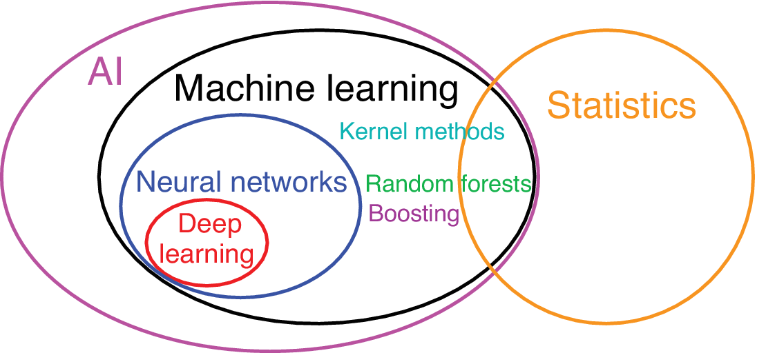
Figure 1. Venn diagram illustrating the relation between artificial intelligence, statistics, machine learning, neural networks, and deep learning, as well as kernel methods, random forests, and boosting.
How readily an environmental science (ES) adopted NN or other ML models depended on whether successful physics-based models were available. Meteorology, where dynamical models have been routinely used for weather forecasting, has been slower to embrace NN models than hydrology, where by year 2000 there were already 43 hydrological papers using NN models (Maier and Dandy, Reference Maier and Dandy2000), as physics-based models were not very skillful in forecasting streamflow from precipitation data.
Relative to linear statistical models, the nonlinear ML models also need relatively large sample size to excel. Hence, oceanography, a field with far fewer in situ observations than hydrology or meteorology, and climate science, where the longtime scales preclude large effective sample size, are fields where the application of ML models has been hampered. Furthermore, averaging daily data to produce climate data linearizes the relation between the predictors and the response variables due to the central limit theorem, thereby reducing the nonlinear modelling advantage of ML models (Yuval and Hsieh, Reference Yuval and Hsieh2002). Another disadvantage of many ML models (e.g., NN) relative to linear statistical models is that they can extrapolate much worse when given new predictor data lying outside the original training domain (Hsieh, Reference Hsieh2020), as nonlinear extrapolation is an ill-posed problem. This is not ML-specific, since any nonlinear statistical model faces the same ill-posed problem when used for extrapolation.
Overall, around year 2010, ML models were fairly well accepted in hydrology and remote sensing, but remained fringe in meteorology and even less developed in oceanography and climate science. Nevertheless, a number of books were written on the application of ML methods to ES in this earlier development phase (Abrahart et al., Reference Abrahart, Kneale and See2004; Blackwell and Chen, Reference Blackwell and Chen2009; Haupt et al., Reference Haupt, Pasini and Marzban2009; Hsieh, Reference Hsieh2009; Krasnopolsky, Reference Krasnopolsky2013). After this relatively flat phase, rapid growth of ML in ES commenced in the mid-2010s.
Section 2 looks at the emergence of new and more powerful ML methods in the last decade, whereas Section 3 reviews their applications to ES. The merging of ML and physical/dynamical models is examined in Section 4.
2. Evolution of ML Methods
The MLP NN model maps the input variables through layers of hidden neurons/nodes (i.e., intermediate variables) to the output variables. Given some training data for the input and output variables, the model weights can be solved by minimizing an objective function using a back-propagation algorithm. The traditional MLP NN is mostly limited to one or two hidden layers, because the gradients (error signals) in the back-propagation algorithm become vanishingly small after propagating through many layers. Without a solution for the vanishing gradient problem, NN research stalled while newer methods—kernel methods (e.g., support vector machines (Cortes and Vapnik, Reference Cortes and Vapnik1995)) emerging from the mid-1990s and random forests from 2001 (Breiman, Reference Breiman2001a)—seriously challenged NN’s dominant position in ML.
The traditional MLP NN has each neuron in one layer connected to all the neurons in the preceding layer. When working with image data, the MLP uses a huge number of weights—for example, mapping an input 100 × 100 image to just one neuron in the first hidden layer requires 10,000 weights! Since, in nature, biological neurons are connected only to neighboring neurons, to have every neuron in one layer of an NN model connected to all the neurons in the preceding layer is unnatural and very wasteful of computing resources. With inspiration from the animal visual cortex, the convolutional layer has been developed, where a neuron is only connected to a small patch of neurons in the preceding layer, thereby resulting in a drastic reduction of weights compared to the traditional fully connected layers and giving rise to convolutional neural networks (CNNs; LeCun et al., Reference LeCun, Boser, Denker, Henderson, Howard, Hubbard and Jackel1989).
Eventually, the vanishing gradient problem was overcome, and deep NN or deep learning (DL) models, that is, NN having $ \gtrsim 5 $
layers of mapping functions with adjustable weights (LeCun et al., Reference LeCun, Bengio and Hinton2015), emerged. In 2012, a deep NN model won the ImageNet Large Scale Visual Recognition Challenge (Krizhevsky et al., Reference Krizhevsky, Sutskever and Hinton2012). The huge reduction in the number of weights in convolutional layers made deep NN feasible.
$ \gtrsim 5 $
layers of mapping functions with adjustable weights (LeCun et al., Reference LeCun, Bengio and Hinton2015), emerged. In 2012, a deep NN model won the ImageNet Large Scale Visual Recognition Challenge (Krizhevsky et al., Reference Krizhevsky, Sutskever and Hinton2012). The huge reduction in the number of weights in convolutional layers made deep NN feasible.
With all the impressive breakthroughs in DL since 2012 (Goodfellow et al., Reference Goodfellow, Bengio and Courville2016), there is a popular misconception that DL models are superior to all other ML models. Actually, the best ML model is very problem-dependent. There are two main types of datasets, structured and unstructured. Structured datasets have a tabular format, for example, like an Excel spreadsheet, with the variables listed in columns. In contrast, unstructured datasets include images, videos, audio, text, and so forth. For unstructured datasets, DL has indeed been dominant. For structured datasets, however, ML models with shallow depth structure, for example, gradient boosting models such as XGBoost (Chen and Guestrin, Reference Chen and Guestrin2016), have often beaten deep NN in competitions, for example, those organized by Kaggle (www.kaggle.com).
How can “shallow” gradient boosting beat deep NN in structured data? Typically, in a structured dataset, the predictors are quite inhomogeneous (e.g., pressure, temperature, and humidity), whereas in an unstructured dataset, the predictors are more homogeneous (e.g., temperature at various pixels in a satellite image or at various grid points in a numerical model). Boosting is based on decision trees, where the effects of the predictors
X
are treated independently of each other, as the path through a decision tree is controlled by questions like: is “ $ {x}_1>a? $
,” “
$ {x}_1>a? $
,” “ $ {x}_2>b? $
,” and so forth (Breiman et al., Reference Breiman, Friedman, Olshen and Stone1984). In contrast, in NN, the predictors are combined by a linear combination (
$ {x}_2>b? $
,” and so forth (Breiman et al., Reference Breiman, Friedman, Olshen and Stone1984). In contrast, in NN, the predictors are combined by a linear combination ( $ {\sum}_i{w}_i{x}_i $
) before being passed through an activation/transfer function onto the next layer. With inhomogeneous predictors, for example, temperature and pressure, treating the two separately as in decision trees intuitively makes more sense than trying to add the two together by a linear combination.
$ {\sum}_i{w}_i{x}_i $
) before being passed through an activation/transfer function onto the next layer. With inhomogeneous predictors, for example, temperature and pressure, treating the two separately as in decision trees intuitively makes more sense than trying to add the two together by a linear combination.
Another type of NN architecture is the encoder–decoder model, where the encoder part first maps from a high-dimensional input space to a low-dimensional space, then the decoder part maps back to a high-dimensional output space (Figure 2). If the target output data are the same as the input data, the model becomes an autoencoder, which has been used for nonlinear principal component analysis (PCA), as the low-dimensional space can be interpreted as nonlinear principal components (Kramer, Reference Kramer1991; Monahan, Reference Monahan2000; Hsieh, Reference Hsieh2001). The popular U-net (Ronneberger et al., Reference Ronneberger, Fischer and Brox2015) is a deep CNN model with an encoder–decoder architecture.

Figure 2. The encoder–decoder is an NN model with the first part (the encoder) mapping from the input x to u, the “code” or bottleneck, and the second part (the decoder) mapping from u to the output y. Dimensional compression is achieved by forcing the signal through the bottleneck. The encoder and the decoder are each illustrated with only one hidden layer for simplicity.
In many games, having two individuals playing against each other enhances the skill level of both, for example, a soccer goal scorer practicing against a goal keeper. The generative adversarial network (GAN) has two submodels, the generator and the discriminator, playing as adversaries, with the goal of producing realistic fake data (Goodfellow et al., Reference Goodfellow, Pouget-Abadie, Mirza, Xu, Warde-Farley, Ozair, Courville and Bengio2014). Given a random input vector, the generator outputs a set of fake data. The discriminator receives either real data or fake data as input and classifies them as either “real” or “fake” (Figure 3). If a fake is correctly classified, the generator’s model weights are updated, whereas if the fake is mistaken to be real, the discriminator’s model weights are updated. The skill levels of both players improve until at the end the discriminator can only identify fake data from the generator about 50% of the time. After training is done, the discriminator is discarded while the generator is retained to produce new fake data. The variational autoencoder model provides an alternative to GAN (Kingma and Welling, Reference Kingma and Welling2014).
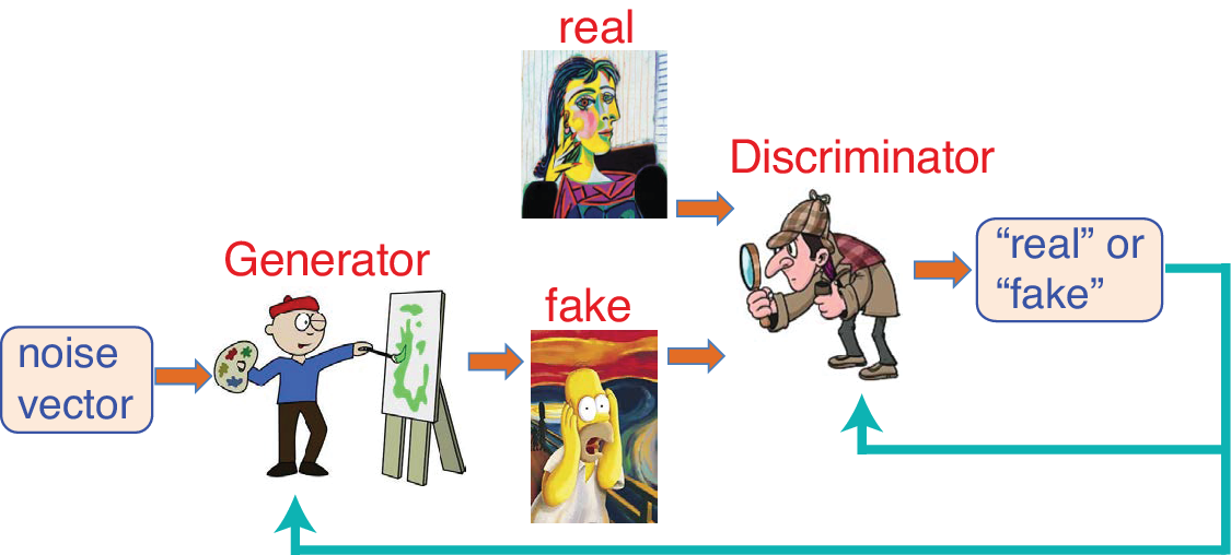
Figure 3. Generative adversarial network with the generator creating a fake image (e.g., a fake Picasso painting) from random noise input, and the discriminator classifying images as either real or fake. Whether the discriminator classifies a fake image rightly or wrongly leads, respectively, to further training for the generator or for the discriminator.
Conditional generative adversarial network (CGAN), introduced by Mirza and Osindero (Reference Mirza and Osindero2014), supplies additional input x to both the generator and the discriminator. If X is an image, CGAN can be used for image-to-image translation tasks (Isola et al., Reference Isola, Zhu, Zhou and Efros2017), for example, translating a line drawing to a photo image, a map to a satellite map, or vice versa (Figure 4).
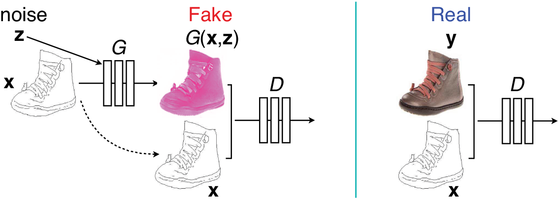
Figure 4. Conditional generative adversarial network where the generator G receives an image x and a random noise vector z as input. The discriminator D receives x plus either a fake image from G (left) or a real image y (right) as input. Here, a line drawing is converted to a photo image; similarly, a photo image can be converted to a line drawing.
Adapted from Figure 2 of Isola et al. (Reference Isola, Zhu, Zhou and Efros2017).
3. Applications in Environmental Science
Applications of ML to ES have come in roughly two groups. In the first group, ML methods are used largely as nonlinear generalizations of traditional statistical methods. For instance, MLP NN models are used for nonlinear regression, classification, PCA, and so forth (Hsieh, Reference Hsieh2009). In the second group, the ML methods do not have counterparts in statistics, for example, GAN or CGAN.
CNN models have appeared in ES in the last few years, for example, to estimate the posterior probability of three types of extreme events (tropical cyclones, atmospheric rivers, and weather fronts) from 2D images of atmospheric variables (Liu et al., Reference Liu, Racah, Prabhat, Correa, Khosrowshahi, Lavers, Kunkel, Wehner and Collins2016), to detect synoptic-scale weather fronts (cold front, warm front, and no front; Lagerquist et al., Reference Lagerquist, Mcgovern and Gagne2019) and for next-hour tornado prediction from radar images (Lagerquist et al., Reference Lagerquist, McGovern, Homeyer, Gagne and Smith2020).
Performing classification on each pixel of an image is called semantic segmentation in ML. Most CNN models for semantic segmentation use an encoder–decoder architecture, including the popular U-net deep CNN model (Ronneberger et al., Reference Ronneberger, Fischer and Brox2015), giving classification (or regression) on individual output pixels. U-net has been applied to rain-type classification (no-rain, stratiform, convective, and others) using microwave satellite images (Choi and Kim, Reference Choi and Kim2020), to precipitation estimation using satellite infrared images (Sadeghi et al., Reference Sadeghi, Phu, Hsu and Sorooshian2020) and to cloud cover nowcasting using visible and infrared images (Berthomier et al., Reference Berthomier, Pradel and Perez2020).
As traditional MLP NN models require a very large number of weights when working with 2D images or 3D spatial fields, limited sample size often necessitates the compression of input variables to a modest number of principal components by PCA, a linear technique (Jolliffe, Reference Jolliffe2002). The introduction of the CNN model has drastically reduced the number of weights, so compression by PCA is not needed, and deep CNN models have noticeably improved the performance of ML methods when working with 2D or 3D spatial fields in ES since the mid-2010s.
PCA has been used to impute missing values in datasets (Jolliffe, Reference Jolliffe2002, Section 13.6) and U-net, with its encoder–decoder architecture, can replace PCA in this task. Using sea surface temperature (SST) data from two sources (NOAA Twentieth-Century Reanalysis [20CR] and Coupled Model Intercomparison Project Phase 5 [CMIP5]), Kadow et al. (Reference Kadow, Hall and Ulbrich2020) trained U-net models, which outperformed PCA and kriging methods in imputing missing SST values.
The CGAN (Figure 4) has also been used in ES: In atmospheric remote sensing, CGAN generated cloud structures in a 2D vertical plane in the satellite’s along-track direction (Leinonen et al., Reference Leinonen, Guillaume and Yuan2019). As an alternative to U-net in super-resolution applications, CGAN has been used to convert low-resolution unmanned aircraft system images to high-resolution images (Pashaei et al., Reference Pashaei, Starek, Kamangir and Berryhill2020).
The application of ML methods to climate problems has been impeded by the relatively small effective sample size in observational records. In transfer learning, ML models trained on a dataset with large sample size can transfer their learning to a different problem hampered by a relatively small sample size. Using a CNN to learn the El Niño-Southern Oscillation (ENSO) behavior from the dynamical models (CMIP5 climate model data for 2,961 months), then transferring the learning to observed data (by further training with 103 months of reanalysis data), Ham et al. (Reference Ham, Kim and Luo2019) developed a CNN model with better accuracy in ENSO prediction than the dynamical models.
4. Merging of Machine Learning and Physics
As some components of a physical model can be computationally expensive, ML methods have been developed to substitute for the physics: For atmospheric radiation in atmospheric general circulation models (GCMs), MLP NN models have been used to replace the equations of physics (Chevallier et al., Reference Chevallier, Morcrette, Cheruy and Scott2000; Krasnopolsky et al., Reference Krasnopolsky, Fox-Rabinovitz and Belochitski2008). For a simple coupled atmosphere–ocean model of the tropical Pacific, the atmospheric component has been replaced by an NN model (Tang and Hsieh, Reference Tang and Hsieh2002). Resolving clouds in a GCM would require high spatial resolution and prohibitive costs; hence, NN models, trained by a cloud-resolving model, have been used to supply convection parametrization in a GCM (Krasnopolsky et al., Reference Krasnopolsky, Fox-Rabinovitz and Belochitski2013; Brenowitz and Bretherton, Reference Brenowitz and Bretherton2018; Rasp et al., Reference Rasp, Pritchard and Gentine2018). Increasingly, ML methods are used to learn from high-resolution numerical models, then implemented as inexpensive parametrization schemes in GCMs.
In physics-informed machine learning, ML models can be solved satisfying the laws of physics, for example, conservation of energy, mass, and so forth. In the soft constraint approach, the physics constraints are satisfied approximately by adding an extra regularization term in the objective function of an NN model (Karniadakis et al., Reference Karniadakis, Kevrekidis, Lu, Perdikaris, Wang and Yang2021). Alternatively, in the hard constraint approach, the physics constraints are satisfied exactly by the NN architecture (Beucler et al., Reference Beucler, Pritchard, Rasp, Ott, Baldi and Gentine2021).
Initially developed in numerical weather prediction (NWP), data assimilation (DA) aims to optimally merge theory (typically a numerical model based on physics) and observations. The most common DA method used in NWP is variational DA—4D-Var (three spatial dimensions plus time) and 3D-Var (spatial dimensions only; Kalnay, Reference Kalnay2003). Hsieh and Tang (Reference Hsieh and Tang1998) noted that back propagation used in finding the optimal NN solution is actually the same technique as the backward integration of the adjoint model used in variational DA; hence, one could combine numerical and NN models in DA by solving a single optimization problem. For the three-component dynamical system of Lorenz (Reference Lorenz1963), Tang and Hsieh (Reference Tang and Hsieh2001) replaced one of the dynamical equations with an NN equation, and tested using variational assimilation to estimate the parameters of the dynamical and NN equations and the initial conditions. In recent years, there has been increasing interest in merging ML and DA using 4D-Var in a Bayesian framework (Bocquet et al., Reference Bocquet, Brajard, Carrassi and Bertino2020; Geer, Reference Geer2021) or using the ensemble Kalman filter (Brajard et al., Reference Brajard, Carrassi, Bocquet and Bertino2020). NN models have the potential to greatly facilitate the building/maintaining of the tangent linear and adjoint models of the model physics in 4D-Var (Hatfield et al., Reference Hatfield, Chantry, Dueben, Lopez, Geer and Palmer2021).
5. Summary and Conclusion
The recent growth of ML in ES has been fueled mainly by deep NN models (Camps-Valls et al., Reference Camps-Valls, Tuia, Zhu and Reichstein2021), especially deep CNN models, which have greatly advanced the application of ML to 2D or 3D spatial data, gradually replacing many standard techniques like multiple linear regression, PCA, and so forth. Furthermore, some of the new ML models (e.g., GAN or CGAN) are no longer merely nonlinear generalization of a traditional statistical method. Progress has also been made in rendering ML methods less opaque and more interpretable (McGovern et al., Reference McGovern, Lagerquist, Gagne, Jergensen, Elmore, Homeyer and Smith2019; Ebert-Uphoff and Hilburn, Reference Ebert-Uphoff and Hilburn2020). In climate science, where observational records are usually short, transfer learning has been able to utilize long simulations by numerical models for pretraining ML models. ML and physics have also been merging, for example, in (a) the increasing use of ML for parametrization in GCMs, with the ML model trained using data from high-resolution numerical models, (b) the implementation of physics constraints in ML models, and (c) the increasing interest in using ML in DA.
My overall perspective is that the evolution of ML in ES has two distinct phases, slow initial acceptance followed by exponential growth starting in the mid-2010s. If an assessment were made on the progress of ML in ES in 2010, one would have come to the conclusion that, with the exception of hydrology and remote sensing, ML was not considered mainstream in ES, as numerical models (or even statistical models) were far more transparent and interpretable than “black box” models from ML. It is encouraging to see the resistance to ML models waning, as new ML approaches have been increasingly successful in tackling areas of ES where numerical models and statistical models have been hampered.
Data Availability Statement
No data were used in this perspective paper.
Author Contributions
Conceptualization: W.W.H.; Methodology: W.W.H.; Visualization: W.W.H.; Writing—original draft: W.W.H.; Writing—review & editing: W.W.H.
Funding Statement
This work received no specific grant from any funding agency, commercial, or not-for-profit sectors.
Competing Interests
The author declares no competing interests exist.


 Open access