


Impact Statement
This method paper proposes a new method for segmenting Earth observation (EO) images without requiring expensive labeling processes. While it is demonstrated in two domains (land cover classification from satellite images and flooding detection from aerial images), the method is intended to be generally applicable and lays the foundation for expanding the use of EO imaging data in technology, government, and academia.
1. Introduction
To tackle critical problems such as climate change and natural disaster response (NDR), it is essential to collect information and monitor ongoing changes in Earth systems (Oddo and Bolten, Reference Oddo and Bolten2019). Remote sensing (RS) for Earth observation (EO) is the process of acquiring data using instruments equipped with sensors, for example, satellites or unmanned aerial vehicles (UAVs). Due to ever-expanding volumes of EO data, machine learning (ML) has been widely used in automated RS monitoring for a range of applications. However, curation of the large labeled EO datasets required for ML is expensive—accurately labeling the data takes a lot of time and often requires specific domain knowledge. This results in bottlenecks and concerns about a lack of suitable EO datasets for ML (Hoeser and Kuenzer, Reference Hoeser and Kuenzer2020; CCAI, 2022).
In this work, we focus on two EO RS applications: land cover classification (LCC) and NDR. LCC is an important task in EO and can be applied to agricultural health/yield monitoring, deforestation, sustainable development, urban planning, and water availability (Demir et al., Reference Demir, Koperski, Lindenbaum, Pang, Huang, Basu, Hughes, Tuia and Raskar2018; Hoeser et al., Reference Hoeser, Bachofer and Kuenzer2020). Natural disasters (floods, earthquakes, etc.) are dynamic processes that require rapid response to save assets and lives. ML approaches can provide near real-time monitoring and change detection for NDR, as well as mitigate supply chain issues (Oddo and Bolten, Reference Oddo and Bolten2019). A common objective in both LCC and NDR is image segmentation (Hoeser et al., Reference Hoeser, Bachofer and Kuenzer2020; Munawar et al., Reference Munawar, Ullah, Qayyum, Khan and Mojtahedi2021). This involves separating images into different classes (e.g., urban land, forest land, agricultural land, etc.) or objects (e.g., houses, vehicles, people, etc.). Training ML models to perform automated segmentation typically requires an EO dataset that has already been segmented, that is, each image has a corresponding set of annotations that mark out the different objects or class regions. The annotation process often has to be done by hand and is very expensive and time-consuming. For example, each image in the FloodNet dataset (used in this work) took approximately 1 hr to annotate (Rahnemoonfar et al., Reference Rahnemoonfar, Chowdhury, Sarkar, Varshney, Yari and Murphy2021).
In our prior work (Early et al., Reference Early, Deweese, Evers and Ramchurn2022b), we proposed a new approach to segmentation for EO, in which cost- and time-intensive segmentation labels are not required. Instead, only scene-level summaries are needed (which are much quicker to curate). This was achieved by reframing segmentation as a Multiple Instance Learning (MIL) regression problem. Our previously proposed Scene-to-Patch (S2P) MIL models produce segmented outputs without requiring segmentation labels and are also able to preserve high-resolution data during training and inference. They are effectively able to transform the low-resolution scene labels used in training into high-resolution patch predictions. However, our prior S2P approach only operated at a single resolution, and we only studied LCC using satellite data. In this work, we extend S2P models to use multiple resolutions and also apply them to NDR from aerial imagery. Specifically, our contributions are as follows:
-
1. We extend our prior S2P approach to utilize multi-resolution inputs and make multi-resolution predictions.
-
2. We apply our novel multi-resolution approach to LCC (satellite data) and disaster response monitoring (aerial imagery), comparing it to single-resolution baselines.
-
3. We investigate how changing the configuration of our approach affects its performance.
-
4. We show how our approach is inherently interpretable at multiple resolutions, allowing segmentation of EO images without requiring pixel-level labels during training.
The rest of this paper is laid out as follows. Section 2 details the background literature and related work. Section 3 reintroduces our S2P approach and extends it to a novel multi-resolution method. Our experiments are presented in Section 4, with a further discussion in Section 5. Section 6 concludes the paper.
2. Background and Related Work
In this section, we provide the background literature to our work, covering LCC, NDR, and their existing ML solutions. We also discuss MIL and its multi-resolution extensions.
LCC. In EO, ML can be applied to monitoring and forecasting land surface patterns, involving ecological, hydrological, agricultural, and socioeconomic domains (Liu et al., Reference Liu, Jiao, Zhao, Zhao, Zhang, Liu, Yang and Tang2018, Reference Liu, Jiao, Zhao, Zhao, Zhang, Liu, Yang and Tang2017). For example, satellite images can be used to track carbon sequestration and emission sources, which is useful for monitoring greenhouse gas (GHG) levels (Rolnick et al., Reference Rolnick, Donti, Kaack, Kochanski, Lacoste, Sankaran, Ross, Milojevic-Dupont, Jaques, Waldman-Brown, Luccioni, Maharaj, Sherwin, Mukkavilli, Kording, Gomes, Ng, Hassabis, Platt, Creutzig, Chayes and Bengio2022). The way land is used is both impacted by and contributes to climate change—it is estimated that land use is responsible for around a quarter of global GHG emissions, and improved land management could lead to a reduction of about a third of emissions (Rolnick et al., Reference Rolnick, Donti, Kaack, Kochanski, Lacoste, Sankaran, Ross, Milojevic-Dupont, Jaques, Waldman-Brown, Luccioni, Maharaj, Sherwin, Mukkavilli, Kording, Gomes, Ng, Hassabis, Platt, Creutzig, Chayes and Bengio2022). Furthermore, changes in land use can have significant effects on the carbon balance within ecosystem services that contribute to climate change mitigation (Friedlingstein et al., Reference Friedlingstein, O’Sullivan, Jones, Andrew, Hauck, Olsen, Peters, Peters, Pongratz, Sitch, Quéré, Canadell, Ciais, Jackson, Alin, Aragão, Arneth, Arora, Bates, Becker, Benoit-Cattin, Bittig, Bopp, Bultan, Chandra, Chevallier, Chini, Evans, Florentie, Forster, Gasser, Gehlen, Gilfillan, Gkritzalis, Gregor, Gruber, Harris, Hartung, Haverd, Houghton, Ilyina, Jain, Joetzjer, Kadono, Kato, Kitidis, Korsbakken, Landschützer, Lefèvre, Lenton, Lienert, Liu, Lombardozzi, Marland, Metzl, Munro, Nabel, Nakaoka, Niwa, O’Brien, Ono, Palmer, Pierrot, Poulter, Resplandy, Robertson, Rödenbeck, Schwinger, Séférian, Skjelvan, Smith, Sutton, Tanhua, Tans, Tian, Tilbrook, van der Werf, Vuichard, Walker, Wanninkhof, Watson, Willis, Wiltshire, Yuan, Yue and Zaehle2020). In order to work towards UN Net Zero emission targets (Sadhukhan, Reference Sadhukhan2022), there is a need for improved understanding and monitoring of how land is used, that is, real-time monitoring that facilitates better policy design, planning, and enforcement (Kaack et al., Reference Kaack, Donti, Strubell, Kamiya, Creutzig and Rolnick2022). For example, automated LCC with ML can be used to determine the effect of regulation or incentives to drive better land use practices (Rolnick et al., Reference Rolnick, Donti, Kaack, Kochanski, Lacoste, Sankaran, Ross, Milojevic-Dupont, Jaques, Waldman-Brown, Luccioni, Maharaj, Sherwin, Mukkavilli, Kording, Gomes, Ng, Hassabis, Platt, Creutzig, Chayes and Bengio2022), and for monitoring the amount of acreage in use for farmland, allowing the assessment of food security and GHG emissions (Ullah et al., Reference Ullah, Liu, Shafique, Ullah, Rajpar, Ahmad and Shahzad2022).
NDR. The increasing magnitude and frequency of extreme weather events driven by climate change is accelerating the change of suitable land areas for cropland and human settlement (Elsen et al., Reference Elsen, Saxon, Simmons, Ward, Williams, Grantham, Kark, Levin, Perez-Hammerle, Reside and Watson2022), and raising the need for timely and effective NDR. With recent advances in EO, RS is a valuable approach in NDR efforts, providing near real-time information to help emergency responders execute their response efforts, plan emergency routes, and identify effective lifesaving strategies. For instance, Sentinel-2 data has been used for flood response (Caballero et al., Reference Caballero, Ruiz and Navarro2019), synthetic aperture radar (SAR) imagery has been used for mapping landslides (Burrows et al., Reference Burrows, Walters, Milledge, Spaans and Densmore2019) and wildfire patterns (Ban et al., Reference Ban, Zhang, Nascetti, Bevington and Wulder2020), and helicopter and UAV imagery has been used to identify damaged buildings and debris following hurricanes (Pi et al., Reference Pi, Nath and Behzadan2020). RS is only one aspect of utilizing automated data processing techniques to facilitate improved NDR; other paradigms include digital twins (Fan et al., Reference Fan, Zhang, Yahja and Mostafavi2021) and natural language processing (Zhang et al., Reference Zhang, Fan, Yao, Hu and Mostafavi2019).
Existing approaches. A common problem type in both LCC and NDR is image segmentation. Here, the aim is to assign each pixel in an input image to a class, such that different objects or regions in the original image are separated and classified. For example, LCC segmentation typically uses classes such as urban, agricultural, forest, and so forth. In image segmentation settings, most models require the original training images to be annotated with segmentation labels, that is, all pixels are labelled with a ground-truth class. There are several existing approaches to image segmentation, such as Fully Convolutional Networks (Long et al., Reference Long, Shelhamer and Darrell2015), U-Net (Ronneberger et al., Reference Ronneberger, Fischer and Brox2015), and Pyramid Networks (Lin et al., Reference Lin, Dollar, Girshick, He, Hariharan and Belongie2017). Existing works have applied these or similar approaches to LCC (Kuo et al., Reference Kuo, Tseng, Yan, Liu and Frank Wang2018; Rakhlin et al., Reference Rakhlin, Davydow and Nikolenko2018; Seferbekov et al., Reference Seferbekov, Iglovikov, Buslaev and Shvets2018; Tong et al., Reference Tong, Xia, Lu, Shen, Li, You and Zhang2020; Wang et al., Reference Wang, Chen, Xie, Azzari and Lobell2020; Karra et al., Reference Karra, Kontgis, Statman-Weil, Mazzariello, Mathis and Brumby2021); we refer readers to Hoeser and Kuenzer (Reference Hoeser and Kuenzer2020) for a more in-depth review of existing work. For NDR, examples of existing work include wildfire segmentation with U-Net (Khryashchev and Larionov, Reference Khryashchev and Larionov2020), and flooding segmentation using Multi3Net (Rudner et al., Reference Rudner, Rußwurm, Fil, Pelich, Bischke, Kopačková and Biliński2019).
MIL. In conventional supervised learning, each piece of data is given a label. However, in MIL, data are grouped into bags of instances, and only the bags are labeled, not the instances (Carbonneau et al., Reference Carbonneau, Cheplygina, Granger and Gagnon2018). This reduces the burden of labeling, as only the bags need to be labeled, not every instance. In this work, we utilize MIL neural networks (Wang et al., Reference Wang, Yan, Tang, Bai and Liu2018). Extensions such as attention (Ilse et al., Reference Ilse, Tomczak and Welling2018), graph neural networks (Tu et al., Reference Tu, Huang, He and Zhou2019), and long short-term memory (Wang et al., Reference Wang, Oramas and Tuytelaars2021, Reference Wang, Chen, Xie, Azzari and Lobell2020; Early et al., Reference Early, Bewley, Evers and Ramchurn2022a) exist, but these are not explored in this work. MIL has previously been used in EO data, for example, fusing panchromatic and multi-spectral images (Liu et al., Reference Liu, Jiao, Zhao, Zhao, Zhang, Liu, Yang and Tang2018), settlement extraction (Vatsavai et al., Reference Vatsavai, Bhaduri and Graesser2013), landslide mapping (Zhang et al., Reference Zhang, Shi, Chen, Zhan and Shi2021), crop yield prediction (Wang et al., Reference Wang, Lan and Vucetic2012), and scene classification (Wang et al., Reference Wang, Xu, Yuan, Dai and Wen2022). However, to the best of the authors’ knowledge, our prior work (Early et al., Reference Early, Deweese, Evers and Ramchurn2022b) was the first to study the use of MIL for generic multi-class LCC.
Multi-resolution MIL. When using MIL in imaging applications, patches are extracted from the original images to form bags of instances. As part of this patch extraction process, it is necessary to choose the number and size of patches, which determines the effective resolution at which the MIL model is operating (and affects the overall performance of the model). There is an inherent trade-off when choosing the patch size: patches must be large enough to capture meaningful information, but small enough such that they can be processed with ML (or that downsampling does not lead to a loss of detail). To overcome this trade-off, prior research has investigated the use of multi-resolution approaches, where several different patch sizes are used (if only a single patch size is used, the model is considered to be operating at a single resolution). Existing multi-resolution MIL approaches typically focus on medical imaging (Hashimoto et al., Reference Hashimoto, Fukushima, Koga, Takagi, Ko, Kohno, Nakaguro, Nakamura, Hontani and Takeuchi2020; Li et al., Reference Li, Li and Eliceiri2021; Li et al., Reference Li, Shen, Xie, Huang, Xie, Hong and Yu2020; Marini et al., Reference Marini, Otálora, Ciompi, Silvello, Marchesin, Vatrano, Buttafuoco, Atzori and Müller2021) as opposed to EO data (we discuss these methods further in Section 3.3). Non-MIL multi-resolution approaches have been applied in EO domains such as ship detection (Wang et al., Reference Wang, Wang, Zhang, Dong and Wei2019) and LCC (Robinson et al., Reference Robinson, Hou, Malkin, Soobitsky, Czawlytko, Dilkina and Jojic2019), but to the best of the authors’ knowledge, we are the first to propose the use of multi-resolution MIL methods for generic EO. In the next section, we reintroduce our prior MIL S2P method (Early et al., Reference Early, Deweese, Evers and Ramchurn2022b), and extend it to a multi-resolution approach.
3. Methodology
In this section, we give our S2P methodology. First, in Sections 3.1 and 3.2, we reintroduce and provide further detail on our prior single-resolution S2P approach (Early et al., Reference Early, Deweese, Evers and Ramchurn2022b). We then propose our S2P extension to multi-resolution settings, explaining our novel model architecture (Section 3.3), and how it combines information from multiple resolutions (Section 3.4).
3.1. Scene-to-patch overview
Following the nomenclature of our prior work, there are three tiers of operation in EO data:
-
1. Scene level: The image is considered as a whole. Classic convolutional neural networks (CNNs) are examples of scene-level models, where the entire image is used as input, and each image has a single class label, for example, brick kiln identification (Lee et al., Reference Lee, Brooks, Tajwar, Burke, Ermon, Lobell, Biswas and Luby2021).
-
2. Patch level: Images are split into small patches (typically tens or hundreds of pixels). This is a standard approach in MIL, where a group of patches extracted from the same image are a bag of instances. In most cases, labeling and prediction occur only at the bag (scene) level. However, depending on the dataset and MIL model, labeling and prediction can occur at the patch level.
-
3. Pixel level: Labelling and predictions are performed on the scale of individual pixels. Segmentation models (e.g., U-Net; Ronneberger et al., Reference Ronneberger, Fischer and Brox2015) are pixel-level approaches. They typically require pixel-level labels (i.e., segmented images) to learn to make pixel-level predictions. A notable exception in EO research is Wang et al. (Reference Wang, Chen, Xie, Azzari and Lobell2020), where U-Net models are trained from scene-level labels without requiring pixel-level annotations.
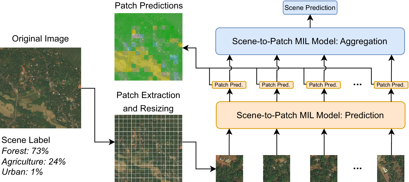
In our prior work, we proposed a novel approach for EO, where both scene- and patch-level predictions can be made while only requiring scene-level labels for training. This is achieved by reframing pixel-level segmentation as scene-level regression, where the objective is to predict the coverage proportion of each segmentation class. The motivation for such an approach is that scene-level labels are easy to procure (as they are summaries of the content of an image as opposed to detailed pixel-level annotations), which helps expedite the labeling process. Furthermore, it also reduces the likelihood of label errors, which often occur in EO segmentation datasets (Rakhlin et al., Reference Rakhlin, Davydow and Nikolenko2018). However, scene-level predictions cannot be used for segmentation. Therefore, it is necessary to have a model that learns from scene-level labels but can produce patch- or pixel-level predictions—our prior S2P approach achieved this by using inherently interpretable MIL models. We provide a high-level overview of our S2P approach in Figure 1 and discuss our model architecture in more detail in the next section.
MIL scene-to-patch overview. The model produces both instance (patch) and bag (scene) predictions but only learns from scene-level labels. Example from the DeepGlobe dataset (Section 4.1).
3.2. Single resolution scene-to-patch approach
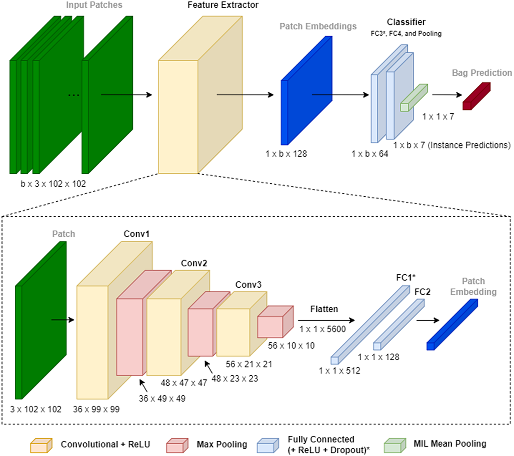
Our original S2P approach utilized an Instance Space Neural Network (known as mi-Net in Wang et al., Reference Wang, Yan, Tang, Bai and Liu2018), which operates at a single input and output resolution. In Figure 2, we give an example S2P architecture for the DeepGlobe dataset (Section 4.1), which has seven classes. The model takes a bag containing $ b $
instance patches as input, where each patch has three channels (red, green, and blue) and is 102 × 102 px. The patches are independently passed through a feature extractor, resulting in
$ b $
instance patches as input, where each patch has three channels (red, green, and blue) and is 102 × 102 px. The patches are independently passed through a feature extractor, resulting in $ b $
patch embeddings; each of length 128. These patch embeddings are then classified, and the mean of the patch predictions is used as the overall bag prediction. Note these models are trained end-to-end and only learn from scene-level (bag) labels—no patch-level labels are used during training.
$ b $
patch embeddings; each of length 128. These patch embeddings are then classified, and the mean of the patch predictions is used as the overall bag prediction. Note these models are trained end-to-end and only learn from scene-level (bag) labels—no patch-level labels are used during training.
S2P single-resolution model architecture. Note that some fully connected (FC) layers use ReLU and Dropout (denoted with *) while some do not, and $ b $
denotes bag size (number of patches).
$ b $
denotes bag size (number of patches).
Formally, for a collection of $ n $
EO images
$ n $
EO images $ \mathcal{X}=\left\{{X}_1,\dots, {X}_n\right\} $
, each image
$ \mathcal{X}=\left\{{X}_1,\dots, {X}_n\right\} $
, each image $ {X}_i\in \mathcal{X} $
has a corresponding scene-level label
$ {X}_i\in \mathcal{X} $
has a corresponding scene-level label $ {Y}_i\in \mathcal{Y} $
, where
$ {Y}_i\in \mathcal{Y} $
, where $ {Y}_i=\left\{{Y}_i^1,\dots, {Y}_i^C\right\} $
.
$ {Y}_i=\left\{{Y}_i^1,\dots, {Y}_i^C\right\} $
. $ C $
is the number of classes (e.g., types of land cover), and
$ C $
is the number of classes (e.g., types of land cover), and $ {Y}_i^c $
is the coverage proportion for class
$ {Y}_i^c $
is the coverage proportion for class $ c $
in image
$ c $
in image $ {X}_i $
, such that
$ {X}_i $
, such that $ {\sum}_{c=1}^C{Y}_i^c=1 $
. For each EO image
$ {\sum}_{c=1}^C{Y}_i^c=1 $
. For each EO image $ {X}_i\in \mathcal{X} $
, a set of
$ {X}_i\in \mathcal{X} $
, a set of $ b $
patches
$ b $
patches $ \left\{{x}_i^1,\dots, {x}_i^b\right\} $
is extracted, and our S2P models make a prediction
$ \left\{{x}_i^1,\dots, {x}_i^b\right\} $
is extracted, and our S2P models make a prediction $ {\hat{y}}_i^j $
for each patch. The mean of these patch-level predictions is then taken to make an overall scene-level prediction
$ {\hat{y}}_i^j $
for each patch. The mean of these patch-level predictions is then taken to make an overall scene-level prediction $ {\hat{Y}}_i=\frac{1}{b}{\sum}_{j=1}^b{\hat{y}}_i^j $
.
$ {\hat{Y}}_i=\frac{1}{b}{\sum}_{j=1}^b{\hat{y}}_i^j $
.
The configuration of our S2P model shown in Figure 2 uses three convolutional layers in the feature extractor model, but we also experiment with only using two convolution layers (see Supplementary Appendix C.3 for further details). The S2P models are relatively small (in comparison to baseline architectures such as ResNet18 and U-Net; see Supplementary Appendix C.1), which means they are less expensive to train and run. This reduces the GHG emission effect of model development and deployment, which is an increasingly important consideration for the use of ML (Kaack et al., Reference Kaack, Donti, Strubell, Kamiya, Creutzig and Rolnick2022). Furthermore, the S2P approach makes patch predictions inherently—post-hoc interpretability methods such as MIL local interpretations (Early et al., Reference Early, Evers and Ramchurn2022c) are not required.
Reframing EO segmentation as a regression problem does not necessitate a MIL approach; it can be treated as a traditional supervised regression problem. However, as EO images are often very high resolution, the images would have to be downsampled, and, as such, important data would be lost. With MIL, it is possible to operate at higher resolutions than a purely supervised learning approach. In our prior work, we experimented with different resolutions, but the S2P models were only able to operate at a single resolution. In the next section, we discuss our extension to S2P models which allows processing of multiple resolutions within a single model.
3.3. Multi-resolution scene-to-patch approaches
The objective of our S2P extension is to utilize multiple resolutions within a single model. While our prior work investigated the use of different resolutions, it only did so with separate models for each resolution. This does not allow information to be shared between different resolutions, which may hinder performance. For example, in aerial imagery, larger features such as a house might be easy to classify at lower resolutions (when the entire house fits in a single patch), but higher resolutions might be required to separate similar classes, such as the difference between trees and grass. Furthermore, a multi-resolution approach incorporates some notion of spatial relationships, helping to reduce the noise in high-resolution predictions (e.g., when a patch prediction is different from its neighbors). Combining multiple resolutions into a single model facilitates stronger performance and multi-resolution prediction (which aids interpretability) without the need to train separate models for different resolutions.
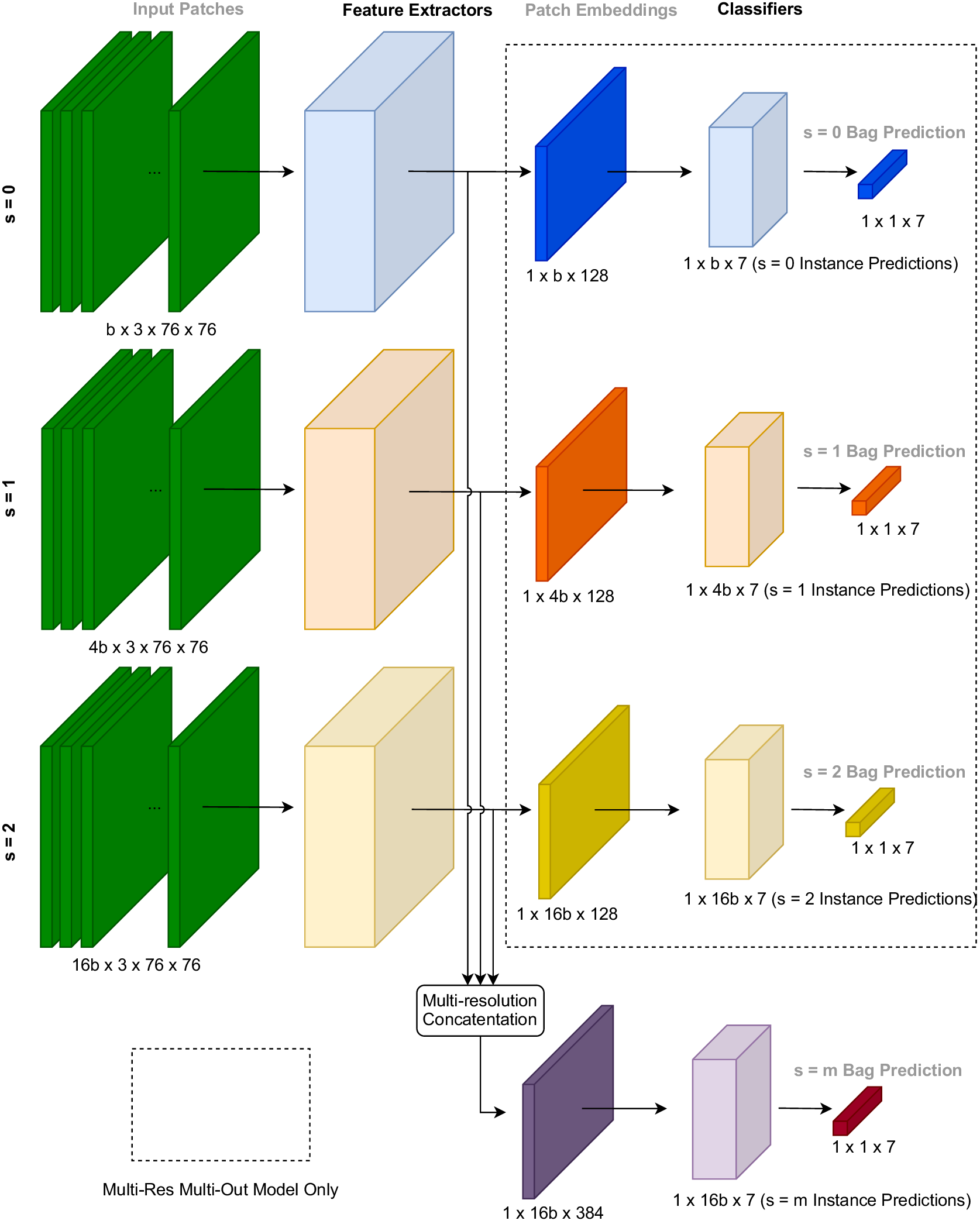
Several existing works have investigated multi-resolution MIL models, which we use as inspiration for our multi-resolution S2P models. Most notably, we base our approach on Multi-scale Domain-adversarial MIL (MS-DA-MIL; Hashimoto et al., Reference Hashimoto, Fukushima, Koga, Takagi, Ko, Kohno, Nakaguro, Nakamura, Hontani and Takeuchi2020) and Dual Stream MIL (DSMIL; Li et al., Reference Li, Li and Eliceiri2021). MS-DA-MIL uses a two-stage approach, where the latter stage operates at multiple resolutions and makes a combined overall prediction. DSMIL also uses a two-stage approach and provides a unique approach to combining feature embeddings extracted at different resolutions. Our novel method differs from these approaches in that it only uses a single stage of training. We extract patches at different resolutions and transform these patches into embeddings at each resolution using separate feature extractors (i.e., distinct convolutional layers for each resolution). This allows better extraction of features specific to each resolution (in comparison to using a single feature extractor for all resolutions, as done by Marini et al., Reference Marini, Otálora, Ciompi, Silvello, Marchesin, Vatrano, Buttafuoco, Atzori and Müller2021). We propose two different approaches for classification:
-
1. Multi-resolution single-out (MRSO)—This model uses multiple resolutions as input, but only makes predictions at the highest resolution. However, this high-resolution output uses information from all the input resolutions in its decision-making process.
-
2. Multi-resolution multi-out (MRMO)—This model uses multiple-resolution inputs and makes predictions at multiple resolutions. Given $ {s}_n $
input resolutions, it makes
$ {s}_n+1 $
sets of predictions: one independent set for each input resolution, and one main set, utilizing information from all input resolutions (as in the MRSO model).
$ {s}_n $
input resolutions, it makes
$ {s}_n+1 $
sets of predictions: one independent set for each input resolution, and one main set, utilizing information from all input resolutions (as in the MRSO model).


We give an example of the MRSO/MRMO models in Figure 3. Here, we utilize $ {s}_n=3 $
input resolutions:
$ {s}_n=3 $
input resolutions: $ s=0 $
,
$ s=0 $
, $ s=1 $
, and
$ s=1 $
, and $ s=2 $
, where each resolution is twice that of the previous. For MRMO, the individual resolution predictions are made independently (i.e., not sharing information between the different resolutions), but the main prediction,
$ s=2 $
, where each resolution is twice that of the previous. For MRMO, the individual resolution predictions are made independently (i.e., not sharing information between the different resolutions), but the main prediction, $ s=m $
, utilizes information from all input resolutions to make predictions at the
$ s=m $
, utilizes information from all input resolutions to make predictions at the $ s=2 $
scale. During MRMO training, we optimize the model to minimize the root mean square error (RMSE) averaged over all four outputs, aiming to achieve strong performance at each independent resolution as well as the combined resolution. MRSO does not make independent predictions at each scale, only the main
$ s=2 $
scale. During MRMO training, we optimize the model to minimize the root mean square error (RMSE) averaged over all four outputs, aiming to achieve strong performance at each independent resolution as well as the combined resolution. MRSO does not make independent predictions at each scale, only the main $ s=m $
predictions, meaning it can be trained using standard RMSE. In the next section, we discuss how we combine information across different resolutions for MRSO and MRMO.
$ s=m $
predictions, meaning it can be trained using standard RMSE. In the next section, we discuss how we combine information across different resolutions for MRSO and MRMO.
S2P multi-resolution architecture. The embedding process uses independent feature extraction modules (CNN layers, see Figure 2), allowing specialized feature extraction for each resolution. The MRMO configuration produces predictions at $ s=0 $
,
$ s=0 $
, $ s=1 $
,
$ s=1 $
, $ s=2 $
, and
$ s=2 $
, and $ s=m $
resolutions (indicated by the dashed box); MRSO only produces
$ s=m $
resolutions (indicated by the dashed box); MRSO only produces $ s=m $
predictions.
$ s=m $
predictions.
3.4. Multi-resolution MIL concatenation
In our multi-resolution models MRSO and MRMO, we combine information between different input resolutions to make more accurate predictions. To do so, we use an approach similar to Li et al. (Reference Li, Li and Eliceiri2021). A fundamental part of our approach is how patches are extracted at different resolutions: we alter the grid size, doubling it at each increasing resolution. This means a single patch of size $ p $
x
$ p $
x $ p $
px at resolution
$ p $
px at resolution $ s=0 $
is represented with four patches at resolution
$ s=0 $
is represented with four patches at resolution $ s=1 $
, each also of size
$ s=1 $
, each also of size $ p $
x
$ p $
x $ p $
px. As such, the same area is represented at twice the original resolution, that is,
$ p $
px. As such, the same area is represented at twice the original resolution, that is, $ 2p $
x
$ 2p $
x $ 2p $
px at
$ 2p $
px at $ s=1 $
compared to
$ s=1 $
compared to $ p $
x
$ p $
x $ p $
px at
$ p $
px at $ s=0 $
. Extending this to
$ s=0 $
. Extending this to $ s=2 $
follows the same process, resulting in 16 patches for each patch at
$ s=2 $
follows the same process, resulting in 16 patches for each patch at $ s=0 $
, that is, at four times the original resolution (
$ s=0 $
, that is, at four times the original resolution ( $ 4p $
x
$ 4p $
x $ 4p $
px). This process is visually represented on the left of Figure 4. As such, given a bag of size
$ 4p $
px). This process is visually represented on the left of Figure 4. As such, given a bag of size $ b $
at
$ b $
at $ s=0 $
, the equivalent bags at
$ s=0 $
, the equivalent bags at $ s=1 $
and
$ s=1 $
and $ s=2 $
are of size
$ s=2 $
are of size $ 4b $
and
$ 4b $
and $ 16b $
respectively, as shown in Figure 3.
$ 16b $
respectively, as shown in Figure 3.
Multi-resolution patch extraction and concatenation. Left: Patches are extracted at different resolutions, where each patch at scale $ s=0 $
has four corresponding
$ s=0 $
has four corresponding $ s=1 $
patches and 16 corresponding
$ s=1 $
patches and 16 corresponding $ s=2 $
patches. Right: The
$ s=2 $
patches. Right: The $ s=0 $
and
$ s=0 $
and $ s=1 $
embeddings are repeated to match the number of
$ s=1 $
embeddings are repeated to match the number of $ s=2 $
embeddings, and then concatenated to create multi-resolution embeddings.
$ s=2 $
embeddings, and then concatenated to create multi-resolution embeddings.
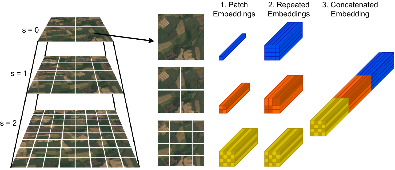
Given this multi-resolution patch extraction process, we then need to combine information across the different resolutions. We do so by using independent feature extraction modules (one per resolution, see Figure 3), which give a set of patch embeddings, one per patch, for each resolution. Therefore, we will have $ b $
embeddings at scale
$ b $
embeddings at scale $ s=0 $
,
$ s=0 $
, $ 4b $
embeddings at
$ 4b $
embeddings at $ s=1 $
, and
$ s=1 $
, and $ 16b $
embeddings at
$ 16b $
embeddings at $ s=2 $
. To combine these embeddings, we repeat the
$ s=2 $
. To combine these embeddings, we repeat the $ s=0 $
and
$ s=0 $
and $ s=1 $
embeddings to match the number of embeddings at
$ s=1 $
embeddings to match the number of embeddings at $ s=2 $
(16 repeats per embedding for
$ s=2 $
(16 repeats per embedding for $ s=0 $
and 4 repeats per embedding for
$ s=0 $
and 4 repeats per embedding for $ s=1 $
). This repetition preserves spatial relationships, such that the embeddings for lower resolutions (
$ s=1 $
). This repetition preserves spatial relationships, such that the embeddings for lower resolutions ( $ s=0 $
and
$ s=0 $
and $ s=1 $
) cover the same image regions as captured by the higher resolution
$ s=1 $
) cover the same image regions as captured by the higher resolution $ s=2 $
embeddings. Given the repeated embeddings, it is now possible to concatenate the embeddings from different resolutions, resulting in an extended embedding for each
$ s=2 $
embeddings. Given the repeated embeddings, it is now possible to concatenate the embeddings from different resolutions, resulting in an extended embedding for each $ s=2 $
embedding that includes information from
$ s=2 $
embedding that includes information from $ s=0 $
and
$ s=0 $
and $ s=1 $
. Note the embeddings extracted at each resolution are the same size (
$ s=1 $
. Note the embeddings extracted at each resolution are the same size ( $ l=128 $
), so the concatenated embeddings are three times as long (
$ l=128 $
), so the concatenated embeddings are three times as long ( $ 3l=384 $
). This process is summarized in Figure 4.
$ 3l=384 $
). This process is summarized in Figure 4.
4. Experiments
In this section, we detail our experiments, first describing the datasets (Section 4.1) and models (Section 4.2). We then provide our results (Section 4.3).
4.1. Datasets
We conduct experiments on two datasets: DeepGlobe (Demir et al., Reference Demir, Koperski, Lindenbaum, Pang, Huang, Basu, Hughes, Tuia and Raskar2018) and FloodNet (Rahnemoonfar et al., Reference Rahnemoonfar, Chowdhury, Sarkar, Varshney, Yari and Murphy2021). Both datasets are described in detail below.
DeepGlobe. Following our prior work (Early et al., Reference Early, Deweese, Evers and Ramchurn2022b), we use the DeepGlobe-LCC dataset (Demir et al., Reference Demir, Koperski, Lindenbaum, Pang, Huang, Basu, Hughes, Tuia and Raskar2018). It consists of 803 satellite images with three channels: red, green, and blue (RGB). Each image is 2448 × 2448 pixels with a 50 cm pixel resolution. All images were sourced from the WorldView3 satellite covering regions in Thailand, Indonesia, and India. Each image has a corresponding annotation mask, separating the images into 7 different land cover classes such as urban, agricultural, and forest. There are also validation and test splits with 171 and 172 images respectively, but as these splits did not include annotation masks, they were not used in this work.
FloodNet. To assess our S2P approach on EO data captured with aerial imagery, we use the FloodNet dataset (Rahnemoonfar et al., Reference Rahnemoonfar, Chowdhury, Sarkar, Varshney, Yari and Murphy2021). This dataset consists of 2343 high-resolution (4000 × 3000 px) RGB images of Ford Bend County in Texas, captured between August 30 and September 4, 2017 after Hurricane Harvey. Images were taken with DJI Mavic Pro quadcopters at 200 feet above ground level (flown by emergency responders as part of the disaster response process). The dataset aims to capture post-disaster flooding. Each image is segmented into 10 different classes, including flood-specific annotations such as flooded/non-flooded buildings, and flooded/non-flooded roads.
While both the DeepGlobe and FloodNet datasets provide pixel-level annotations, these segmentation labels are only used to generate the regression targets for training and for evaluating the predicted patch segmentation, that is, they are not directly used during training. However, we would like to stress that these segmentation labels are not strictly required for our approach, that is, the scene-level regression targets can be created without having to perform segmentation.
For the DeepGlobe dataset, due to its limited size (only 803 images), we used 5-fold cross-validation rather than the standard 10-fold approach. With this configuration, each fold had an 80/10/10 split for train/validation/test. The FloodNet dataset comes with pre-defined dataset splits: 1445 ( $ \sim 61.7\% $
) train, 450 (
$ \sim 61.7\% $
) train, 450 ( $ \sim 19.2\% $
) validation, and 448 (
$ \sim 19.2\% $
) validation, and 448 ( $ \sim 19.1\% $
) test, which were used consistently in five training repeats (i.e., no cross-validation). For more details on both datasets, see Supplementary Appendix B.
$ \sim 19.1\% $
) test, which were used consistently in five training repeats (i.e., no cross-validation). For more details on both datasets, see Supplementary Appendix B.
4.2. Model configurations
To apply MIL at different resolutions, we alter the grid size applied over the image (i.e., the number of extracted patches). For the DeepGlobe dataset (square images), we used three grid sizes: 8 × 8, 16 × 16, and 32 × 32. For the FloodNet dataset (non-square images), we used 8 × 6, 16 × 12, and 32 × 24. These grid sizes are chosen such that they can be used directly for three different resolutions in the multi-resolution models, for example, 32 × 32 ( $ s=2 $
) is twice the resolution of 16 × 16 (
$ s=2 $
) is twice the resolution of 16 × 16 ( $ s=1 $
), which is twice the resolution of 8 × 8 (
$ s=1 $
), which is twice the resolution of 8 × 8 ( $ s=0 $
).
$ s=0 $
).
We also compare our MIL S2P models to a fine-tuned ResNet18 model (He et al., Reference He, Zhang, Ren and Sun2016), and two U-Net variations operating on different image sizes (224 × 224 px and 448 × 448 px). These baseline models are trained in the same manner as the S2P models, that is, using scene-level regression. Although the ResNet model does not produce patch- or pixel-level predictions, we use it as a scene-level baseline as many existing LCC approaches utilize ResNet architectures (Hoeser et al., Reference Hoeser, Bachofer and Kuenzer2020; Hoeser and Kuenzer, Reference Hoeser and Kuenzer2020; Rahnemoonfar et al., Reference Rahnemoonfar, Chowdhury, Sarkar, Varshney, Yari and Murphy2021). For the U-Net models, we follow the same procedure as Wang et al. (Reference Wang, Chen, Xie, Azzari and Lobell2020) and use class activation maps to recover segmentation outputs. This means U-Net is a stronger baseline than ResNet as it can be used for both scene- and pixel-level prediction. For more details on the implementation, models, and training process, see Supplementary Appendices A and C.
4.3. Results
We evaluate performance on both datasets using four metrics, covering scene-, patch-, and pixel-level prediction. Scene-level performance is scored using root mean square error (RMSE) and mean absolute error (MAE), where lower values are better. Both of these metrics compare the scene-level (bag) predictions with the true scene-level coverage labels. For patch-level predictions, we report the patch-level mean Intersection over Union (mIoU; Everingham et al., Reference Everingham, Gool, Williams, Winn and Zisserman2010; Minaee et al., Reference Minaee, Boykov, Porikli, Plaza, Kehtarnavaz and Terzopoulos2021), where larger values are better.Footnote 1 Patch labels (only used during evaluation; not during training) are derived from the true segmentation masks, where the labels are the class that has maximum coverage in each patch. For pixel-level prediction, we compute pixel-level mIoU using the original ground-truth segmentation masks.Footnote 2 For S2P models, this is achieved by resizing the patch-level segmentation output to the same size as the ground-truth segmentation mask. Pixel-level mIoU is the primary metric for evaluation as it best determines the ability of the models to segment the input images—patch-level evaluation is dependent on the grid size so is not a consistent metric across different resolutions (but can be useful to compare patch-level predictions at the same resolution). Strong models should perform well at both scene- and pixel-level prediction, that is, low scene RMSE, low scene MAE, and high pixel mIoU.
Our results are given in Tables 1 and 2 for DeepGlobe and FloodNet respectively. We compare the three non-MIL baselinesFootnote
3 (ResNet18, U-Net 224, and U-Net 448) with S2P single resolution (SR) models operating at three different scales ( $ s=0 $
,
$ s=0 $
, $ s=1 $
, and
$ s=1 $
, and $ s=2 $
), the S2P MRSO approach, and the S2P MRMO approach (evaluating the MRMO outputs at all scales). Our first observation is that, for both datasets, all of our S2P models outperform the baseline approaches at both scene- and pixel-level prediction, showing the efficacy of our S2P approach. We also find that, out of all the methods, the MRMO approach achieves the best performance when using its combined
$ s=2 $
), the S2P MRSO approach, and the S2P MRMO approach (evaluating the MRMO outputs at all scales). Our first observation is that, for both datasets, all of our S2P models outperform the baseline approaches at both scene- and pixel-level prediction, showing the efficacy of our S2P approach. We also find that, out of all the methods, the MRMO approach achieves the best performance when using its combined $ s=m $
output, demonstrating the performance gain of using multiple resolutions. Note the MRMO
$ s=m $
output, demonstrating the performance gain of using multiple resolutions. Note the MRMO $ s=m $
performance is better than the MRSO
$ s=m $
performance is better than the MRSO $ s=m $
performance, suggesting that optimizing the model for independent scale predictions (
$ s=m $
performance, suggesting that optimizing the model for independent scale predictions ( $ s=0 $
,
$ s=0 $
, $ s=1 $
, and
$ s=1 $
, and $ s=2 $
) as well as the combined output (
$ s=2 $
) as well as the combined output ( $ s=m $
) is beneficial for learning—the multi-output nature potentially leads to better representation learning at each individual scale and could be helpful in avoiding overfitting. However, the MRSO model still outperforms its single-resolution equivalent (S2P SR
$ s=m $
) is beneficial for learning—the multi-output nature potentially leads to better representation learning at each individual scale and could be helpful in avoiding overfitting. However, the MRSO model still outperforms its single-resolution equivalent (S2P SR $ s=2 $
), again demonstrating the efficacy of using multiple resolutions.
$ s=2 $
), again demonstrating the efficacy of using multiple resolutions.
DeepGlobe results
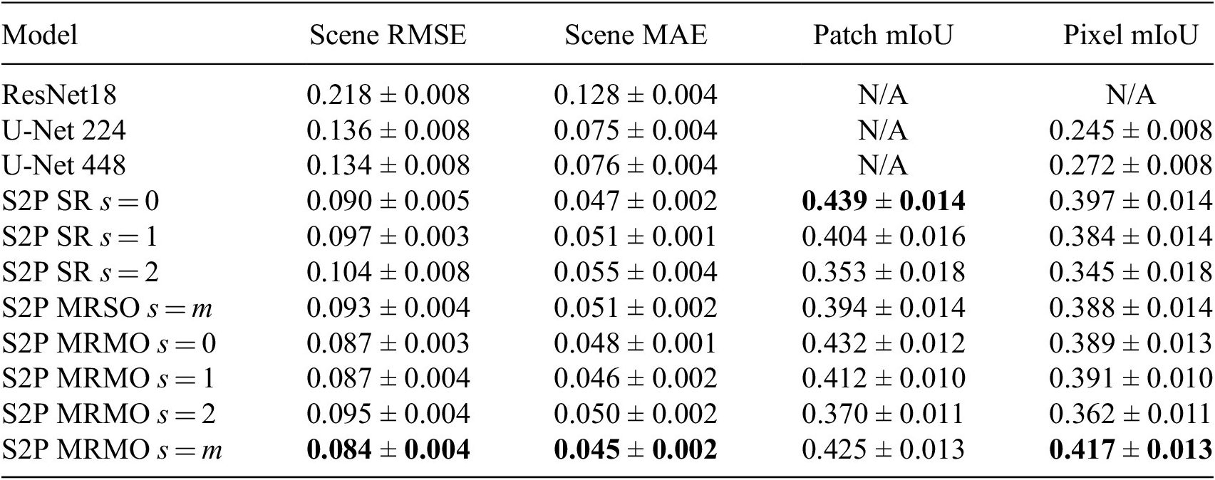
Note: We give the mean performance averaged over five repeat training runs, with bounds using standard error of the mean. Best performance for each metric is indicated in bold.
FloodNet results
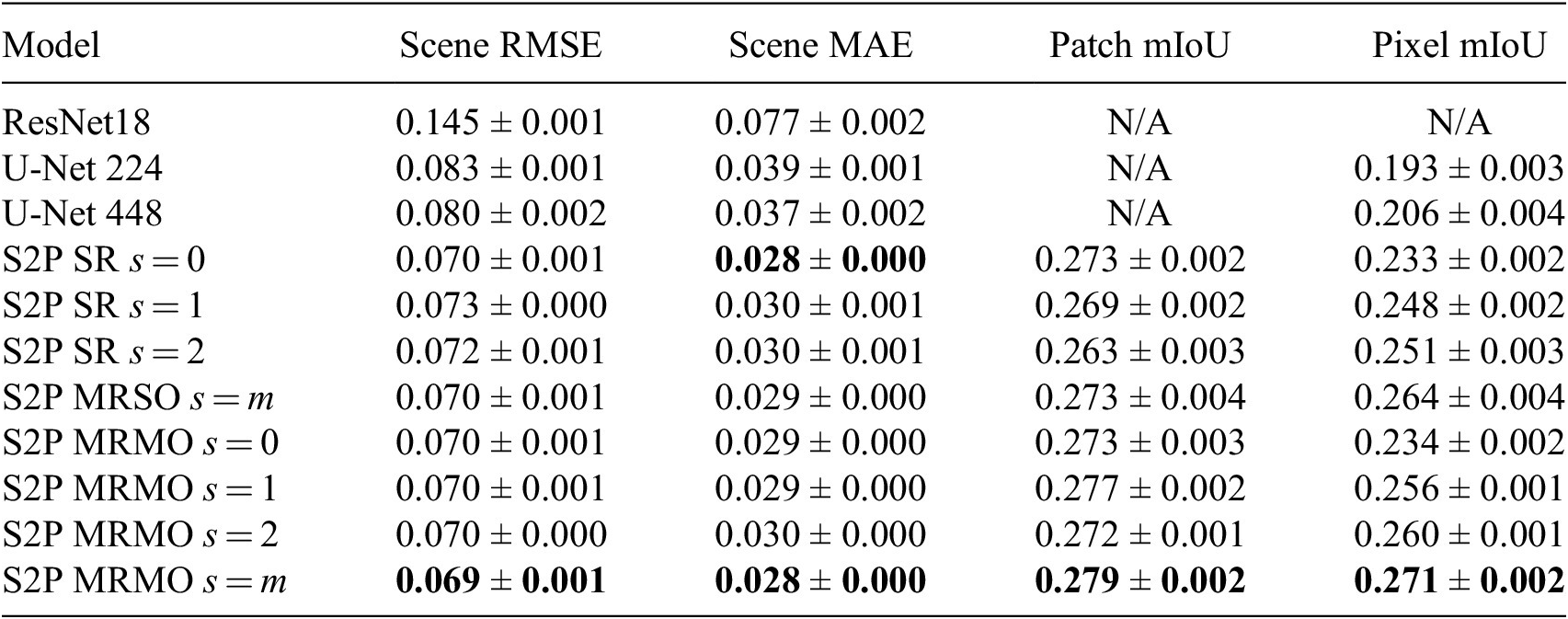
Note: We give the mean performance averaged over five repeat training runs, with bounds using standard error of the mean. Best performance for each metric is indicated in bold.
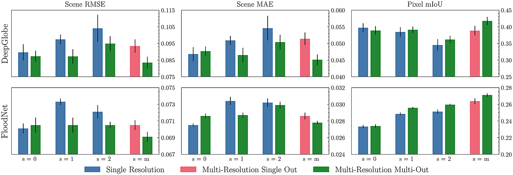
To compare the change in performance caused by using different/multiple resolutions, we visualize our S2P results in Figure 5. For the DeepGlobe dataset, when using single-resolution models, we observe that increasing the resolution leads to worse performance (greater Scene RMSE and MAE, and lower Pixel mIoU). In our prior work, we identified this as a trade-off between performance and segmentation resolution. However, with the extension to multi-resolution models, it is possible to achieve strong performance while operating at higher resolutions, overcoming this trade-off. For the FloodNet dataset, we observe the opposite trend for pixel mIoU—increasing resolution leads to better segmentation performance, even for the single resolution models. This is likely explained by the different spatial modalities of the two datasets: DeepGlobe images cover much larger spatial areas (e.g., entire towns and fields in a single image) compared to FloodNet (e.g., a handful of buildings or a single road per image). As such, the FloodNet segmentation masks identify individual objects (e.g., a single tree), which require high-resolution inputs and outputs to correctly separate (as opposed to broadly segmenting a forest region as in DeepGlobe). However, we still observe that utilizing multiple resolutions gives better performance for FloodNet. We also find that the MRMO independent resolution predictions ( $ s=0 $
,
$ s=0 $
, $ s=1 $
, and
$ s=1 $
, and $ s=2 $
) typically outperform the equivalent single-resolution model predictions.
$ s=2 $
) typically outperform the equivalent single-resolution model predictions.
S2P resolution comparison. We compare model performance for scene RMSE (left), scene MAE (middle), and pixel mIoU (right) for both DeepGlobe (top) and FloodNet (bottom).
5. Discussion
In this section, we further discuss our findings. First, we analyze the model predictions in more detail (Section 5.1), then investigate the interpretability and segmentation outputs of the models (Section 5.2). Next, we conduct an ablation study into model architectures (Section 5.3). Finally, we discuss the limitations of this study and outline areas for future work (Section 5.4).
5.1. Model analysis
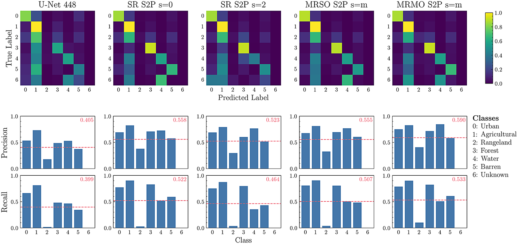
We conduct an additional study to further analyze and compare the effectiveness of the different approaches. We use confusion matrices along with precision and recall analysis to investigate the performance of the models on particular classes. The results for the DeepGlobe dataset are presented in Figure 6. We observe that all of the analyzed models perform best on the agricultural, urban, and forest classes, but struggle on rangeland and unknown classes. For the MRMO $ s=m $
model (the best-performing approach) rangeland is most often predicted as agricultural, and unknown is most often predicted as water or agricultural. Rangeland is defined as any green land or grass that is not forest or farmland, so is often difficult to separate from agricultural land. The unknown class is very underrepresented in the dataset compared to the other classes (see Supplementary Appendix B.1). We note that the MRMO
$ s=m $
model (the best-performing approach) rangeland is most often predicted as agricultural, and unknown is most often predicted as water or agricultural. Rangeland is defined as any green land or grass that is not forest or farmland, so is often difficult to separate from agricultural land. The unknown class is very underrepresented in the dataset compared to the other classes (see Supplementary Appendix B.1). We note that the MRMO $ s=m $
model also achieves the best macro-averaged precision and recall.
$ s=m $
model also achieves the best macro-averaged precision and recall.
DeepGlobe model analysis. Top: Row normalized confusion matrices. Bottom: Classwise precision and recall, where the dotted line indicates the macro-averaged performance (which is also denoted in the top right corner of each plot).
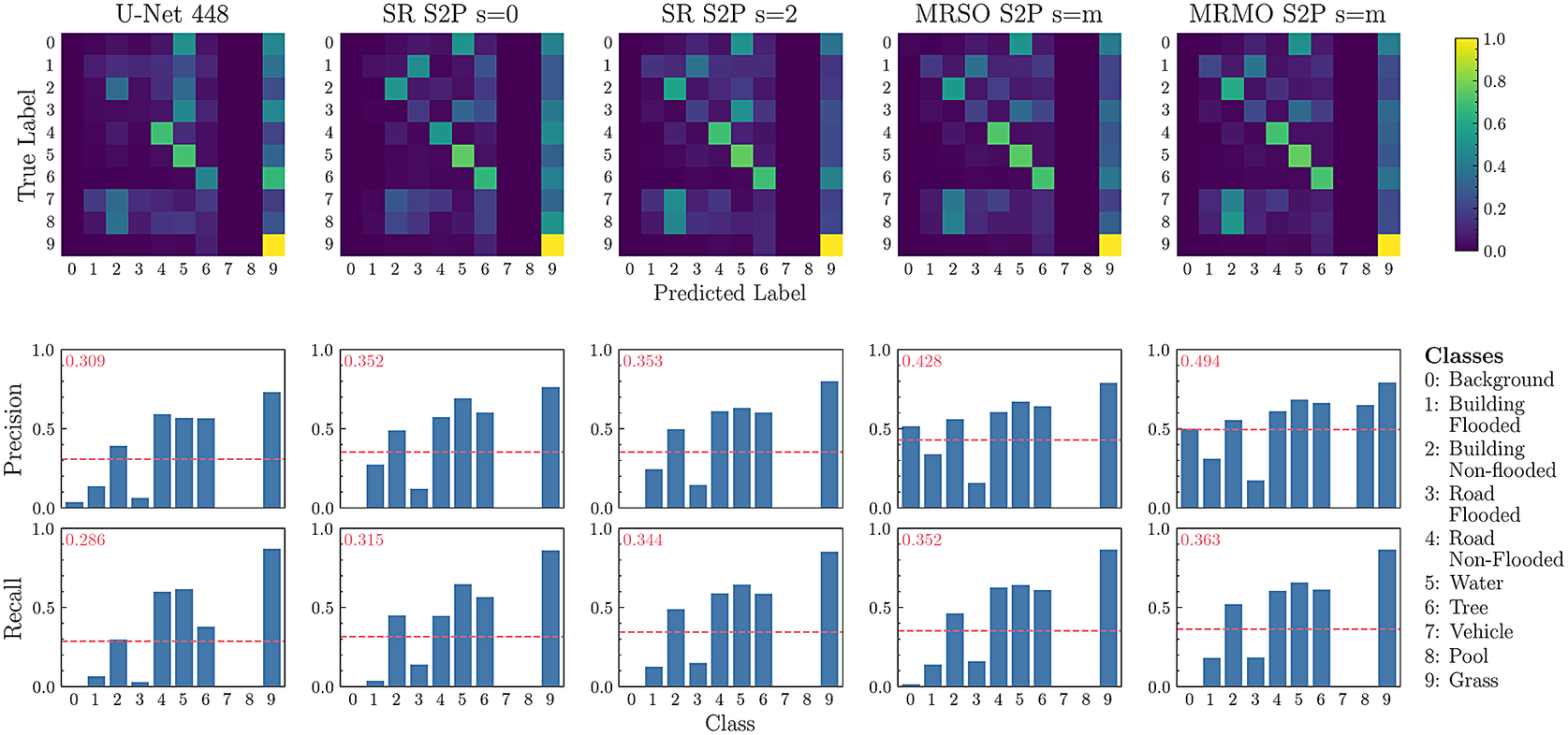
In a similar study for FloodNet (Figure 7), the models perform best at identifying the road non-flooded, water, tree, and grass classes, but struggle on the background, vehicle, and pool classes. The vehicle and pool classes represent relatively small objects (compared to buildings and roads) and are also very underrepresented (see Supplementary Appendix B.2), making them hard to identify. However, they are most often classified as building non-flooded, which is an appropriate alternative prediction (i.e., better than classifying them as natural objects such as trees). The background category is a catch-all for any regions that do not belong to the other classes, but it often contains elements of the other classes, making it difficult to segment. Again, we find that the MRMO $ s=m $
model has the best precision and recall performance.
$ s=m $
model has the best precision and recall performance.
FloodNet model analysis. Top: Row normalized confusion matrices. Bottom: Classwise precision and recall, where the dotted line indicates the macro-averaged performance (which is also denoted in the top left corner of each plot).
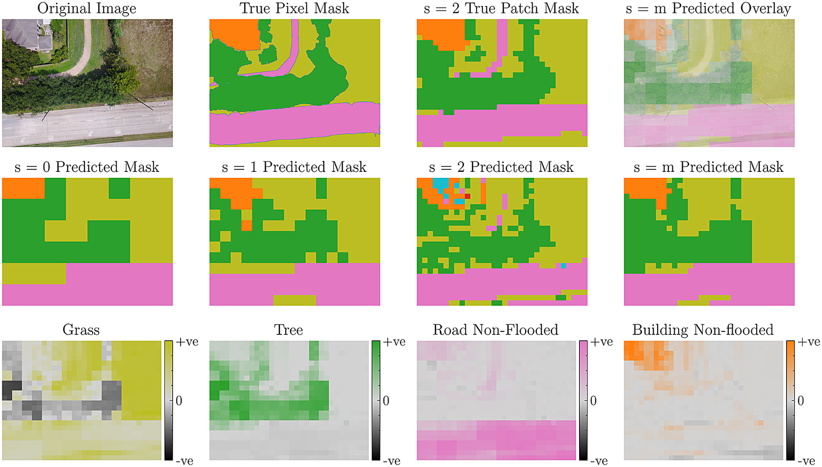
5.2. Model interpretability
As our S2P models inherently produce patch-level predictions, we can directly interpret their segmentation outputs. In Figure 8, we do so for the MRMO model on the FloodNet dataset. We observe that the model is able to accurately separate the non-flooded building and road, and also identifies the grass and trees. Furthermore, we find the $ s=m $
predictions are an improvement over the independent predictions, notably that the
$ s=m $
predictions are an improvement over the independent predictions, notably that the $ s=m $
output is less noisy than the
$ s=m $
output is less noisy than the $ s=2 $
predictions. We also note that the model is also to support and refute different classes, which further aids interpretability.
$ s=2 $
predictions. We also note that the model is also to support and refute different classes, which further aids interpretability.
MRMO interpretability example. Top (from left to right): the original dataset image; the true pixel-level mask; the true patch-level mask at resolution $ s=2 $
; the predicted mask from the MRMO model overlaid on the original image. Middle: Predicted masks for each of the MRMO outputs. Bottom: MRMO
$ s=2 $
; the predicted mask from the MRMO model overlaid on the original image. Middle: Predicted masks for each of the MRMO outputs. Bottom: MRMO $ s=m $
predicted masks for each class, showing supporting (+ve) and refuting regions (−ve).
$ s=m $
predicted masks for each class, showing supporting (+ve) and refuting regions (−ve).
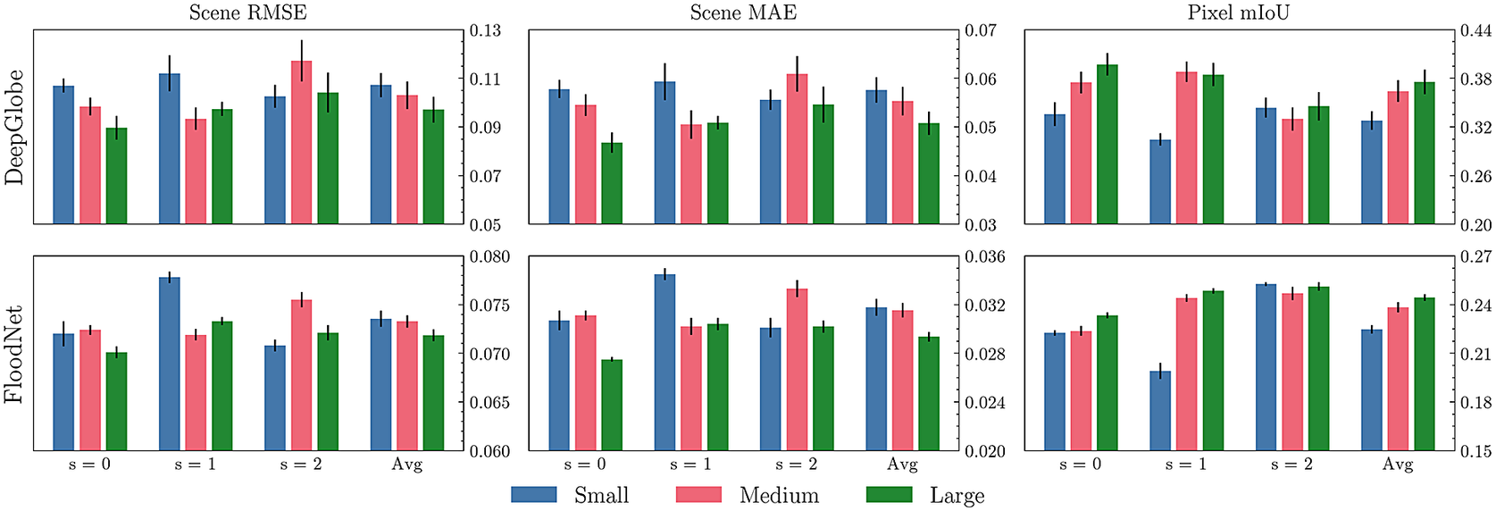
5.3. Ablation study: Single resolution S2P configurations
In our prior work (Early et al., Reference Early, Deweese, Evers and Ramchurn2022b), we experimented with changing the patch size: the dimensions to which each cell from the grid extraction process is resized. This influences the effective resolution (i.e., the level of downsampling) at which the S2P models are operating, and also impacts the MIL model architectures. We continue this analysis here, applying it to both DeepGlobe and FloodNet. We conducted an ablation study using three different patch sizes (small, medium, and large). This was done for each of three resolutions $ s=0 $
,
$ s=0 $
, $ s=1 $
, and
$ s=1 $
, and $ s=2 $
, resulting in nine different S2P single-resolution configurations (for further details, see Supplementary Appendix C.1). As shown in Figure 9, we find that the large model configuration has the best average performance on all metrics for both datasets. This matches our intuition that operating at higher resolutions leads to better performance. Given these results, we used the large configuration as the backbone of the multi-resolution S2P models, and as the choice of single-resolution model in our main results (Tables 1 and 2).
$ s=2 $
, resulting in nine different S2P single-resolution configurations (for further details, see Supplementary Appendix C.1). As shown in Figure 9, we find that the large model configuration has the best average performance on all metrics for both datasets. This matches our intuition that operating at higher resolutions leads to better performance. Given these results, we used the large configuration as the backbone of the multi-resolution S2P models, and as the choice of single-resolution model in our main results (Tables 1 and 2).
Single-resolution S2P ablation study. We observe that, on average, the large configuration achieves the best performance (lowest RMSE, lowest MAE, and highest mIoU) on both datasets. Error bars are given representing the standard error of the mean from five repeats.
5.4. Limitations and future work
While our new multi-resolution S2P approach outperforms existing methods, there are still limitations to the method. For the DeepGlobe dataset, the model struggles to separate rangeland and agricultural regions, and for the FloodNet dataset, it struggles to correctly separate flooded regions and identify smaller objects such as pools and vehicles. These problems mostly stem from dataset imbalance; future work could investigate dataset balancing or augmentation to overcome these class imbalances. It could also be beneficial to extend the MIL models to incorporate additional spatial information—this could help separate small objects from the larger objects they often appear next to, for example, swimming pools from houses. Potential solutions include utilizing positional embeddings (Vaswani et al., Reference Vaswani, Shazeer, Parmar, Uszkoreit, Jones, Gomez, Kaiser and Polosukhin2017), MIL attention (Ilse et al., Reference Ilse, Tomczak and Welling2018), or graph neural networks (Tu et al., Reference Tu, Huang, He and Zhou2019).
When considering the application of our work to other datasets, there are two points to consider. First, while our solution will scale to datasets containing more images of a similar size to the ones studied in this work, there could be resource issues when using datasets containing larger images (i.e., images larger than 4000 × 3000 px). The computational resources required are determined by the image size, the model’s architecture, and the effective resolution at which the model is operating (see Supplementary Appendix C). Reducing the model complexity or lowering the image resolution would overcome potential issues. However, we did not run into any such issues in our work (see Supplementary Appendix A for details on our compute resources). Second, in this work, we used datasets with existing segmentation labels that are converted into scene-level coverage labels. An area for future work is to investigate how to generate coverage labels for datasets without segmentation labels. This could also incorporate an analysis of model performance in the presence of label noise, that is, imperfect coverage labels.
Finally, we only tuned training hyperparameters on the DeepGlobe dataset (see Supplementary Appendix C.2 for more details). This was an intentional choice, as it allowed us to demonstrate that the hyperparameters found through tuning were robust (i.e., useful default parameters for training on other datasets). However, potentially better performance could be achieved on FloodNet by tuning the training hyperparameters specifically for that dataset and optimizing the model architectures as well as the training hyperparameters.
6. Conclusion
In this work, we presented a novel method for segmenting EO RS images. Our method extends our previous single-resolution S2P approach to multiple resolutions, which leads to improved performance and interpretability. We demonstrated the efficacy of our approach on two datasets: DeepGlobe (LCC from satellite imagery) and FloodNet (NDR from aerial imagery). As our S2P approaches do not require segmentation labels, faster and easier curation of larger and more diverse datasets can be achieved, facilitating the wider use of ML for climate change mitigation in technology, government, and academia.
Acknowledgements
We would like to thank the University of Southampton and the Alan Turing Institute for their support. The authors acknowledge the use of the University of Southampton IRIDIS high-performance computing facilities and associated support services. Finally, this work was supported by the Climate Change AI (CCAI) Mentorship Program.
Author contribution
Conceptualization: J.E.; Methodology: J.E.; Implementation: J.E.; Data visualization: J.E.; Writing (original draft): J.E.; Writing (editing and review): J.E. and Y.-J. C.D.; Supervision: Y.-J. C.D., C.E., and S.R.
Competing interest
The authors declare no competing interests exist.
Data availability statement
Code and trained models are available at https://github.com/JAEarly/MIL-Multires-EO (for more details, see Supplementary Appendix A). All data are openly available: DeepGlobe at https://www.kaggle.com/datasets/balraj98/deepglobe-land-cover-classification-dataset and FloodNet at https://github.com/BinaLab/FloodNet-Supervised_v1.0 (for more details, see Supplementary Appendix B).
Ethics statement
The research meets all ethical guidelines, including adherence to the legal requirements of the study country.
Funding statement
This work was funded by the AXA Research Fund and the UKRI TAS Hub (EP/V00784X/1). Both funders had no role in the study design, data collection and analysis, decision to publish, or preparation of the manuscript.
Supplementary material
The supplementary material for this article can be found at http://doi.org/10.1017/eds.2023.30.


 Open access