


Impact Statement
This new likelihood-based metric enables assessing physically relevant fine-scale structures in high-resolution climate simulations, complementing existing evaluation methods and guiding the improvement of next-generation climate models. This can enable more accurate climate projections, better suited to guide policy, and societal responses to climate change.
1. Introduction
Global km-scale models are the frontier in climate modeling, simulating the atmosphere and ocean at an unprecedented resolution of 10 km or less, with previously inaccessible physical detail (Stevens et al., Reference Stevens, Satoh, Auger, Biercamp, Bretherton, Chen, Düben, Judt, Khairoutdinov, Klocke, Kodama, Kornblueh, Lin, Neumann, Putman, Röber, Shibuya, Vanniere, Vidale, Wedi and Zhou2019). They are being developed to address long-standing limitations of low-resolution models, which operate at grid spacings of around 100 km and rely on parameterizations to approximate unresolved processes such as convection, cloud formation, and ocean eddies—approximations that drive major systematic errors and biases. By resolving these processes more explicitly, km-scale models could substantially improve the accuracy of global and regional climate projections. However, significant uncertainties remain due to parameterizations of remaining subgrid-scale processes. To isolate, understand, and reduce these biases, km-scale models need to be thoroughly evaluated.
Satellite observations are essential for evaluating km-scale models. A model that cannot reproduce the characteristics of today’s climate cannot be trusted to realistically simulate future changes under increased atmospheric carbon dioxide. Kilometer-scale models simulate one possible trajectory of the weather over many decades. The spatial and temporal statistics of this simulated time series dataset define the model’s climate and should be consistent with observations. However, since weather is intrinsically stochastic, individual simulated snapshots are not expected to match observed snapshots at that exact time. Instead, the problem of climate model evaluation is to determine whether the model reproduces the statistical properties of the observed climate system.
Traditionally, climate models are assessed by comparing spatio-temporally averaged outputs to observations using skill metrics such as mean-square error, variance, or correlation (Gleckler et al., Reference Gleckler, Taylor and Doutriaux2008; Flato et al., Reference Flato, Marotzke, Abiodun, Braconnot, Chou, Collins, Cox, Driouech, Emori, Eyring, Forest, Gleckler, Guilyardi, Jakob, Kattsov, Reason, Rummukainen, Stocker, Qin, G.-K., Tignor, Allen, Boschung, Nauels, Xia, Bex and Midgley2013). Spectral analyses directly compare variance across spatial and temporal scales (e.g., Fraedrich and Blender, Reference Fraedrich and Blender2003; Fredriksen and Rypdal, Reference Fredriksen and Rypdal2016). While informative, such metrics cannot account for the inherent randomness of climate fields and disregard the high-resolution spatio-temporal structure that encodes essential information about underlying physical processes (Labe and Barnes, Reference Labe and Barnes2022). More comprehensive statistical approaches compare models and observations as random processes or spatial fields but are limited to one-dimensional time series, long-term averaged fields, or coarse spatial scales (e.g., Lund and Li, Reference Lund and Li2009; Zhang and Shao, Reference Zhang and Shao2015). Recent methods such as the spherical convolutional Wasserstein distance (SCWD) introduce spatially aware distributional comparisons, yet still cannot capture fine-scale spatial structures relevant for km-scale models (Garrett et al., Reference Garrett, Harris, Li and Wang2024).
Process-oriented diagnostics have been developed to explicitly target key physical structures, particularly for deep convection. Organization indices such as
$ {I}_{org} $
 (Tompkins and Semie, Reference Tompkins and Semie2017) quantify convective clustering and have been widely applied to both models and observations (e.g., Bony et al., Reference Bony, Semie, Kramer, Soden, Tompkins and Emanuel2020). Lagrangian tracking of mesoscale convective systems enables comparisons of storm frequency, size, and lifecycle statistics against satellite climatologies (Feng et al., Reference Feng, Leung, Liu, Wang, Houze, Li, Hardin, Chen and Guo2021) but is typically limited to case studies of specific regions and sensitive to tracking algorithm design choices (Prein et al., Reference Prein, Feng, Fiolleau, Moon, Núñez Ocasio, Kukulies, Roca, Varble, Rehbein, Liu, Ikeda, Mu and Rasmussen2024).
Recent machine-learning–based approaches have begun to automate the evaluation of (km-scale) climate models, demonstrating the potential of computer vision and representation learning methods (Labe and Barnes, Reference Labe and Barnes2022; Brunner and Sippel, Reference Brunner and Sippel2023; Mooers et al., Reference Mooers, Pritchard, Beucler, Srivastava, Mangipudi, Peng, Gentine and Mandt2023). However, existing studies rely on global snapshots, spatial or temporal averaging, or variables that are not directly observable, limiting their interpretability and applicability for model evaluation against observations. To improve models, performance must be explicitly linked to physical processes that are localized in space and time, requiring local diagnostics of the statistical consistency between models and observations.
Hence, a robust evaluation metric for high-resolution climate models is needed that (1) assesses models based on the statistics of simulated fields, without requiring paired simulations; (2) is local in time, avoiding temporal averaging; (3) is local in space, avoiding both spatial averaging or only assessing large areas at once; (4) evaluates a field directly observable (or closely related to those observable) by satellites; (5) primarily evaluates the structures present in the field, rather than trivial differences in means or other low-order statistics; and (6) provides a quantitative difference metric that enables direct comparison across different model outputs.
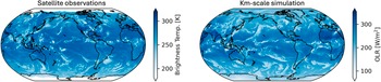
To address this gap, we introduce a statistically motivated metric for evaluating km-scale climate models directly against snapshots of satellite imagery. We first reproject observations and model outputs onto a grid suitable to train neural networks. Then, we train a generative model on observational data to learn a statistical representation of the climate system. We evaluate km-scale simulations based on the divergence of likelihood distributions of simulations and observations, estimated from the trained model. We present a case study evaluation of two state-of-the-art km-scale models, the Integrated Forecasting System coupled to the FESOM ocean–sea ice model (IFS-FESOM, Rackow et al., Reference Rackow, Pedruzo-Bagazgoitia, Becker, Milinski, Sandu, Aguridan, Bechtold, Beyer, Bidlot, Boussetta, Deconinck, Diamantakis, Dueben, Dutra, Forbes, Ghosh, Goessling, Hadade, Hegewald, Jung, Keeley, Kluft, Koldunov, Koldunov, Kölling, Kousal, Kühnlein, Maciel, Mogensen, Quintino, Polichtchouk, Reuter, Sármány, Scholz, Sidorenko, Streffing, Sützl, Takasuka, Tietsche, Valentini, Vannière, Wedi, Zampieri and Ziemen2025), and the ICOsahedral Nonhydrostatic model (ICON, Hohenegger et al., Reference Hohenegger, Korn, Linardakis, Redler, Schnur, Adamidis, Bao, Bastin, Behravesh, Bergemann, Biercamp, Bockelmann, Brokopf, Brüggemann, Casaroli, Chegini, Datseris, Esch, George, Giorgetta, Gutjahr, Haak, Hanke, Ilyina, Jahns, Jungclaus, Kern, Klocke, Kluft, Kölling, Kornblueh, Kosukhin, Kroll, Lee, Mauritsen, Mehlmann, Mieslinger, Naumann, Paccini, Peinado, Praturi, Putrasahan, Rast, Riddick, Roeber, Schmidt, Schulzweida, Schütte, Segura, Shevchenko, Singh, Specht, Stephan, von Storch, Vogel, Wengel, Winkler, Ziemen, Marotzke and Stevens2023), against observations from NOAA’s Geostationary Operational Environmental Satellite (GOES-16, Schmit and Gunshor, Reference Schmit, Gunshor, Goodman, Schmit, Daniels and Redmon2020). We focus on convective thunderstorm clouds, which are a major source of uncertainty in climate projections (Stephens et al., Reference Stephens, Shiro, Hakuba, Takahashi, Pilewskie, Andrews, Stubenrauch and Wu2024). We analyze outgoing longwave radiation (OLR), a quantity observable from satellites and commonly used as a proxy for high cloud cover and convective activity (Figure 1).
Example high-resolution snapshots of satellite observations and climate model simulations. Left: globally merged geostationary satellite image (11 μm brightness temperature) from the preliminary ISCCP-ng dataset (CIMSS, 2025). Right: outgoing longwave radiation (OLR) field simulated by the nextGEMS ICON model (Segura et al., Reference Segura, Pedruzo-Bagazgoitia, Weiss, Müller, Rackow, Lee, Dolores-Tesillos, Benedict, Aengenheyster, Aguridan, Arduini, Baker, Bao, Bastin, Baulenas, Becker, Beyer, Bockelmann, Brüggemann, Brunner, Cheedela, Das, Denissen, Dragaud, Dziekan, Ekblom, Engels, Esch, Forbes, Frauen, Freischem, García-Maroto, Geier, Gierz, González-Cervera, Grayson, Griffith, Gutjahr, Haak, Hadade, Haslehner, ul Hasson, Hegewald, Kluft, Koldunov, Koldunov, Kölling, Koseki, Kosukhin, Kousal, Kuma, Kumar, Li, Maury, Meindl, Milinski, Mogensen, Niraula, Nowak, Praturi, Proske, Putrasahan, Redler, Santuy, Sármány, Schnur, Scholz, Sidorenko, Spät, Sützl, Takasuka, Tompkins, Uribe, Valentini, Veerman, Voigt, Warnau, Wachsmann, Wacławczyk, Wedi, Wieners, Wille, Winkler, Wu, Ziemen, Zimmermann, Bender, Bojovic, Bony, Bordoni, Brehmer, Dengler, Dutra, Faye, Fischer, van Heerwaarden, Hohenegger, Järvinen, Jochum, Jung, Jungclaus, Keenlyside, Klocke, Konow, Klose, Malinowski, Martius, Mauritsen, Mellado, Mieslinger, Mohino, Pawłowska, Peters-von Gehlen, Sarré, Sobhani, Stier, Tuppi, Vidale, Sandu and Stevens2025).
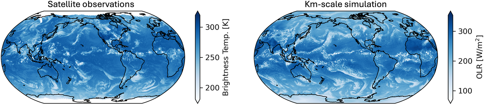
Figure 1. Long description
Two panels show global atmospheric data in a Robinson projection.
Left panel titled Satellite observations. The map displays brightness temperature in Kelvin. High brightness temperatures are shown in dark blue, while lower temperatures, representing cloud cover, are in white and light blue. Cloud patterns are concentrated along the equator and in swirling formations across the mid-latitudes. To the right of the map is a vertical color bar ranging from 200 to 300 Kelvin, labeled Brightness Temp. K.
Right panel titled Km-scale simulation. The map displays O L R in Watts per meter-squared. The visual pattern closely mimics the left panel, showing fine-scale convective structures and cloud filaments. Dark blue represents high O L R values, while white represents low O L R values associated with high-altitude clouds. To the right of the map is a vertical color bar ranging from 100 to 300, labeled O L R W forward slash m super 2.
2. Methods: likelihood-based evaluation of km-scale models
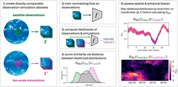
The key question that climate model evaluation aims to answer is how well model datasets represent the real climate system. To answer this question, we need to determine how similar the distribution of the model data is to observational data. Since the data is high-dimensional, calculating the similarity between two such datasets is not straightforward. For this purpose, we propose an evaluation framework based on the likelihood function of a generative image model (Figure 2). It is trained on an observational dataset to learn its statistical distribution and then places simulated data within this statistical distribution for comparison. Finally, the similarity between models and observations is calculated using symmetrized Kullback–Leibler (KL) divergence of their likelihood distributions. This produces a quantitative similarity metric suitable for evaluating km-scale models.
An overview of our likelihood-based framework for km-scale climate model evaluation. (1) We remap model and observation datasets onto the HEALPix projection to extract square patches for processing by the generative model. (2) A normalizing flow model is trained on observations only and (3) used to compute the likelihood distribution of observations and km-scale simulations. (4) We score the similarity between simulations and observations by calculating the symmetrized KL-divergence between their likelihood distributions. (5) Likelihood distributions can be stratified by time or location to gain further insights into spatial and temporal biases.
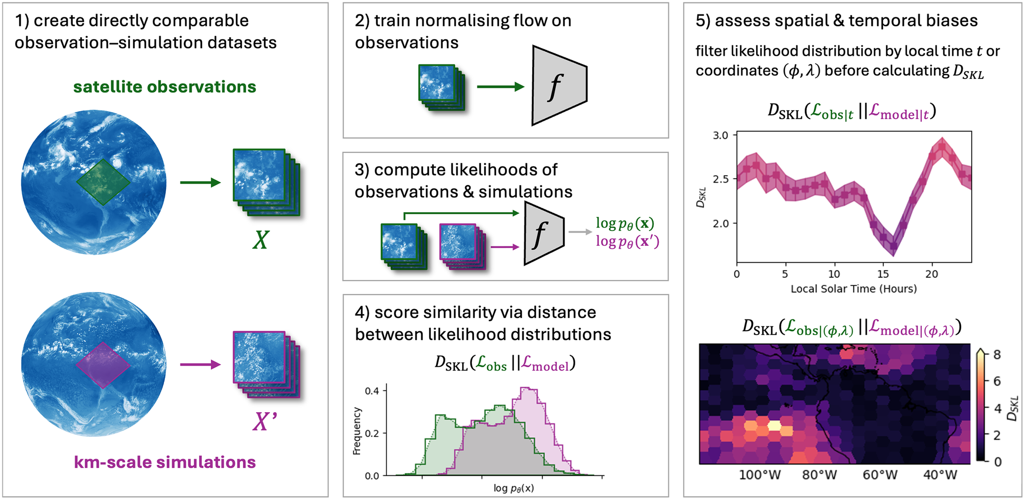
Figure 2. Long description
The flowchart is organized into five numbered panels.
* Panel 1: Create directly comparable observation-simulation datasets. It shows two globes. The top globe, labeled satellite observations in green, has a green square patch extracted into a stack labeled X. The bottom globe, labeled km-scale simulations in purple, has a purple square patch extracted into a stack labeled X prime.
* Panel 2: Train normalizing flow on observations. A green arrow points from a stack of green patches into a trapezoidal block labeled f.
* Panel 3: Compute likelihoods of observations and simulations. Green and purple patches point into the f block, which outputs log p theta (x) in green and log p theta (x prime) in purple.
* Panel 4: Score similarity via distance between likelihood distributions. A histogram shows two overlapping distributions of log p theta (x). The green distribution is shifted left, and the purple distribution is shifted right. The mathematical formula above is D sub S K L (L sub obs || L sub model).
* Panel 5: Assess spatial and temporal biases. This panel contains two graphs. The top graph is a line plot of D sub S K L versus Local Solar Time (Hours), showing a fluctuating trend with a sharp dip at 16 hours and a peak at 21 hours. The bottom graph is a geographical heat map of D sub S K L across South America and the Atlantic Ocean, with a color scale from 0 to 8, showing high values in the South Pacific and low values over the continent.
2.1. Preliminaries
A km-scale climate model, initialized at time
$ {t}_0 $
 , generates a trajectory of weather states
$ {\mathbf{x}}_1^{\prime },{\mathbf{x}}_2^{\prime },\dots $
, generates a trajectory of weather states
$ {\mathbf{x}}_1^{\prime },{\mathbf{x}}_2^{\prime },\dots $
 whose statistics define the simulated climate. Observations provide a corresponding sequence
$ {\mathbf{x}}_1,{\mathbf{x}}_2,\dots $
whose statistics define the simulated climate. Observations provide a corresponding sequence
$ {\mathbf{x}}_1,{\mathbf{x}}_2,\dots $
 representing the real climate system. Weather is intrinsically stochastic, so we cannot expect
$ {\mathbf{x}}_t={\mathbf{x}}_t^{\prime } $
representing the real climate system. Weather is intrinsically stochastic, so we cannot expect
$ {\mathbf{x}}_t={\mathbf{x}}_t^{\prime } $
 at any given time
$ t $
at any given time
$ t $
 . Instead, the task of climate model evaluation is to assess whether the statistics of the simulated climate are consistent with those of the observed system. Formally, we assume access to some observational dataset
$ \mathbf{X}=\left\{{\mathbf{x}}_1,\dots, {\mathbf{x}}_N\right\} $
. Instead, the task of climate model evaluation is to assess whether the statistics of the simulated climate are consistent with those of the observed system. Formally, we assume access to some observational dataset
$ \mathbf{X}=\left\{{\mathbf{x}}_1,\dots, {\mathbf{x}}_N\right\} $
 , generated from an unknown data-generating distribution,
$ {\mathbf{x}}_i\sim {p}_{\mathrm{obs}}\left(\mathbf{x}\right) $
, generated from an unknown data-generating distribution,
$ {\mathbf{x}}_i\sim {p}_{\mathrm{obs}}\left(\mathbf{x}\right) $
 , and a simulated dataset
$ {\mathbf{X}}^{\prime }=\left\{{\mathbf{x}}_1^{\prime },\dots, {\mathbf{x}}_M^{\prime}\right\} $
, and a simulated dataset
$ {\mathbf{X}}^{\prime }=\left\{{\mathbf{x}}_1^{\prime },\dots, {\mathbf{x}}_M^{\prime}\right\} $
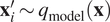
 drawn from a km-scale model distribution
$ {\mathbf{x}}_i^{\prime}\sim {q}_{\mathrm{model}}\left(\mathbf{x}\right) $
drawn from a km-scale model distribution
$ {\mathbf{x}}_i^{\prime}\sim {q}_{\mathrm{model}}\left(\mathbf{x}\right) $
 . Here, each sample
$ {\mathbf{x}}_i $
. Here, each sample
$ {\mathbf{x}}_i $
 (and
$ {\mathbf{x}}_i^{\prime } $
(and
$ {\mathbf{x}}_i^{\prime } $
 ) corresponds to a local patch rather than a global snapshot. Multiple models may be considered, each creating different datasets
$ {\mathbf{X}}_1^{\prime },{\mathbf{X}}_2^{\prime },\dots, {\mathbf{X}}_K^{\prime } $
) corresponds to a local patch rather than a global snapshot. Multiple models may be considered, each creating different datasets
$ {\mathbf{X}}_1^{\prime },{\mathbf{X}}_2^{\prime },\dots, {\mathbf{X}}_K^{\prime } $
 . The evaluation problem is to quantify the similarity between
$ {p}_{\mathrm{obs}} $
. The evaluation problem is to quantify the similarity between
$ {p}_{\mathrm{obs}} $
 and
$ {q}_{\mathrm{model},k} $
and
$ {q}_{\mathrm{model},k} $
 .
.
2.2. Creating directly comparable observation–simulation datasets
Evaluating climate models against observations requires directly comparable observation and simulation datasets that represent the same variable and lie on the same grid. For neural network applications, the grid should represent sub-regions of the globe as a contiguous matrix and provide an equal-area discretization of the sphere to ensure global statistical consistency.
2.2.1. Conservative remapping of geospatial data on curvilinear grids
We reproject all datasets onto the HEALPix grid (Górski et al., Reference Górski, Hivon, Banday, Wandelt, Hansen, Reinecke and Bartelmann2005), which satisfies the above-mentioned requirements. To minimize interpolation artefacts that could bias model–observation comparisons, we use a first-order conservative remapping scheme (Jones, Reference Jones1999). This requires constructing pixel boundaries for the satellite dataset from pixel (center) coordinates. We approximate each corner as the midpoint in latitude–longitude space between the four neighboring pixel centers on the curvilinear grid. At km-scale resolution, this approximation is sufficiently accurate as spherical distortions are negligible.
2.2.2. Removing large-scale biases via histogram matching
To evaluate small-scale features rather than large-scale biases, we standardize simulated data using histogram matching. Let
$ {F}_{\mathrm{obs}} $
 and
$ {F}_{\mathrm{sim}} $
and
$ {F}_{\mathrm{sim}} $
 denote the empirical cumulative distribution functions (CDFs) of observations and simulations, respectively, computed jointly across all spatial points. Each simulated value
$ {\mathbf{x}}^{\prime } $
denote the empirical cumulative distribution functions (CDFs) of observations and simulations, respectively, computed jointly across all spatial points. Each simulated value
$ {\mathbf{x}}^{\prime } $
 is transformed as
$ {\tilde{\mathbf{x}}}^{\prime }={F}_{\mathrm{obs}}^{-1}\left({F}_{\mathrm{sim}}\left({\mathbf{x}}^{\prime}\right)\right), $
is transformed as
$ {\tilde{\mathbf{x}}}^{\prime }={F}_{\mathrm{obs}}^{-1}\left({F}_{\mathrm{sim}}\left({\mathbf{x}}^{\prime}\right)\right), $
 so that the transformed simulation
$ {\tilde{\mathbf{x}}}^{\prime } $
so that the transformed simulation
$ {\tilde{\mathbf{x}}}^{\prime } $
 follows the observed distribution. In practice, the CDFs are constructed from discretized histograms, and the mapping is implemented by finding the smallest observation bin whose cumulative probability exceeds that of the simulated value.
2.3. Generative model likelihoods for similarity estimation
We fit a likelihood-based generative model
$ p\left(\mathbf{x};\theta \right) $
 to the observational dataset
$ \mathbf{X} $
to the observational dataset
$ \mathbf{X} $
 , with trainable parameters
$ \theta $
, with trainable parameters
$ \theta $
 . We use a normalizing flow (see Section 2.4), although any likelihood-based generative model could be used. Here, each
$ {\mathbf{x}}_i\in \mathbf{X} $
. We use a normalizing flow (see Section 2.4), although any likelihood-based generative model could be used. Here, each
$ {\mathbf{x}}_i\in \mathbf{X} $
 represents a square spatial patch of the input data on the HEALPix grid. The trained model provides a likelihood distribution for observational snapshots under
$ p\left(\mathbf{x};\theta \right) $
represents a square spatial patch of the input data on the HEALPix grid. The trained model provides a likelihood distribution for observational snapshots under
$ p\left(\mathbf{x};\theta \right) $
 against which model datasets are evaluated. Formally, we estimate discrete log likelihood distributions:

We then compute the symmetrized KL divergence between the two distributions of log likelihoods of the observed data,
$ {\mathrm{\mathcal{L}}}_{\mathrm{obs}} $
 , and the model data,
$ {\mathrm{\mathcal{L}}}_{\mathrm{model}} $
, and the model data,
$ {\mathrm{\mathcal{L}}}_{\mathrm{model}} $
 :
:

This divergence is zero if the two distributions are identical and increases without bound as they diverge, thus providing a metric quantifying the similarity between observations and simulations.
Likelihoods are computed for individual patches, which we can stratify by time or location to investigate temporal and spatial biases. Alongside each patch, we retain metadata: local solar time
$ t $
 and central latitude-longitude coordinates
$ \left(\phi, \lambda \right) $
and central latitude-longitude coordinates
$ \left(\phi, \lambda \right) $
 . To study temporal biases, we group by local solar time and compare the conditional likelihood distributions
$ {\mathrm{\mathcal{L}}}_{\mathrm{obs}\mid t} $
. To study temporal biases, we group by local solar time and compare the conditional likelihood distributions
$ {\mathrm{\mathcal{L}}}_{\mathrm{obs}\mid t} $
 and
$ {\mathrm{\mathcal{L}}}_{\mathrm{model}\mid t} $
and
$ {\mathrm{\mathcal{L}}}_{\mathrm{model}\mid t} $
 . To study spatial biases, we group by patch coordinates and compare
$ {\mathrm{\mathcal{L}}}_{\mathrm{obs}\mid \left(\phi, \lambda \right)} $
. To study spatial biases, we group by patch coordinates and compare
$ {\mathrm{\mathcal{L}}}_{\mathrm{obs}\mid \left(\phi, \lambda \right)} $
 and
$ {\mathrm{\mathcal{L}}}_{\mathrm{model}\mid \left(\phi, \lambda \right)} $
and
$ {\mathrm{\mathcal{L}}}_{\mathrm{model}\mid \left(\phi, \lambda \right)} $
 , computing
$ {D}_{\mathrm{SKL}} $
, computing
$ {D}_{\mathrm{SKL}} $
 within each subset.
2.4. Normalizing flow likelihoods
Normalizing flows are a family of generative models that use a sequence of invertible and differentiable transformations to map a simple base distribution (e.g., a standard normal) into a complex target distribution matching the data of interest (Dinh et al., Reference Dinh, Krueger and Bengio2015; Kingma and Dhariwal, Reference Kingma and Dhariwal2018). Unlike other generative models such as generative adversarial networks or variational autoencoders, which provide only implicit or approximate likelihoods, normalizing flows offer both tractable likelihood evaluation and efficient sampling.
Flow-based generative models define an expressive probability density on the data of interest
$ \mathbf{x}\in {\mathrm{\mathbb{R}}}^D $
 by applying an invertible, differentiable mapping
$ f\left(\cdot; \theta \right):{\mathrm{\mathbb{R}}}^D\to {\mathrm{\mathbb{R}}}^D $
by applying an invertible, differentiable mapping
$ f\left(\cdot; \theta \right):{\mathrm{\mathbb{R}}}^D\to {\mathrm{\mathbb{R}}}^D $
 to a simple base random variable
$ \mathbf{z} $
to a simple base random variable
$ \mathbf{z} $
 . Using the change-of-variables formula, the exact log likelihood of a given sample
$ \mathbf{x} $
. Using the change-of-variables formula, the exact log likelihood of a given sample
$ \mathbf{x} $
 is:
is:

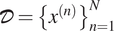
Given a training dataset
$ \mathcal{D}={\left\{{x}^{(n)}\right\}}_{n=1}^N $
 normalizing flows are trained to maximize the total log likelihood
$ {\sum}_n\log p\left({x}^{(n)};\theta \right) $
normalizing flows are trained to maximize the total log likelihood
$ {\sum}_n\log p\left({x}^{(n)};\theta \right) $
 with respect to
$ \theta $
with respect to
$ \theta $
 . We use a neural spline flow (NSF) (Durkan et al., Reference Durkan, Bekasov, Murray and Papamakarios2019), which employs monotonic rational quadratic splines to construct
$ f\left(\cdot; \theta \right) $
. We use a neural spline flow (NSF) (Durkan et al., Reference Durkan, Bekasov, Murray and Papamakarios2019), which employs monotonic rational quadratic splines to construct
$ f\left(\cdot; \theta \right) $
 (see Section 3.1 and Supplementary Appendix C).
3. Experiments and results
We use our framework for a case study evaluation of two km-scale models, IFS-FESOM and ICON against geostationary satellite observations from GOES-16. We analyze snapshots of top-of-atmosphere OLR and thereby focus our evaluation on deep convective clouds.
We use PyTorch lightning for neural network training and evaluation. We extend the NSF implementation provided by Durkan et al. (Reference Durkan, Bekasov, Murray and Papamakarios2019) to process our OLR datasets. We compare the results of our evaluation method to three baseline metrics: mean absolute error (MAE), multifractal parameters (Freischem et al., Reference Freischem, Weiss, Christensen and Stier2024), and spherical convolutional Wasserstein distance (SCWD, Garrett et al., Reference Garrett, Harris, Li and Wang2024).
3.1. Datasets and experimental setup
3.1.1. Kilometer-scale OLR simulations
We evaluate data from two global km-scale coupled models: ICON (Hohenegger et al., Reference Hohenegger, Korn, Linardakis, Redler, Schnur, Adamidis, Bao, Bastin, Behravesh, Bergemann, Biercamp, Bockelmann, Brokopf, Brüggemann, Casaroli, Chegini, Datseris, Esch, George, Giorgetta, Gutjahr, Haak, Hanke, Ilyina, Jahns, Jungclaus, Kern, Klocke, Kluft, Kölling, Kornblueh, Kosukhin, Kroll, Lee, Mauritsen, Mehlmann, Mieslinger, Naumann, Paccini, Peinado, Praturi, Putrasahan, Rast, Riddick, Roeber, Schmidt, Schulzweida, Schütte, Segura, Shevchenko, Singh, Specht, Stephan, von Storch, Vogel, Wengel, Winkler, Ziemen, Marotzke and Stevens2023) and IFS-FESOM (Rackow et al., Reference Rackow, Pedruzo-Bagazgoitia, Becker, Milinski, Sandu, Aguridan, Bechtold, Beyer, Bidlot, Boussetta, Deconinck, Diamantakis, Dueben, Dutra, Forbes, Ghosh, Goessling, Hadade, Hegewald, Jung, Keeley, Kluft, Koldunov, Koldunov, Kölling, Kousal, Kühnlein, Maciel, Mogensen, Quintino, Polichtchouk, Reuter, Sármány, Scholz, Sidorenko, Streffing, Sützl, Takasuka, Tietsche, Valentini, Vannière, Wedi, Zampieri and Ziemen2025). Both models parametrize radiation, turbulence, and cloud microphysics, but IFS includes more parametrizations such as deep and shallow convection. ICON directly outputs OLR (
$ {\mathrm{W}/\mathrm{m}}^2 $
 ) while IFS provides top net thermal radiation (ttr) equal to negative OLR accumulated over each hour (
$ {\mathrm{J}/\mathrm{m}}^2 $
) while IFS provides top net thermal radiation (ttr) equal to negative OLR accumulated over each hour (
$ {\mathrm{J}/\mathrm{m}}^2 $
 ), which we convert to OLR using:
$ \mathrm{OLR}=-\mathrm{ttr}/\left(3600\hskip0.24em \mathrm{s}\right) $
), which we convert to OLR using:
$ \mathrm{OLR}=-\mathrm{ttr}/\left(3600\hskip0.24em \mathrm{s}\right) $
 . We analyze nextGEMS cycle 4 simulations (Segura et al., Reference Segura, Pedruzo-Bagazgoitia, Weiss, Müller, Rackow, Lee, Dolores-Tesillos, Benedict, Aengenheyster, Aguridan, Arduini, Baker, Bao, Bastin, Baulenas, Becker, Beyer, Bockelmann, Brüggemann, Brunner, Cheedela, Das, Denissen, Dragaud, Dziekan, Ekblom, Engels, Esch, Forbes, Frauen, Freischem, García-Maroto, Geier, Gierz, González-Cervera, Grayson, Griffith, Gutjahr, Haak, Hadade, Haslehner, ul Hasson, Hegewald, Kluft, Koldunov, Koldunov, Kölling, Koseki, Kosukhin, Kousal, Kuma, Kumar, Li, Maury, Meindl, Milinski, Mogensen, Niraula, Nowak, Praturi, Proske, Putrasahan, Redler, Santuy, Sármány, Schnur, Scholz, Sidorenko, Spät, Sützl, Takasuka, Tompkins, Uribe, Valentini, Veerman, Voigt, Warnau, Wachsmann, Wacławczyk, Wedi, Wieners, Wille, Winkler, Wu, Ziemen, Zimmermann, Bender, Bojovic, Bony, Bordoni, Brehmer, Dengler, Dutra, Faye, Fischer, van Heerwaarden, Hohenegger, Järvinen, Jochum, Jung, Jungclaus, Keenlyside, Klocke, Konow, Klose, Malinowski, Martius, Mauritsen, Mellado, Mieslinger, Mohino, Pawłowska, Peters-von Gehlen, Sarré, Sobhani, Stier, Tuppi, Vidale, Sandu and Stevens2025), initialized with ERA5 reanalysis (Hersbach et al., Reference Hersbach, Bell, Berrisford, Hirahara, Horányi, Muñoz-Sabater, Nicolas, Peubey, Radu, Schepers, Simmons, Soci, Abdalla, Abellan, Balsamo, Bechtold, Biavati, Bidlot, Bonavita, De Chiara, Dahlgren, Dee, Diamantakis, Dragani, Flemming, Forbes, Fuentes, Geer, Haimberger, Healy, Hogan, Hólm, Janisková, Keeley, Laloyaux, Lopez, Lupu, Radnoti, de Rosnay, Rozum, Vamborg, Villaume and Thépaut2020) at 00:00 UTC on 20 January 2020 and integrated for 30 years at
$ \sim $
. We analyze nextGEMS cycle 4 simulations (Segura et al., Reference Segura, Pedruzo-Bagazgoitia, Weiss, Müller, Rackow, Lee, Dolores-Tesillos, Benedict, Aengenheyster, Aguridan, Arduini, Baker, Bao, Bastin, Baulenas, Becker, Beyer, Bockelmann, Brüggemann, Brunner, Cheedela, Das, Denissen, Dragaud, Dziekan, Ekblom, Engels, Esch, Forbes, Frauen, Freischem, García-Maroto, Geier, Gierz, González-Cervera, Grayson, Griffith, Gutjahr, Haak, Hadade, Haslehner, ul Hasson, Hegewald, Kluft, Koldunov, Koldunov, Kölling, Koseki, Kosukhin, Kousal, Kuma, Kumar, Li, Maury, Meindl, Milinski, Mogensen, Niraula, Nowak, Praturi, Proske, Putrasahan, Redler, Santuy, Sármány, Schnur, Scholz, Sidorenko, Spät, Sützl, Takasuka, Tompkins, Uribe, Valentini, Veerman, Voigt, Warnau, Wachsmann, Wacławczyk, Wedi, Wieners, Wille, Winkler, Wu, Ziemen, Zimmermann, Bender, Bojovic, Bony, Bordoni, Brehmer, Dengler, Dutra, Faye, Fischer, van Heerwaarden, Hohenegger, Järvinen, Jochum, Jung, Jungclaus, Keenlyside, Klocke, Konow, Klose, Malinowski, Martius, Mauritsen, Mellado, Mieslinger, Mohino, Pawłowska, Peters-von Gehlen, Sarré, Sobhani, Stier, Tuppi, Vidale, Sandu and Stevens2025), initialized with ERA5 reanalysis (Hersbach et al., Reference Hersbach, Bell, Berrisford, Hirahara, Horányi, Muñoz-Sabater, Nicolas, Peubey, Radu, Schepers, Simmons, Soci, Abdalla, Abellan, Balsamo, Bechtold, Biavati, Bidlot, Bonavita, De Chiara, Dahlgren, Dee, Diamantakis, Dragani, Flemming, Forbes, Fuentes, Geer, Haimberger, Healy, Hogan, Hólm, Janisková, Keeley, Laloyaux, Lopez, Lupu, Radnoti, de Rosnay, Rozum, Vamborg, Villaume and Thépaut2020) at 00:00 UTC on 20 January 2020 and integrated for 30 years at
$ \sim $
 10 km atmospheric and 5 km ocean resolution. Model outputs are saved on the HEALPix grid. We use the finest resolution available, HEALPix zoom level 9, with a grid spacing of
$ \sim 0.115{}^{\circ}\approx 12.7\ \mathrm{km} $
10 km atmospheric and 5 km ocean resolution. Model outputs are saved on the HEALPix grid. We use the finest resolution available, HEALPix zoom level 9, with a grid spacing of
$ \sim 0.115{}^{\circ}\approx 12.7\ \mathrm{km} $
 .
.
3.1.2. GOES-16 OLR observations
We use observations from the GOES-16 satellite, launched in 2016 and positioned at 75.2°W. It carries the Advanced Baseline Imager (ABI), which provides full-disk images at 2 km resolution every 10 minutes (Schmit and Gunshor, Reference Schmit, Gunshor, Goodman, Schmit, Daniels and Redmon2020). We estimate OLR from ABI narrowband infrared measurements (Supplementary Appendix A; Lee et al., Reference Lee, Laszlo and Gruber2010) and remap it onto the HEALPix grid using the climate data operators’ conservative remapping tool (Schulzweida, Reference Schulzweida2023).
3.1.3. Region, time period, and train/val/test split
We analyze the tropical band visible from GOES-16, which ranges from 20° to 130°W, using 1 year of data (2024) at hourly intervals. We split the dataset temporally into training, validation, and test sets for our machine-learning models. More specifically, we use days 1 to 15 of each month for training, days 20 to 23 for validation, and days 26 to 29 for testing. We leave gaps to reduce information leakage between the three datasets; this choice is motivated by the atmospheric predictability in the tropics, where small-scale (
$ < $
 100 km) features typically lose memory of their initial conditions within 5–7 days (Judt, Reference Judt2020).
3.1.4. Data processing
We empirically determine the range and distribution of values in our model and observation datasets from the training set by computing OLR histograms at a bin width of
$ 0.5{\ \mathrm{W}/\mathrm{m}}^2 $
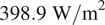
 . The histograms are used to derive the CDFs of our three datasets and create lookup tables between the model and observation CDFs for histogram matching of the simulated OLR data to GOES OLR observations. Finally, OLR values are scaled to the range (0, 1) using empirically determined GOES minimum (
$ 94.1{\ \mathrm{W}/\mathrm{m}}^2 $
. The histograms are used to derive the CDFs of our three datasets and create lookup tables between the model and observation CDFs for histogram matching of the simulated OLR data to GOES OLR observations. Finally, OLR values are scaled to the range (0, 1) using empirically determined GOES minimum (
$ 94.1{\ \mathrm{W}/\mathrm{m}}^2 $
 ) and maximum (
$ 398.9{\ \mathrm{W}/\mathrm{m}}^2 $
) and maximum (
$ 398.9{\ \mathrm{W}/\mathrm{m}}^2 $
 ) OLR values. All three datasets are patched into
$ 64\times 64 $
) OLR values. All three datasets are patched into
$ 64\times 64 $
 pixel patches with a 32-pixel stride. For GOES, this yields 1,127,251 training and 380,781 validation patches.
3.1.5. Training a NSF on GOES-16 observations
We train an NSF (Durkan et al., Reference Durkan, Bekasov, Murray and Papamakarios2019) to model the GOES-16 OLR data. The model was trained for 20 epochs on 1 NVIDIA A100 GPU with a batch size of 64. Trained in an unsupervised fashion to maximize dataset likelihood (Section 2.4), the model achieves average log likelihoods of 3.56 and 3.53 per pixel on the training and validation sets, respectively. Likelihoods are normalized per pixel to enable comparison across resolutions. The model assigns highest likelihoods to cloud-free patches and lowest likelihoods to patches containing popcorn convection; it generates realistic OLR patches, and sensitivity tests confirm robustness to NSF hyperparameters (Supplementary Appendix C).
3.2. Quantitative evaluation of km-scale models against observations
We evaluate the realism of OLR fields simulated by km-scale models by computing the symmetrized KL divergence of the likelihood distribution between each model output and the observations. Models that replicate the observed climate distribution in the input region will have a low
$ {D}_{\mathrm{SKL}} $
 (approaching 0), while models which fail to capture (high-resolution) features of the data distribution will have higher
$ {D}_{\mathrm{SKL}} $
(approaching 0), while models which fail to capture (high-resolution) features of the data distribution will have higher
$ {D}_{\mathrm{SKL}} $
 . We additionally calculate
$ {D}_{\mathrm{SKL}} $
. We additionally calculate
$ {D}_{\mathrm{SKL}} $
 between two halves of each dataset for comparison. All
$ {D}_{\mathrm{SKL}} $
between two halves of each dataset for comparison. All
$ {D}_{\mathrm{SKL}} $
 calculations in this section discretize likelihood distributions using 100 bins, and error bounds were estimated using bootstrap resampling.
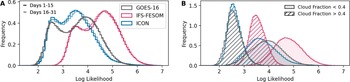
The likelihood distributions of both observations and simulations are bimodal (Figure 3). The two modes correspond to clear and cloudy scenes, with cloudy being defined as patches containing over 40% cloudy pixels based on a threshold of
$ 200{\ \mathrm{W}/\mathrm{m}}^2 $
 . Although the peaks of both modes are of similar sizes in GOES and ICON, the IFS-FESOM simulations seem to contain more clear sky than cloudy patches. The NSF assigns particularly high likelihoods to cloud-free scenes, whereas cloudy scenes with a lot of small-scale variability get assigned the lowest likelihoods (Supplementary Appendix Figure D3). The two models show distinct biases (Table 1). ICON is closer to observations and shows lower divergence over land than ocean, while IFS-FESOM diverges strongly. Notably, IFS-FESOM scores significantly worsen when the likelihood distribution is split by ocean and land.
$ {D}_{\mathrm{SKL}} $
. Although the peaks of both modes are of similar sizes in GOES and ICON, the IFS-FESOM simulations seem to contain more clear sky than cloudy patches. The NSF assigns particularly high likelihoods to cloud-free scenes, whereas cloudy scenes with a lot of small-scale variability get assigned the lowest likelihoods (Supplementary Appendix Figure D3). The two models show distinct biases (Table 1). ICON is closer to observations and shows lower divergence over land than ocean, while IFS-FESOM diverges strongly. Notably, IFS-FESOM scores significantly worsen when the likelihood distribution is split by ocean and land.
$ {D}_{\mathrm{SKL}} $
 between training and validation splits is very low for all datasets, confirming internal consistency (Supplementary Appendix Table D4).
Histograms of log likelihoods under the neural spline flow trained on GOES satellite data. (A) shows the likelihood distribution of GOES compared with two km-scale simulations IFS-FESOM and ICON. (B) shows likelihood distributions split by fraction of cloudy pixels per patch.
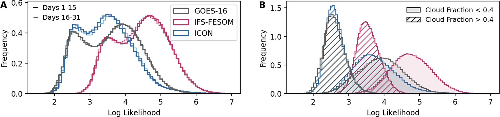
Figure 3. Long description
Two side-by-side histograms. Both share a y-axis labeled Frequency and an x-axis labeled Log Likelihood ranging from 0 to 7.
Panel A: Compares three datasets.
* G O E S-16 (grey) shows a bimodal distribution with peaks near 2.5 and 4.0.
* I C O N (blue) follows a similar bimodal shape but shifted slightly higher, with peaks near 2.6 and 3.8.
* I F S-F E S O M (magenta) shows a distinct distribution shifted further right, with a primary peak near 4.8.
* Solid lines represent Days 1-15 and dashed lines represent Days 16-31, showing high temporal consistency.
Panel B: Splits the same three datasets by cloud fraction.
* Solid filled areas represent Cloud Fraction less than 0.4. These distributions are shifted to the right, with peaks between 3.5 and 5.0.
* Hatched areas represent Cloud Fraction greater than 0.4. These distributions are shifted significantly to the left, with sharp peaks concentrated between 2.0 and 3.0.
* The grey G O E S-16 and blue I C O N distributions overlap heavily in the high cloud fraction zone, while the magenta I F S-F E S O M remains the furthest right in both categories.
Symmetrized KL divergence of likelihood distributions of outgoing longwave radiation fields of two km-scale models IFS-FESOM and ICON, compared to GOES-16 geostationary satellite observations

Table 1. Long description
The table consists of three columns of data under the headers Overall, Ocean, and Land.
* The first row displays the symmetrized K L divergence of the likelihood distribution of IFS-FESOM relative to G O E S. The values are 1.494 plus or minus 0.036 for Overall, 2.433 plus or minus 0.044 for Ocean, and 2.332 plus or minus 0.069 for Land.
* The second row displays the symmetrized K L divergence of the likelihood distribution of I C O N relative to G O E S. The values are 0.057 plus or minus 0.001 for Overall, 0.110 plus or minus 0.001 for Ocean, and 0.008 plus or minus 0.001 for Land.
3.3. Revealing spatial and temporal patterns of divergence
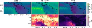
Next, we examine the spatial and temporal origins of the biases identified by our metric by conditioning likelihood distributions on patch center coordinates or local solar time (Section 2.3). This analysis reveals distinct spatial and temporal patterns in model errors. Figure 4 shows the divergence at each patch location. For ICON, the higher divergence over the ocean (Table 1) is concentrated in the south-western part of the domain, where deep convection is largely absent. By contrast, convectively active regions are represented exceptionally well. This indicates that ICON realistically captures deep convective structures but struggles in regimes dominated by shallow convection and clear-sky conditions. IFS-FESOM, by comparison, exhibits high divergence more uniformly across the domain, with larger errors in convectively active regions, pointing to systematic biases in both cloudy and clear-sky regimes.
Analysis of spatial biases in outgoing longwave radiation of two km-scale models, IFS-FESOM and ICON, compared to GOES-16 geostationary satellite observations. Top row: maps of mean log likelihood for each patch across the input region. Bottom row: maps of symmetrized KL divergence between patch-wise likelihood distributions of IFS-FESOM and ICON compared to GOES-16.
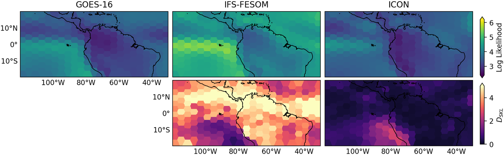
Figure 4. Long description
The figure consists of five panels arranged in two rows. All panels show a geographical region spanning 100 degrees West to 40 degrees West and 10 degrees South to 10 degrees North, centered on Central and South America.
Top Row: Three maps showing Log Likelihood on a color scale from 3 (dark purple) to 6 (yellow).
* Left: G O E S-16 shows moderate likelihood values with a dark purple core over the Amazon basin.
* Middle: I F S-F E S O M shows significantly higher likelihood values, particularly in a bright yellow horizontal band across the Pacific Ocean west of South America.
* Right: I C O N shows lower likelihood values overall, with deep purple concentrated along the South American coast and the Atlantic.
Bottom Row: Two maps showing Symmetrized K L Divergence (D sub S K L) on a scale from 0 (dark purple) to 5 (pale yellow).
* Middle: I F S-F E S O M compared to G O E S-16 shows high divergence (yellow/orange) across the northern half of the map and the Amazon, with lower divergence (purple) in the Southwest Pacific.
* Right: I C O N compared to G O E S-16 shows much lower divergence overall, appearing mostly dark purple, with a slight increase to pink/purple in the Southwest Pacific region.
Vertical color bars on the right side of each row define the numerical scales for Log Likelihood (top) and D sub S K L (bottom).
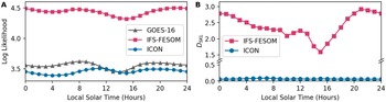
Temporal stratification reveals further structure in model biases (Figure 5). Deep convective clouds respond strongly to the diurnal cycle of incoming solar radiation, especially over land (Jones et al., Reference Jones, Stengel and Stier2023). Since clouds modulate OLR, their diurnal cycle is also expressed in the OLR signal. Climate models are known to struggle to capture the diurnal cycle accurately (Yin and Porporato, Reference Yin and Porporato2017), making it a critical test of model realism. The divergence between IFS-FESOM and GOES observations shows clear time-of-day dependence, with agreement improving in the early afternoon when convective activity peaks. While snapshot-based evaluation allows temporal analysis of biases, likelihood histograms converge after about 1 month (Supplementary Appendix Figure D5).
Analysis of temporal biases of two km-scale climate models, ICON and IFS-FESOM, compared to GOES-16 geostationary satellite observations. Diurnal cycle of (A) average log likelihood and (B) the divergence between likelihood distributions of models and observations.
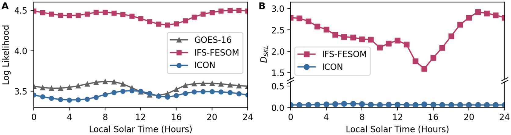
Figure 5. Long description
A two-panel line graph. Both panels share an x-axis labeled Local Solar Time in Hours, ranging from 0 to 24.
Panel A, titled Log Likelihood on the y-axis (range 3.3 to 4.5), shows three data series:
* I F S-F E S O M (magenta squares) maintains the highest values, fluctuating between 4.3 and 4.5 with a slight dip around 14 hours.
* G O E S-16 (gray triangles) follows a lower, stable path between 3.4 and 3.6.
* I C O N (blue circles) tracks closely below G O E S-16, ranging from 3.4 to 3.5.
Panel B, titled D sub S K L on the y-axis, features a broken axis with a lower section from 0.0 to 0.5 and an upper section from 1.5 to 3.0. It shows two data series:
* I F S-F E S O M (magenta squares) starts high at 2.8, gradually declines to a minimum of 1.6 at 15 hours, then rises sharply back to 2.9 by 21 hours.
* I C O N (blue circles) remains nearly flat and constant near the 0.1 mark across the entire 24-hour period.
3.4. Metric comparison and sensitivity tests
We compare our method to relevant baselines: OLR MAE, SCWD, and multifractal parameters (Supplementary Appendix D). MAE reveals opposite biases to our approach, reflecting large-scale mean errors that are removed by histogram matching. SCWD closely mirrors MAE, indicating sensitivity to similar large-scale discrepancies. In contrast, multifractal analysis finds biases more similar to those revealed by our likelihood-based approach, consistent with both approaches probing fine-scale spatial variability. Our method is, however, more expressive, capturing model errors beyond scaling behavior alone. We further assess the sensitivity of our results to variations in NSF architecture, data standardization, and input patch size. Likelihood scores are consistent with those obtained for the original model setup. This robustness emphasizes the ability of our method to reliably evaluate models based on small-scale structural features.
4. Discussion
Climate model evaluation is critical for ensuring that simulations faithfully represent the Earth system and provide reliable climate projections. Traditional evaluation methods, developed for low-resolution models, rely on bias metrics or low-order statistics and therefore cannot assess the spatial and temporal structures explicitly resolved at kilometer scale. To address this gap, we introduce a new framework that derives a quantitative similarity metric from the likelihood distribution learned by a normalizing flow model. Unlike existing metrics, this approach directly measures the similarity of distributions of simulated and observed snapshots. To facilitate the direct, fine-scale focused comparison between models and observations, we present a dataset-agnostic procedure for homogenizing dataset grid projections and removing large-scale biases via histogram matching.
We present a case study evaluation of two km-scale climate models, IFS-FESOM and ICON. Our results demonstrate that the likelihood-based method can robustly distinguish between models and observations, identifying spatio-temporally local biases in both models. Overall, ICON exhibits closer agreement with observations across regions and the diurnal cycle than IFS-FESOM. Nonetheless, it has a slight shift toward lower likelihoods compared with GOES, most likely because it simulates too small, unorganized convective cells, as expected for km-scale models with no convective parameterization (Wille et al., Reference Wille, Koch, Becker and Fischer2025; Takasuka et al., Reference Takasuka, Becker and Bao2026). IFS-FESOM has an opposite consistent bias toward higher likelihoods, due to more organized convection and thus larger structures and clearer sky regions in OLR fields.
Our likelihood-based approach provides an objective, quantitative, and dataset-agnostic metric that captures both overall similarity and the spatial–temporal structure of model biases. The comparison with MAE and SCWD highlights that our framework provides a complementary perspective. While MAE and SCWD capture magnitude biases locally and in regional distributions, our method directly probes fine-scale spatial structures in simulated fields, offering sensitivity to physical processes such as cloud formation at resolutions relevant for km-scale models. For a comprehensive evaluation of model biases, traditional metrics need to be used alongside fine-scale focused methods such as the likelihood-based evaluation introduced here. Histogram matching removes differences in the OLR distribution, thereby discarding information about absolute magnitude biases. This choice is intentional to isolate morphological differences between models and observations. Alternative normalization strategies could be adopted if the evaluation objective is to retain sensitivity to absolute biases.
The framework introduced here enables rigorous comparison of simulations with observations, offering guidance for the calibration and improvement of next-generation kilometer-scale climate models. While our case study focused on outgoing longwave radiation, the framework is readily extensible. Future work includes incorporating additional variables, such as shortwave radiation, water vapor, or precipitation for a more comprehensive assessment of model realism.
Supplementary material
The supplementary material for this article can be found at http://doi.org/10.1017/eds.2026.10054.
Acknowledgements
This work used supercomputing resources of the German Climate Computing Center (Deutsches Klimarechenzentrum, DKRZ) granted by its Scientific Steering Committee (WLA) under project ID 1153. We would also like to thank the anonymous reviewers for their constructive comments, who helped improve this manuscript.
Author contribution
Conceptualization: L.J.F., T.R., R.C., P.S., H.M.C. Methodology: L.J.F., T.R., R.C., P.S., H.M.C. Data curation: L.J.F. Data visualization: L.J.F. Writing original draft: L.J.F. All authors approved the final submitted draft.
Competing interests
The authors declare no competing interests.
Data availability statement
NextGEMS production simulations for ICON and IFS-FESOM are archived by the German Climate Computing Center (DKRZ) and can be accessed via DKRZ’s supercomputer Levante after registration at https://luv.dkrz.de/register/. GOES-16 OLR data were derived from Level 1b radiance measurements, which were supplied by the National Oceanic and Atmospheric Administration (NOAA) and can be downloaded at https://console.cloud.google.com/marketplace/product/noaa-public/goes. Model training and likelihood estimation code can be found on GitHub: https://github.com/lillif/likelihoods-km-scale-models. The repository has also been archived on Zenodo at DOI: 10.5281/zenodo.19358989.
Ethical statement
The research meets all ethical guidelines, including adherence to the legal requirements of the study country.
Funding statement
L.J.F. acknowledges funding from the NERC Doctoral Training Partnership in Environmental Research Grant NE/S007474/1. H.M.C. was funded through the EERIE project (Grant Agreement No 101081383) funded by the European Union. University of Oxford’s contribution to EERIE is funded by UK Research and Innovation (UKRI) under the UK government’s Horizon Europe funding guarantee (grant number 10049639). H.M.C. was also funded through a Leverhulme Trust Research Leadership Award “Seamless Uncertainty Quantification for Earth System prediction” (SUQCES). P.S. and T.R. acknowledge funding from the EU’s Horizon Europe project Embed2Scale under grant agreement number 10113184. University of Oxford’s contribution to Embed2Scale is funded by UK Research and Innovation (UKRI) under the UK government’s Horizon Europe funding guarantee (grant number 10113603). P.S. also acknowledges funding from the European Union’s Horizon Europe project CleanCloud with grant agreement 101137639 University of Oxford’s contribution to CleanCloud is funded by UK Research and Innovation (UKRI) under the UK government’s Horizon Europe funding guarantee (grant number 10113611). T.R. also acknowledges funding from ARIA and DSIT and Pillar VC under the Encode: AI for Science Fellowship. Views and opinions expressed are however those of the author(s) only and do not necessarily reflect those of the European Union or the European Climate Infrastructure and Environment Executive Agency (CINEA). Neither the European Union nor the granting authority can be held responsible for them. For the purpose of Open Access, the author has applied a CC BY public copyright license to any Author Accepted Manuscript version arising from this submission.
Provenance statement
This article is part of the Climate Informatics 2026 proceedings and was accepted in Environmental Data Science on the basis of the Climate Informatics peer review process.



 Open access

